Appendix
Quantifying Real Estate Uncertainty: Let’s Think about the Inputs for Real Estate Simulation Models
In this Appendix, we want to tell you how we arrive at the real estate market price dynamics that we use, and how we simulate future real estate pricing to represent uncertainty, as realistically as we can.
In Chapter 7, we described how we use pricing factors to simulate future scenarios in the real estate market based on dynamics and probability functions that we input into the spreadsheet. We described a very basic and widely used dynamic pricing process known as the random walk. We described how private real estate markets include a random walk element but also include some other features: inertia (autoregression), cyclicality, and mean‐reversion.
In this Appendix, we want to take you a little deeper into the details, the nuts and bolts of our thinking and method for coming up with these important inputs. We want to give you some feeling for how this aspect of simulation analysis is part science and part art. We use a lot of judgment based on common sense (we think). But we also use some interesting empirical evidence and some relevant economic theory.
The “journey” in this Appendix isn’t for everybody. If you don’t want to get a little technical, and indeed if you don’t want to see “how the sausage is made,” then this Appendix may not be for you. We delve into some statistics and economic theory. But, to begin, we want to simply step back and think about the big picture of what we are trying to simulate. Real estate markets are embedded within what we call “the real estate system.”
A.1 The Real Estate System
Figure A.1 depicts the real estate system. There are three main elements: the space market, the asset market, and the development industry. The space market trades the rights to occupy and use built space, with landlords on the supply side and tenants on the demand side. Prevailing rental prices and occupancy rates characterize the equilibrium in the space market, and determine the net cash flows that are the fundamental benefit flows accruing to the owners of the property assets (landlords).
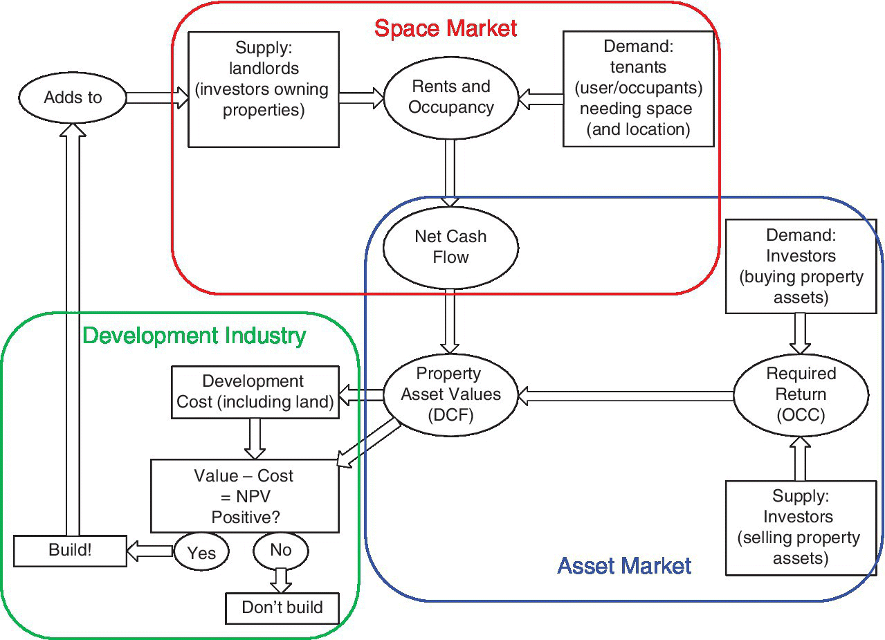
Figure A.1 The real estate system.
The asset market trades the long‐term ownership rights of the properties, with investors and owner‐occupiers buying and selling the assets. As a shortcut, we can represent the equilibrium price in the property asset market by the prevailing “cap rate,” or income yield rate. For example, if a property currently producing $100 per year net income would sell for $1000, then that pricing would be represented by a 10% cap rate. If the prevailing cap rate in the asset market falls to 9%, this would indicate that the price of such a property has risen to $1111 ($100/0.09).
The development industry is where and how financial capital builds physical capital, producing new buildings in the system, replacing older structures, or adding to the overall supply of built space in the space market. The development industry performs a basic calculation. It compares the present value of the expected benefit from a development project to the present value of the expected cost, including the land cost. As described in Chapters 2 and 11, if the computed NPV is positive, development is economical and generally proceeds.
The real estate system is dynamic. It is constantly changing, evolving over time. Exogenous growth and shocks in the economy affect demand for space. Financial capital flows into and out of the asset market and the development industry. When demand for space increases, rents and occupancies tend to rise, raising revenues from built properties. Other things being equal, this will raise property values, and this in turn will tend to stimulate new development—although development can be mitigated by possible rises in land costs. New development may put downward pressure on rents or result in increased vacancy in the space market, and this will reverse the preceding trend. Beliefs, behaviors, and actions in any element of the system will tend to affect the other elements of the system, at least after some time. The system tends toward a long‐run equilibrium, but often in fits and starts, and with a tendency to cycle around a long‐run trend. Decision‐makers in the system—especially investors and developers, and their financiers—try (or should try) to be forward‐looking, to forecast what the future of the relevant market is going to be. But no one has a crystal ball, and the future is almost never exactly as was predicted. Uncertainty in real estate markets and the dynamics of real estate pricing arise through and within all three elements of the system and in the interactions among them.
A.2 Sources of Uncertainty and Some Practical Advice for Simulation
Uncertainty about the future relevant for a real estate investment or project arises not only from within the real estate system, as described in the preceding text, but perhaps even more so, or more fundamentally, from outside the system. The underlying economy and sociopolitical and financial systems in which real estate markets are embedded provide a constant source of change.
Figure A.2 shows one visualization of this, together with a key point of practical advice. First, notice how many phenomena and considerations can influence the real estate system. Many (perhaps most) of these sources of uncertainty are exogenous to the real estate system itself. Figure A.2 lists 11 such causal factors—effectively, sources of uncertainty about the future. And this list is no doubt only partial. All of these are important phenomena that can substantially change the value of a given location or building for better or worse. We noted in Chapter 5 how difficult it is in practice to forecast accurately even one underlying determinative factor that can be a source of uncertainty (see Figure 5.2 in Box 5.2).
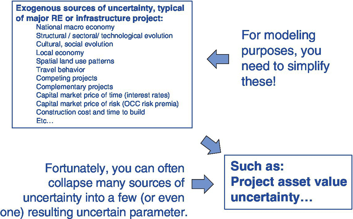
Figure A.2 Simplifying uncertainty for simulation modeling.
But Figure A.2 suggests a crucial point for simulation modeling. We can often collapse all of the sources of uncertainty into a single factor that captures the combined effect of everything regarding the determination of the value of the investment or project we are analyzing. For example, what ultimately matters from an investment perspective is generally the future value of the asset being built or invested in. Rather than attempting to model all of the possible determinants of this value in a causal structural model, we content ourselves with modeling the kind of dynamics and randomness that appear in historical empirical data about property price evolution. Such data reflects the combined effects of all the determinants of property values, and such values are likely a sufficient metric of investment performance.
This does not mean that analysts should not consider, or indeed study and seek to understand, the underlying causal elements that affect prices and values. Univariate modeling purely reflecting longitudinal time‐series behavior is no substitute for a deep understanding of the dynamic causal structure in the system. But an ever‐present challenge in effective, practical simulation analysis is to avoid excessive complexity. We must not “get lost in the weeds,” and we must not “lose sight of the forest for the trees blocking the view!”
There is no small degree of “art” in this process. An extensive knowledge of historical evidence and economic theory, combined with practical experience in the property markets and a good dose of common sense, are the ingredients behind the art of trimming down the model. The key point is to keep your eye on what will most directly and sensitively affect the output that is most important in the analysis. For real estate investments, this is typically the value of the property asset.
A simple example of this point occurs first in Chapter 9, where we demonstrated the application of simulation analysis to an existing, income‐producing property. To generate a future scenario, we applied a single series of pricing factor realizations to all elements of the operating net cash flow of the property. We did not try to generate separate factors to represent different realizations of uncertainty for rents, occupancy, operating expenses, capital improvement expenditures, and so forth. Of course, in the real world, all of these components of the net cash flow “dance to the beat of their own drums” to some extent. But, within the big picture of what matters for the overall investment performance, that does not matter, provided we can capture the combined effect of everything in a single pricing factor that we apply to the overall bottom line (or equally to all elements in an additive combination).
For example, if revenue equals price times quantity, and revenue is what we care about, then we can fully represent the uncertainty that matters either purely with a pricing factor applied to price, or purely with a quantity factor applied to quantity, or some combination of both that requires both pricing and quantity factors. We usually gain little by trying to be more complicated. And it is usually easiest to collapse all the important considerations onto a pricing factor. If the outcome is revenue increasing by 10%, then it does not matter if we simulate that as quantity increasing 10% with constant pricing, or price increasing 10% with constant quantity, or quantity and price each increasing 4.9% (1.049 × 1.049 = 1.10), or price increasing 3% with quantity increasing 6.8% (1.03 × 1.068 = 1.10), or whatever. Generally, the simplest and most elegant approach is to reflect everything in the pricing factor. (Of course, there will be exceptions. Always apply common sense.)
A.3 The Nature of Real Estate Price Dynamics and Uncertainty
Now let us consider the nature of real estate market price dynamics. This also encompasses the question of the magnitude of uncertainty or risk in the future pricing that might be relevant for a given property or project (see Box A.1 for some relevant concepts).
For this purpose, we can identify eight separate sources or components governing real estate price dynamics—that is, how prices change over time. These eight components combine in the real world to govern and characterize real estate price evolution. This evolution defines the nature and magnitude of risk or uncertainty that investors face. The eight components are:
- Long‐term trend rate;
- Volatility;
- Cyclicality;
- Mean‐reversion;
- Inertia (autoregression);
- Price dispersion (noise);
- Idiosyncratic drift;
- Black swans.
A description of each of these components is given in the following text, together with some discussion about their theoretical basis and quantitative nature or magnitude for the purpose of simulation modeling.
(1) Long‐term trend rate. The first source of uncertainty is the long‐term trend rate. That is, what is the secular rate of change that real estate prices tend to exhibit on average over the long run? (The term “secular” here refers to a long‐run trend that persists over time.) This rate is best considered in real terms—that is, net of monetary inflation. This trend component of real estate price dynamics is illustrated in Figure A.3, which shows almost a half‐century of history of an aggregate index of commercial property prices in the United States. The property price index is shown in nominal terms, but the consumer price index (CPI), which tracks cumulative inflation, is also shown in Figure A.3. The real change in property prices is the relative difference between the two lines over time. The property price index reflects “same property” price change—that is, the price change experienced by existing built properties, the type of price change that is experienced by investors.

Figure A.3 Commercial property prices, United States, 1969–2016: long‐term trend.
*Source: BLS, Moody’s/REAL, Moody’s/RCA, TBI, Author’s estimates.
The long‐term trend is evidenced by the difference in the value of the index at the end of the history as compared to the beginning, adjusting for temporary or cyclical effects. Over the entire 1969–2016 history, the nominal average rate of property price change was 3.8% per annum (measured by the geometric mean). But, over the same period, inflation averaged 4.0% per annum. If we measure trough‐to‐trough (1975–2009), the rates are 3.1% for property and 4.1% for inflation. Peak‐to‐peak (1972–2007), the rates are 4.1% and 4.7%, respectively. Thus, in real terms, property values have tended to decline slightly, growing less than inflation by typically less than 1% per year. This is in spite of the fact that property owners spend money on maintenance and upkeep of the properties. As the buildings on properties age, the property value reflects the depreciation of those built structures. Depreciation generally cannot be fully offset by spending on capital improvements. Thus, it is not surprising that the long‐term real price trend rate is slightly negative. However, this depends substantially on the role of land value over time. In places and times where land is very expensive and therefore makes up a large share of property value, the secular trend in property pricing might be more positive in real terms. This would be true if land values tend to grow in real terms, for land does not generally depreciate like built structures do.
Figure A.3 reflects the US national average, where, for properties with average‐age buildings, the land value fraction is typically only about half of the total property value. In denser, more land‐constrained countries (or in such places within the United States), the secular trend rate might be more positive. But it could be less positive in times and places of low or declining land value. Because we cannot know exactly the future secular trend in property values, this is a source of uncertainty in real estate prices. In most places, it probably ranges between, say, +1% and −2% in real terms (net of inflation).
(2) Volatility. This term was defined in Chapter 7 (see Box 7.2). There, we noted that “volatility” refers to the way prices change randomly, unpredictably from one period to the next. Volatility reflects the arrival of news—that is, unpredicted information that is relevant to the value of property. The price movements in each period relative to the prior values (akin to “capital returns,” the percentage changes in asset value) are also known as “innovations.” Volatility is clearly visible in the long‐term aggregate price index shown previously. Figure A.4 repeats that same index, highlighting some clear visual evidence of volatility. It shows up as random movements up and down in the price index.

Figure A.4 Commercial property prices, United States, 1969–2016: volatility.
Source: Moody’s/REAL, Moody’s/RCA, TBI, Author’s estimates.
The key feature of volatility is that it accumulates over time in the price levels. Volatility is the essential feature of the random walk component of asset price dynamics. As noted in Chapter 7, the random walk is “memoryless.” If news arrives that is positive, causing prices to rise (positive return in that period), then that holds no implication that prices will either continue rising in the next period or that they would tend to fall back in the next period. Thus, a random bump up in one period is “baked into” the price level as of the end of that period. Any change in the future will start from that new price level which reflects the “bump” from the previous news. In this sense, volatility “accumulates” over time in the price levels. Because the specific price innovations are not predictable in advance, volatility reflects risk, or a source of uncertainty for investors.
The historical empirical evidence in the United States, as indicated in Figure A.4 and numerous other similar indices, suggests that market volatility for commercial property may typically be around 10–15% per annum. This compares, for example, with the stock market, which generally exhibits annual volatility closer to 20%. But volatility varies over time and across different property space markets. Real estate price volatility also depends on the frequency at which it is computed, for example, monthly, quarterly, annually, biennially, etc. Because of inertia and cyclicality, real estate volatility measured on an equivalent annual basis is typically greater when measured at lower frequencies (longer “holding periods” in the periodic returns). For example, quarterly volatility might be 5%, while annual volatility is 10% and biennial volatility is 15%, all measured at a per‐annum rate.
(3) Cyclicality. The next component of real estate price dynamics is rather famous. It is the tendency of property markets to exhibit long‐term cycles, upswings followed by downswings or even “crashes.” Such cycles are prominent in the long‐term index that we have been looking at, which is repeated again in Figure A.5, delineating the long‐run historical cycles in the US commercial property market over the past half‐century. At least two complete cycles are evident, peak‐to‐peak, and trough‐to‐trough. Including the fractional cycles at either end of the depicted history, there are roughly three cycles during the almost half‐century covered. The average cycle period is 15–20 years. The index in Figure A.5 suggests that the down‐cycles can at least temporarily drop property asset prices by 30–40% on average, more in some markets.

Figure A.5 Commercial property prices, United States, 1969–2016: cyclicality and mean reversion.
Source: Moody’s/REAL, Moody’s/RCA, TBI, Author’s estimates.
The cycle in the asset market may, or may not, be echoed in the space market. The up‐cycle is sometimes characterized by over‐building and a rental market “bubble” (such as the late 1980s), but, other times, the cycle is more confined to the asset market (such as the mid‐2000s). Sometimes the down‐cycle is associated with a general economic recession (such as the global financial crisis of 2008–2009). Other times, there is little or no causal connection between the commercial property market and the wider macro‐economy (such as the late 1980s). There is some evidence that the property market cycle is related to behavior in the debt market—that is, the relative availability of debt capital for real estate investment. As noted earlier, the flow of financial capital (money) into and out of the real estate market can certainly move asset prices.
Although the tendency of real estate markets to cycle is well known, it is much more difficult to reliably predict the exact nature, timing, and magnitude of the cycles—and, most importantly, the “next downturn.” For this reason, cyclicality is an important source of uncertainty and risk for property investors and developers.
(4) Mean‐reversion. A component of real estate price dynamics that is closely related to cyclicality is the tendency toward mean‐reversion. Put simply, mean‐reversion is like gravity; it implies that “what goes up, must come down.” But, it is symmetrical: “what goes down must come back up too.” The idea is that if prices get too far out of line from the long‐run trend, they will tend to “correct” or “revert” back toward that long‐run trend.
What would cause prices to move far from the long‐run trend? It could be a tendency toward herd behavior in capital flows; or, it could be simply an exogenous streak of abnormally good, or bad, news.
What would cause prices to tend to revert toward the long‐run trend? It could be powerful economic fundamentals. Real estate assets consist of two components of value: the structure and the land. Structures are produced goods—in some sense, not unlike automobiles or refrigerators. There is substantial price elasticity of supply. The price (value) of structures cannot move very far from marginal production costs, or supply will respond (positively to price increases, negatively to price decreases), putting competitive pressures to keep structure prices near production costs. And, over the long run, structure production costs tend to keep pace with general inflation over time (roughly constant in real terms).
On the other hand, land is neither produced nor consumed, and is much more fixed in its supply. The land component of property value could evolve more like a random walk, without such tendency to revert toward a mean. So, the mean‐reversion tendency in real estate is rather weak and unreliable. This makes real estate price evolution more difficult to predict, and more uncertain than that of cars or refrigerators, for example.
Mean‐reversion may be stronger at the individual property level (tending to keep individual property values from moving too far from the local market average) than it is at the level of aggregate or market indices. Competitive pressures tend to drive mean‐reversion. Astute traders try to buy “bargains” (whose prices are far below average) and sell “winners” (whose prices are far above average). This acts to keep prices somewhat within bounds.
(5) Inertia (autoregression). This refers to the tendency of the price changes (capital returns) in one period to partially echo the price changes in the previous period. Technically, this process is known as “autoregression,” where the return in period t includes a fraction of the return in period t−1. The result is that, when prices start moving in one direction, they have a tendency to continue moving in that direction, to some extent, for a while.
What could cause such inertia in real estate prices? Inertia reflects the fact that property asset markets are not perfectly informationally efficient. This causes prices to be a bit sluggish or “sticky.” When news arrives that is relevant to asset value, it takes a while for that news to get fully reflected in transaction prices. This is because private real estate markets trade unique, whole assets. One cannot simply observe the change in prices at which other assets are trading and apply that change to a private real estate transaction. Each transaction is, essentially, a negotiation between two parties, neither of who knows for sure what the “market value” is of the unique asset they are trading.
Autoregression is similar to, and related to, both cyclicality and mean‐reversion. Indeed, autoregression partially overlaps with and reflects those other two phenomena. The difference is that autoregression can act either to push prices toward a long‐run mean, or away from it. Autoregression simply carries forward an (attenuated) “echo” of the previous period’s price change into the current period’s price change. This is depicted visually in Figure A.6.

Figure A.6 Commercial property prices, United States, 1969–2016: Inertia (autoregression).
Source: Moody’s/RCA, TBI, Author’s estimates.
True transaction price–based real estate index returns are only mildly autoregressive in the United States. Real estate markets aren’t too inefficient. Empirical evidence suggests that a typical annual frequency autoregressive parameter might be on the order of +0.1 to +0.3. In other words, the return in period t might include somewhere between one‐tenth and one‐third of the return in period t−1. (Price indices based on repeated appraisals of the same properties often show much greater autoregression, but this is partly due to the “anchoring” tendency in repeat‐appraisals, as the appraisers base their current opinion partly on their previous opinion.)
(6) Price dispersion (noise). The preceding phenomena and components of real estate price dynamics are systematic across all or most individual assets. Therefore, they occur at the aggregate level, and are evident in indices of markets or sub‐markets. But, now we want to introduce two phenomena that occur explicitly at the disaggregate level of individual properties, but that are not systematic and therefore do not appear in aggregate indices. The first is random price dispersion, also known as “noise.” As we have previously noted, no one knows for sure the exact market value of any property as of any point in time. Transaction prices are negotiated between two parties who both lack such knowledge. The result is that transaction prices are randomly dispersed around the true market values. In fact, the main practical definition of “market value” is that it is the mean of the distribution of possible actual transaction prices. Price dispersion causes an extra source of randomness in realized prices. Prior to any transaction, such noise is a source of uncertainty surrounding the future performance of the property as an investment.
The magnitude of price noise can be quantified in the standard deviation of transaction prices around previously predicted or estimated valuations. It can also be seen in the estimated intercept of regressions of squared residuals onto the time between sales in repeat‐sales regressions. Such empirical data in the United States and United Kingdom indicate dispersion standard deviations in the neighborhood of 10–15%, similar in magnitude to price index volatility. But the difference between noise and volatility is that, while volatility accumulates over time, noise does not. Noise happens only when, and if, a property is transacted. In essence, no matter how long the durations between transactions of a property, the magnitude of the noise surrounding its sale price remains approximately the same. In simulations, we model noise as a random “error” around the simulated “true” price level, whereas we model volatility as random deviations in the true returns (price increments).
(7) Idiosyncratic drift. The second component of real estate price dynamics that operates at the individual property level and not at the aggregate systematic level is what is called “idiosyncratic drift.” This is like volatility—random innovations that accumulate over time—except that idiosyncratic drift occurs only at the individual property level, uncorrelated with the market volatility. Idiosyncratic drift is depicted in Figure A.7, which shows how individual property price paths evolve separate from and independent of the market value index. For example, the market may be moving up in response to generally strong demand for space, but your particular building may have just lost its major tenant (who decided to move, perhaps, to a newer building). Your property’s value just fell, even though the market as a whole went up.
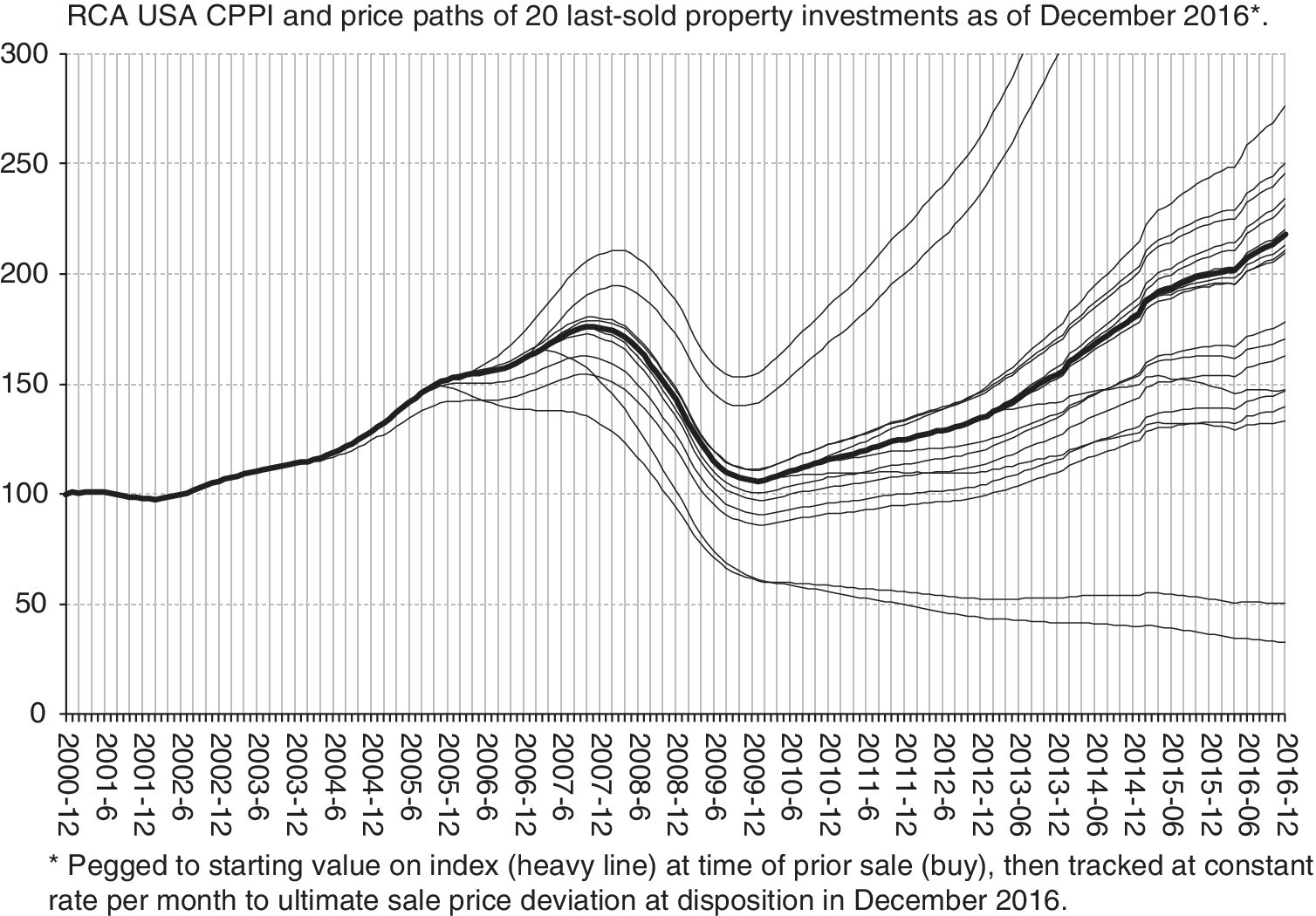
Figure A.7 Price paths of 20 property investments as of December 2016: idiosyncratic drift.
Empirical evidence from US commercial property price indices and the individual property transaction price residuals around such indices suggest that idiosyncratic drift is approximately equal in magnitude to market volatility, typically between 10% and 15% per annum, modeled as a random walk around the market index.
(8) Black swans. The last of the eight components of real estate price dynamics and uncertainty that we will identify applies once again at the aggregate level, systematically to all or most individual assets at a time. There are various words for this last type of phenomenon, including “fat tail events,” Bernoulli events, Poisson Arrivals, and others. The idea is that, on rare and unpredictable occasions, an event seems to come out of nowhere and have a huge, usually negative, effect on almost all assets. A famous such event was the global financial crisis of 2008–2009. During such an event, it is said that “covariance goes to one”—meaning that there is such contagion or mass panic that almost all assets fall together. A vivid illustration of this is shown in Figure A.8. The figure shows the relative price paths of all publicly traded commercial property investment companies (known as “real estate investment trusts”) monthly from 2000 through 2010, indexed to a starting value of 1.00. The price paths resemble random walks, with continuously accumulating volatility, until the financial crisis hits in 2008. Then, virtually all of the individual stocks collapse together. Black swans differ from normal volatility, in that they strike only rarely and usually bring unexpected losses rather than gains. Their effects also may not be as permanent as normal random walk–type volatility.

Figure A.8 Effect of the global financial crisis on price paths of all US real estate investment trusts: Black swan event (Financial Crisis, October 2008–March 2009).
Source: Authors.
A.4 Putting It All Together
The preceding section has introduced you to the eight major components of typical real estate market price dynamics. We have also noted some empirical evidence, as well as theoretical considerations, that help us to quantify and understand the causes and nature of these components.
In our simulation modeling, we program all of these elements into the spreadsheet workbook model, in particular, for the generation of the sequences of pricing factors that govern the simulated future scenarios (Monte Carlo trials). You can see specifically how we do this in the example Microsoft Excel® workbook templates available on this book’s Companion Website. The simulation results that we have described in the chapters of this book, including our Garden City example of Chapters 17–23 and the existing rental property example of Chapters 9 and 10, reflect our judgment about a typical and plausible portrayal of the eight price dynamics and uncertainty components described in the preceding section. You can see the specifics in the two input sheets on the tabs labeled “MktDynamicsInputs” and “ProjectDynamicsInputs.” The former is for the aggregate market level dynamics, or if there is only one type of real estate product in the project. The latter is for the individual assets or product types, reflecting the price dispersion and idiosyncratic components (items (6) and (7) in the list in Section A.3). The specifics of the formulas and input assumptions are documented within the spreadsheets.
As we noted at the outset of this Appendix, the simulation of real estate price dynamics is as much an art as a science. Ultimately, we are trying to model the uncertainty that exists as we peer into the future from the present, with only the past as a (relatively) solid, observable basis for our modeling. It is important to be humble in any such endeavor. We use our judgment based on our experience, knowledge, and common sense to fashion the generation of future pricing scenarios that “look” realistic and plausible to us. You can see a “picture” of 24 periods of future random pricing factors in the chart at the top of the “MktDynamicsInputs” sheet. Recalculate a few times to see what the generated scenarios look like. Do they look like what you think is plausible and realistic, for the real estate market you are dealing with? You can easily change and play around with the price dynamics and uncertainty parameter inputs in the templates. We do not claim that our inputs are necessarily “correct.” Indeed, there is no such thing as the correct inputs. (And some of our assumptions are made for pedagogical or illustrative reasons, to demonstrate the possibilities in spreadsheet simulation.)
We would be less than candid if we did not tell you that we give a lot of deference to what we call “the eyeball test.” Do the randomly generated future pricing paths “look” realistic and plausible? Do they look like they could happen? Do they have a general appearance similar to the historical, empirically based price indices? If they do, and if the individual component input assumptions seem sensible from a theoretical perspective and consistent with such empirical evidence as is available, then we feel comfortable with proceeding with the simulation analysis. But, even then, we might conduct sensitivity analysis regarding particular results and assumptions that could be critical in a given analysis. Ultimately, the purpose of simulation modeling in this context is to build your intuition and provide insight. It will never by itself provide a definitive and highly specific decision recommendation.
With the these points in mind, take a look again at the randomly generated price paths we showed back in Chapter 7, in Figures 7.1 and 7.2, reproduced here as Figures A.9a and A.9b. Figure A.9a shows pure random walk price dynamics, typical of what is often assumed for the stock market. Figure A.9b simulations also include a non‐trivial random walk component, but they also include three other major aggregate market level components described in Section A.3—namely, cyclicality, mean‐reversion, and inertia (autoregression). The price paths shown in these charts seem plausible to us (abstracting from any long‐term trend), both for the stock market and the real estate market, including the differences between these two types of asset markets. But, we could be wrong. You can make your own judgments and your own assumptions.
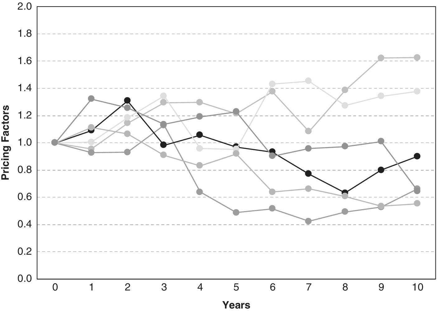
Figure A.9a Pricing factors for six future scenarios based on typical price dynamics: stock market (simulations based purely on the random walk).
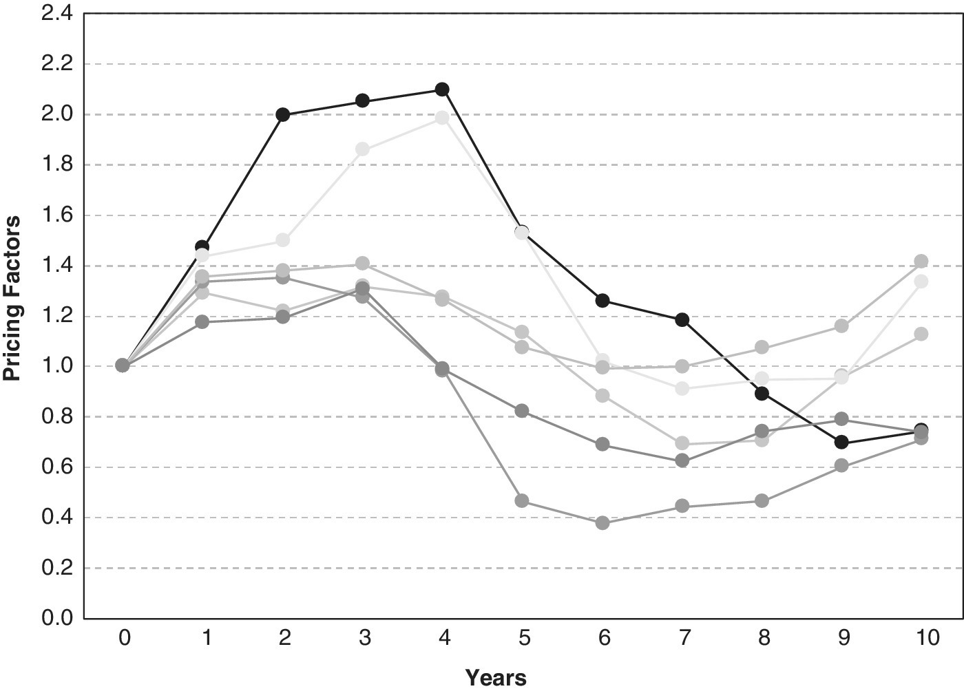
Figure A.9b Pricing factors for six future scenarios based on typical price dynamics: real estate (simulations based on random walk and cyclicality, mean‐reversion, and autoregression).
