21
Product Mix Flexibility: This Chapter Presents the Option to Change Product Mix, and Examines the Effect of Volatility on Option Value
This chapter focuses on a different type of flexibility—a product option as distinct from a timing option. We look at the flexibility to change the mix of products—specifically, to switch production between different types of buildings.
We see that product mix flexibility is essentially different from the timing options. It is not merely defensive in nature, but also offensive. Product mix flexibility is thus not redundant to the timing options, as the timing options are among themselves, as we saw in Section 20.5. Product mix flexibility adds distinct value to the timing options.
After we include the product switching option in our Garden City model, it is a good time to explore the general effect of market volatility on the value of development flexibility. We can explore this effect on a model that combines all three types of flexibilities: start delay, production timing, and product switching. We consider both the effect of volatility and of correlation between the product types on the investment performance characteristics of the Garden City project.
21.1 Product Mix Flexibility
Product options reflect flexibility in the quantity or type of real estate product(s) being constructed (see Section 13.4). In themselves, they do not affect the timing of the construction. They are “what” options, not “when” options. Product mix flexibility in its pure form would hold constant the total quantity of the product. It is thus different conceptually from expansion options (which we discuss in Chapter 23).
In the case of a project producing a large number of small, relatively homogeneous individual building units, such as the Garden City housing project, “product mix flexibility” refers to the developer’s ability to change the proportion of the total quantity of building production in each type of real estate product. For example, some housing units might be of different sizes, configurations, or fit‐outs, aimed at different submarkets of housing. Or, units might be aimed at different tenure markets, such as rental versus condominium.
In the case of projects producing one or more large buildings in more discrete quantities, product mix flexibility reflects the developer’s ability to change the type of structure on relatively short notice with little expense or operational difficulty. For example, the idea is to be able, perhaps just prior to (or even after) the start of construction, to switch the plans for a building from apartment to hotel, or warehouse to lab space, and so forth.
Product mix flexibility does not exist to a great degree in some, perhaps most, development projects. Developers may have to invest in substantial planning, specialized design, and other preparation to enable this type of flexibility. Is such extra planning and management worth it? The analysis in this chapter shows how to answer that question, and provides some suggestive results based on our Garden City example project.
21.2 Modeling the Product Mix Option
How can we introduce product mix flexibility into the spreadsheet‐based DCF valuation model? In essence, we model product mix flexibility in the same way as the production timing flexibility that we considered in the preceding three chapters. We formulate a decision rule in the spreadsheet DCF model. We base this rule on a decision criterion that is observable at the time when the option to switch products can be exercised.
The decision criterion typically compares the relative profitability between or among the types of products. In any given future scenario, in any given year, such profitability will result from the realization of the pricing factors based on our probability and market dynamics inputs.
Recall that, in the Garden City project, we identified two different types of housing units, which we labeled “Type A” and “Type B.” For simplicity of illustration, and to explore an archetypical result, we assume that the two types are completely interchangeable. That is, the developer can decide what type to sell each year, and then build this type during the following 2 years. Indeed, to consider an extreme case, analogous to our model of modular production timing in the previous chapter, we here assume that the product mix is all or nothing. We sell either only Type A or only Type B in any given year, and we can switch back and forth from one year to the next.
We use a simple decision criterion. In each year of the scenario, the spreadsheet compares the current price of Type A and Type B houses. Since, for simplicity, we assume that both types of houses have the same construction cost, this criterion effectively compares the current relative profitability of each type of housing product based solely on the relative demand for the two products, which underlies their respective pricing factor realizations. This is a logical basis for the product mix decision in any given year. (This decision rule is also admittedly myopic. It only considers a single year, rather than several. In that respect, it is analogous to the Simple Myopic Delay Rule for the delay option we used in the two previous chapters.)
In general, the analyst can also input a trigger value into the decision rule. For example, this might switch construction from Type A to Type B only if their difference in profitability exceeds the trigger percentage. That is, if the trigger is input is 10%, then:
- The switch to sell only Type A that year will occur only if Type A’s current price realization exceeds Type B’s current price realization by more than 10% of the base case average projected housing sales profit per unit for that year.
- Conversely, the switch will occur in the other direction, selling only Type B, if the Type A minus Type B profit realization falls below negative 10% of the base case profit projection for that year.
In fact, a trigger value of zero is optimal under the conditions set up for our stylized, archetypical analysis. Any other value would allow the sale of some less profitable houses. Our analysis thus sets the decision rule such that, each year, the developer sells only and entirely whichever type of housing is more profitable, which effectively equates to whichever type has the highest current pricing factor realization.
Our market dynamics assumptions create a high degree of contemporaneous cross‐correlation in the pricing factor realizations for Type A and Type B housing (see Section 17.1). In effect, we assume that these two products are very similar, and that their markets are highly correlated. But they are not perfectly correlated. To some extent, each type exhibits its own individual random walk and idiosyncratic noise elements. Specifically, our standard inputs for the Garden City project assume that each type of housing displays annual price volatility just under 20%, with a correlation between the two of around 80%. We vary these assumptions later, in Section 21.5.
Because the Type A and Type B housing pricing factors are not perfectly correlated, one type or the other will randomly turn out to be more profitable in any given year. Our option to switch the product mix responds to the random realization of this relative pricing history across the future scenario. While this model is clearly a simplified version of reality, it captures the essence of how product mix flexibility can work in a real estate development project that produces a large number of relatively small, homogeneous building units, especially if the design of the project allows it.
21.3 Value of Product Mix Flexibility
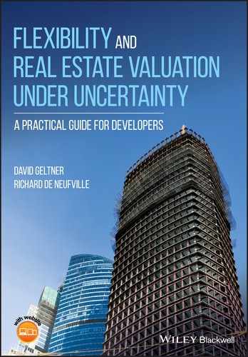
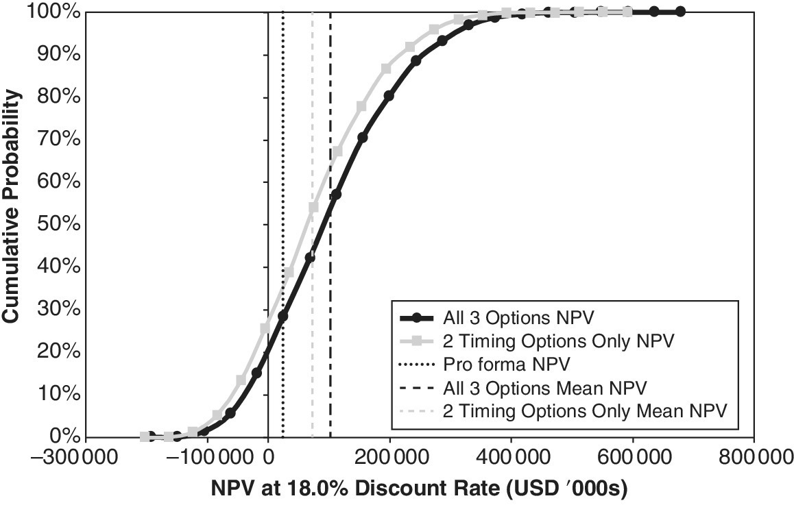
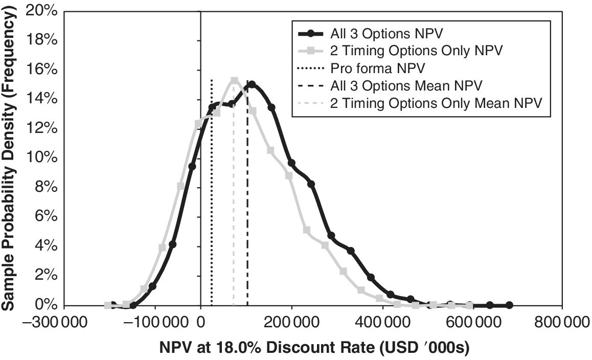
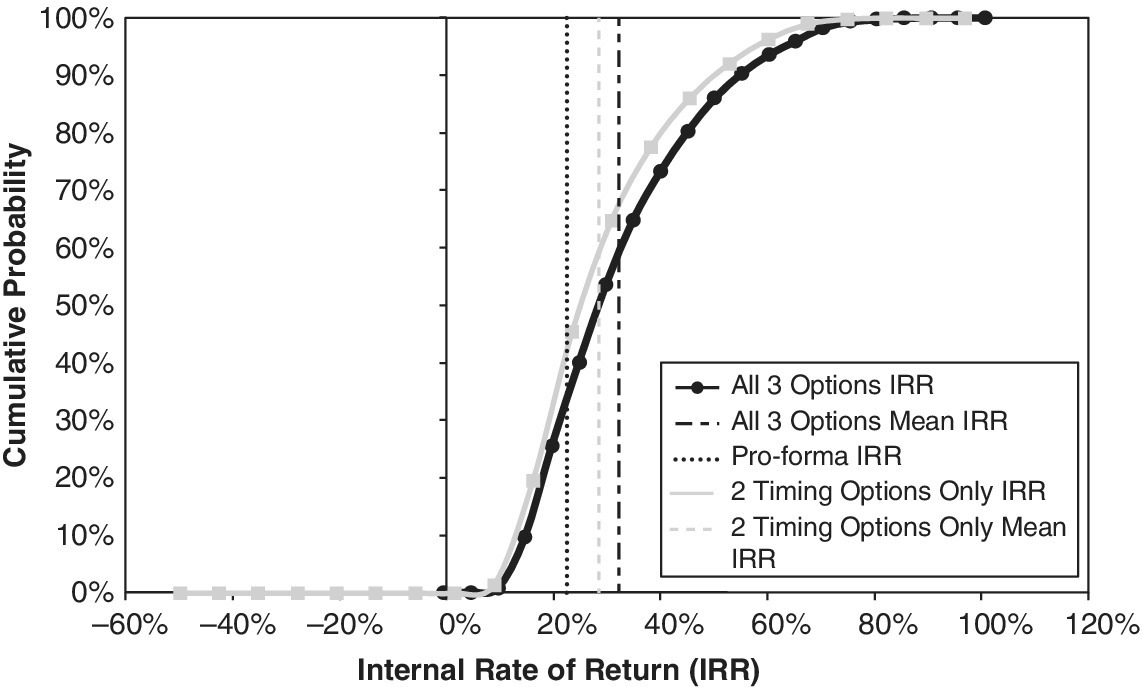
Figures 21.1–21.4 show typical target curves resulting from the Monte Carlo simulation of product mix flexibility in our example Garden City project. Two features are noteworthy.
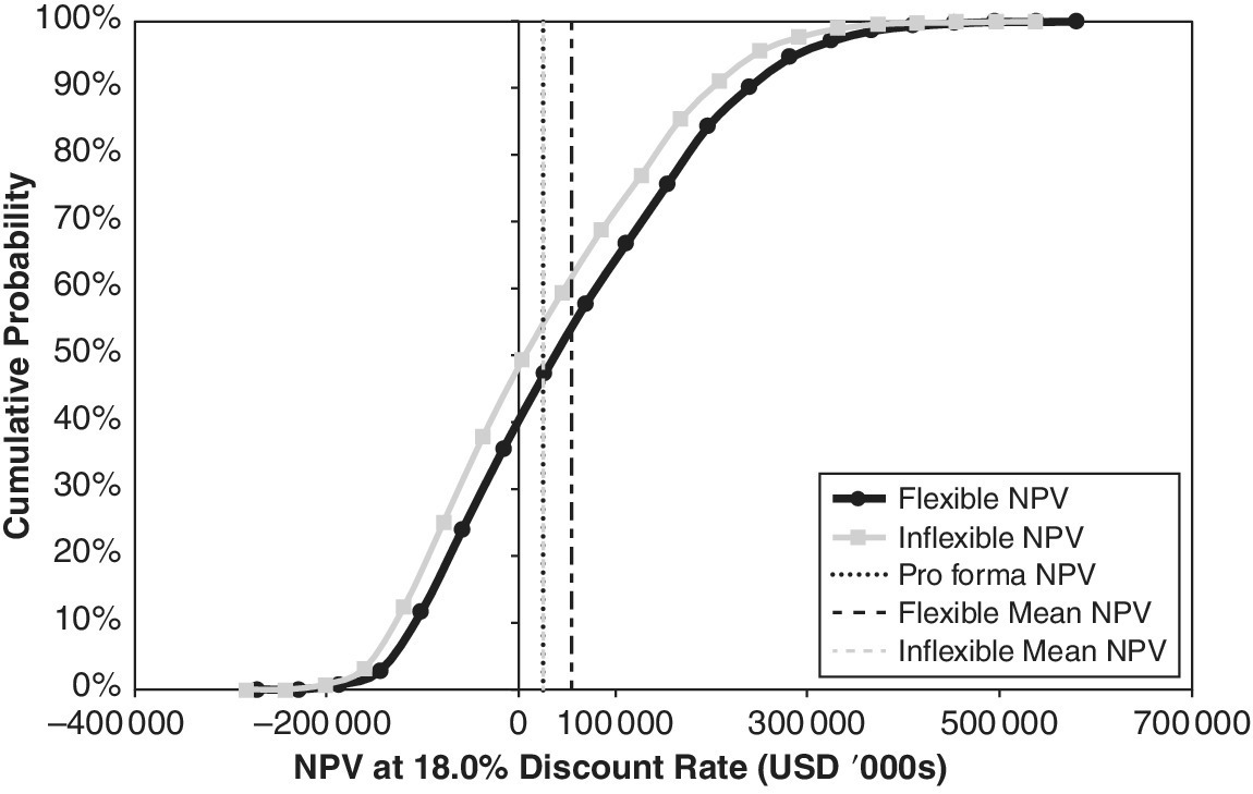
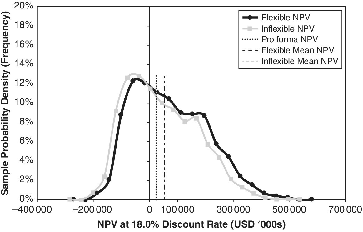

First, it is clear that the product mix flexibility adds value for investors:
- The expected NPV with flexibility is about $30 M greater than that of the inflexible project, equal to 13% of the pro forma valuation of the land, and over 3% of the gross PV of the assets to be built.
- The expected IRR increases over 500 basis points, to approximately 25% from 20%.
Second, the entire outcome distributions shift in the positive direction (to the right on the horizontal axis). The:
- Downside tail, 5% value at risk, of the IRR distribution rises approximately 700 basis points, from negative 19% to negative 12%.
- Upside tail, 95th percentile, rises a similar amount, from approximately 57% to 63%.
This shift of the entire outcome distribution is different from what we saw with the timing options in the previous three chapters. The timing options primarily only affected the downside outcomes. They were defensive delay options.
In contrast, the product mix option is both defensive and offensive. In effect, it is both a:
- Call on the product type being chosen, while simultaneously being a
- Put on the type being avoided.
The switching option lets developers both take advantage of upside opportunities and avoid downside outcomes.
It is instructive to compare the effect of the product mix flexibility with that of the timing flexibilities we discussed in Chapters 18–20, in each case quantified relative to the inflexible case in which no deviation is permitted from the base plan production. The increases in expected NPV from the various types of flexibilities by themselves are approximately:
- $30 M for the product mix flexibility (13% of land value);
- $45 M (20% of land value) for overall project start‐delay flexibility with the Simple Myopic Delay Rule (Chapter 19), or only $8 M with the Aggressive Developer Rule (Chapter 18);
- $25 M for modular production delay flexibility with the optimal negative 20% trigger (11% of land value), or $20 M with the neutral zero trigger level (Chapter 20).
As regards the expected IRR, each of the preceding options (the two timing options and the switching option) appear to add over 500 basis points under their best decision rule settings (for the Simple Myopic Delay Rule).
In terms of the future investment performance dispersion (a basic measure of risk) as measured by the simulated outcome standard deviation, the:
- Defensive timing options chopped off the downside of the distribution, and thus reduced the spread of the outcomes.
- Offensive/defensive product mix option shifted the entire outcome distribution right, but did not chop off any tail, and thus did not appreciably reduce the spread of outcomes or the overall investment risk.
The product switching and the timing delay options both imply significantly increased land value, but by rather different amounts and in different ways (downside tail versus both tails). Of course, these specific results apply only to our example Garden City project, with the admittedly somewhat extreme and archetypal definitions of the options that we are examining here for analytical purposes. And the results depend on the specific probability and price dynamics inputs that we have been using in the simulation. However, we constructed the Garden City example as a typical type of multiple‐asset development project, and we believe our pricing input assumptions are realistic for typical real estate markets. Most of the investment performance results are generally and qualitatively robust to reasonable variations in the price dynamics input assumptions, and not biased to be favorable for flexibility value.
The scatterplot in Figure 21.5 provides another perspective on the difference between the product mix switching and the delay options. For the timing options (see Figures 18.5, 19.5, and 20.6), the cloud of outcome dots showing how the IRR of the flexible case outperformed the IRR of the inflexible case, generally:
- Sloped downward from left to right;
- Was higher above the zero‐difference horizontal axis over the downside outcomes toward the left of the graph;
- Indicated some scenarios in which the inflexible project outperformed the flexible project, even if these scenarios were few and clustered in the upside of favorable project outcomes.
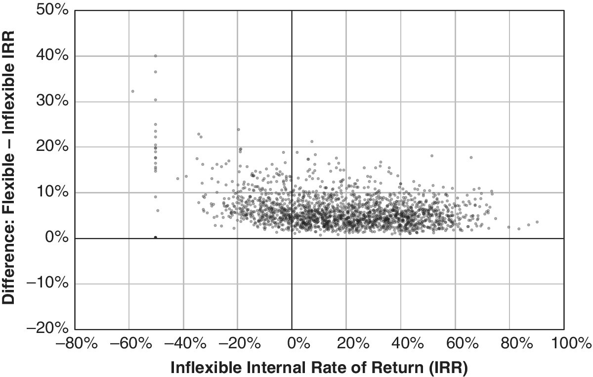
Figure 21.5 Scatterplot of IRR outcomes for product mix flexibility versus no flexibility at all.
By contrast, Figure 21.5 shows that the similar cloud of outcome dots for the product switching option is:
- Not sloped over the horizontal axis;
- Quite evenly above the horizontal axis, except for some (very few) extreme high outliers on the downside;
- Always entirely above the horizontal axis.
The dominance of the flexible case for the product mix option is a result of the zero trigger level. In effect, this steers the project toward always selling a greater proportion of the more profitable type of housing. Chance guarantees that it would be rare indeed for there to be an outcome in which the pricing factors were always identical between the two product types.
21.4 Effect of Combining Product Mix Flexibility and Timing Options
Our product switching option provides a fundamentally different improvement in investment performance than that provided by the delay options. It thus seems likely that the product mix option might combine more complementarily with the timing options. Recall that the two timing options, the start‐delay option (Chapters 18 and 19) and the modular production flexibility (Chapter 20), combined together largely redundantly (see Section 20.5). The overall investment performance with the two options together was hardly superior to that of the best of either type of timing option by itself, at least in terms of the central tendency of the result.
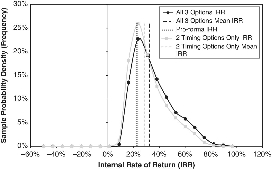
Now look at Figures 21.6–21.9. They compare the target curve outcomes for all three options together with the outcomes of just the two timing options together (using the Simple Myopic Delay Rule and optimum trigger values). Notice that the incremental effect of adding the product mix option looks very similar to the effect of that option by itself (compare Figures 21.6–21.9 with Figures 21.1–21.4). In other words, the product switching option has a largely additive effect on top of the timing options. It improves the:
- Expected NPV by about $30 M to approximately $102 M for the three options combined (over 30% increment in the pro forma land value of $225 M from Chapter 16);
- Expected IRR by slightly less than the effect of the option by itself, but is still significant, adding over 350 basis points, to around 32% for the three options combined;
- IRR 5% value at risk by about 150 basis points, to near 12.5% for the three options combined;
- IRR 95th percentile (upside tail) by some 500 basis points, and, in so doing, slightly increases the spread and standard deviation of the IRR distribution—however, without any negative shift in its downside tail.
21.5 Effect of Correlation in the Product Markets on the Value of Product Mix Flexibility
The value of product mix flexibility depends heavily on the covariance between the markets for the two types of real estate products. The greater the correlation between the two markets, the less valuable is the switching option, other things being equal (see Section 14.3). In our pricing dynamics inputs for the Garden City example, we have assumed a very high correlation between the two markets, with an annual price‐change correlation coefficient of approximately 80% (across time within a given randomly generated future scenario).
Figures 21.10–21.13 show the effect of varying this assumption, specifically of reducing the correlation from 80% to 30%, holding other things constant. The charts model the product switching option only, without the timing options included in the previous charts. The lower correlation provides the product switching option with more opportunity to improve the project value over the inflexible half‐and‐half base plan. This improvement occurs broadly over the range of project outcomes. (Notice how the target curves are almost uniformly right‐shifted over the project NPV and IRR results.)
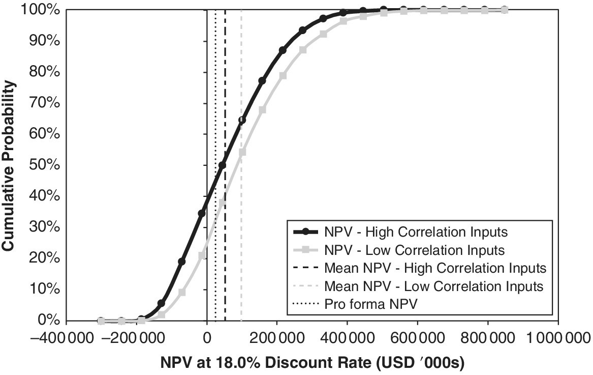
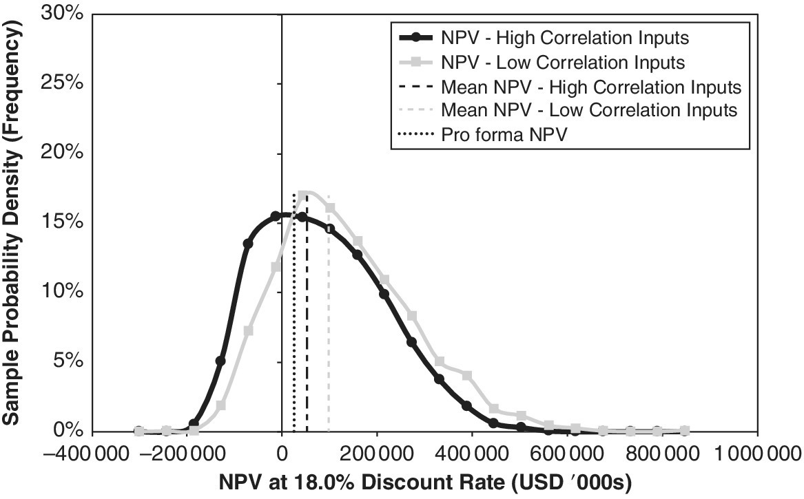
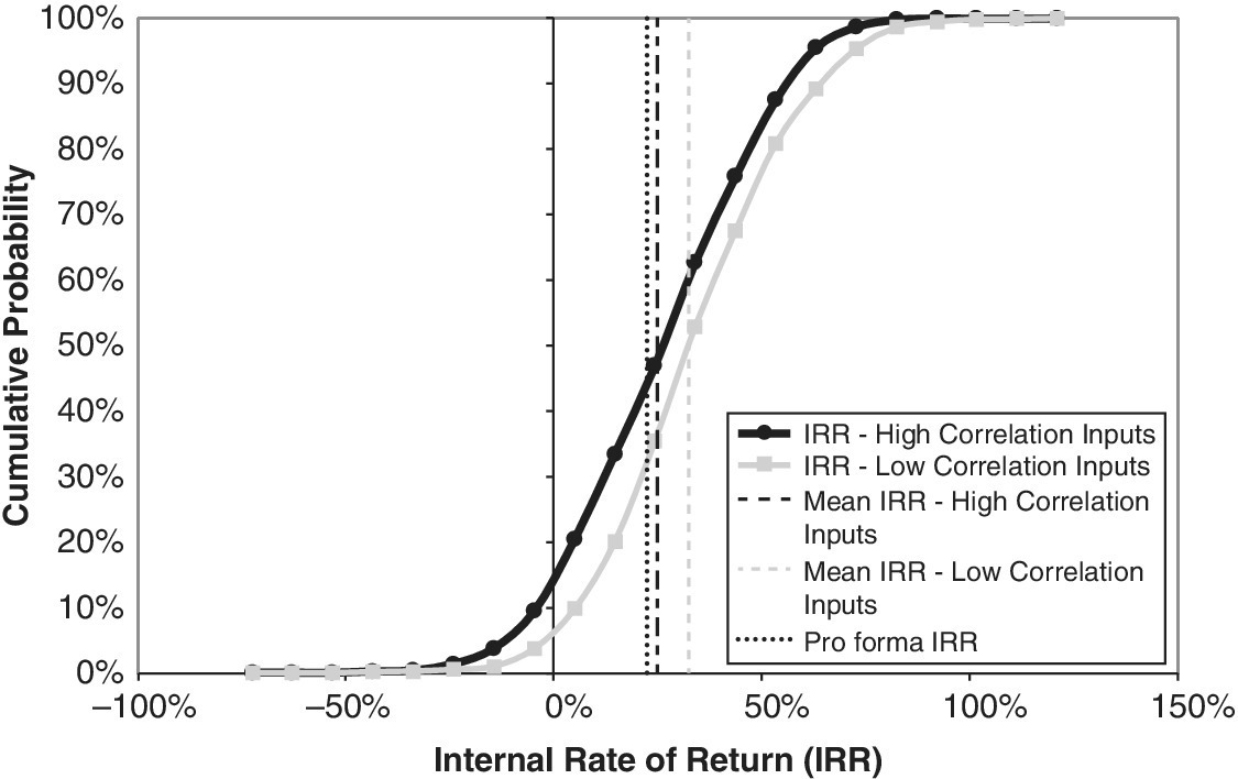
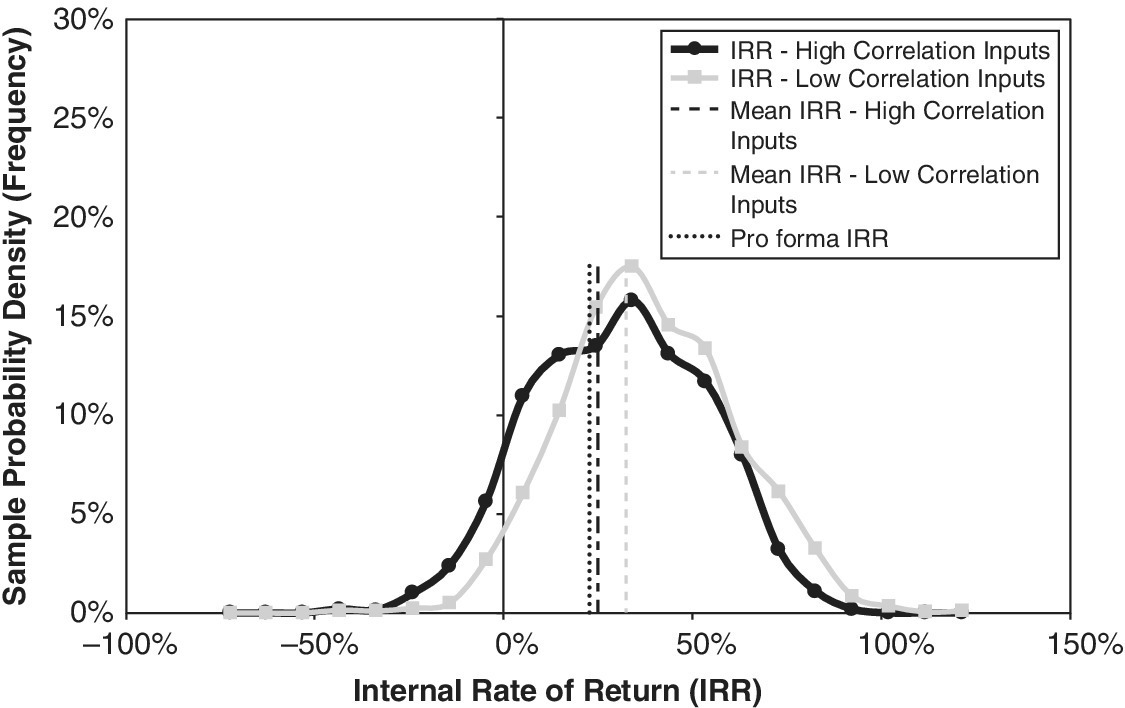
These comparisons make an important analytical point about how switching options add value. As noted, they provide simultaneous “puts” and “calls.” However, in reality, it may be unlikely that two types of real estate products that could be easily substituted for one another within the same project would have a price correlation as low as 30%.
21.6 Effect of Volatility on the Value of Flexibility
Now that we have covered the two timing options and one product option in some depth, this is a good time to step back and explore an important principle of option valuation. The greater the future uncertainty, the more valuable the options become. This is due to the “all gain and no pain” feature of options’ right without obligation. Regarding real estate developments, the magnitude of the real estate market price volatility reflects the amount of uncertainty. Options enable the developer to take advantage of upside opportunities and/or to avoid downside outcomes. When we discussed this general principle in Section 12.3, we did so qualitatively, and not quantitatively. So now we ask: How valuable is this favorably asymmetric payoff ability that options have in a typical real‐world development project? Our Garden City model allows us to explore this question.
Figures 21.14–21.17 show the effect of two different assumptions about product price volatility on the outcomes resulting from combining our three options together: start‐delay flexibility, modular production timing flexibility, and product mix flexibility. The black curve assumes real estate market price volatility of approximately 23% per year. The gray curve assumes volatility of about 17% per year. All other assumptions are the same as in our previous analysis. This range is plausible for property assets in the United States, and we used the same volatility assumptions in Figures 17.6–17.9, which showed the effect on project outcomes without flexibility. (In general, our assumption has been relevant volatility of around 20%. Keep in mind that the relevant volatility is not that of an index or market aggregate, but for the individual Garden City built property, including its idiosyncratic risk.)
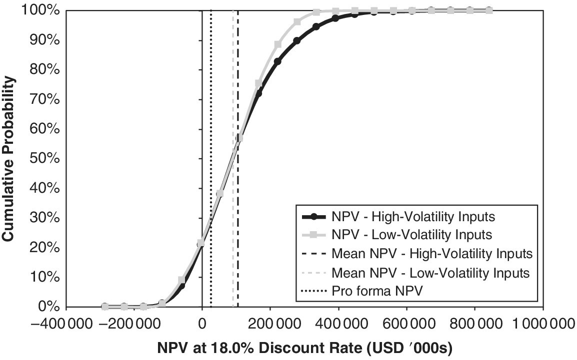
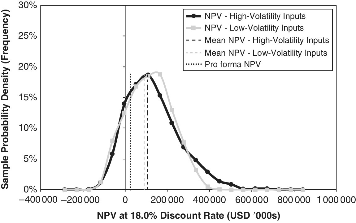
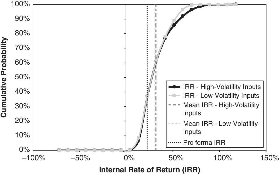
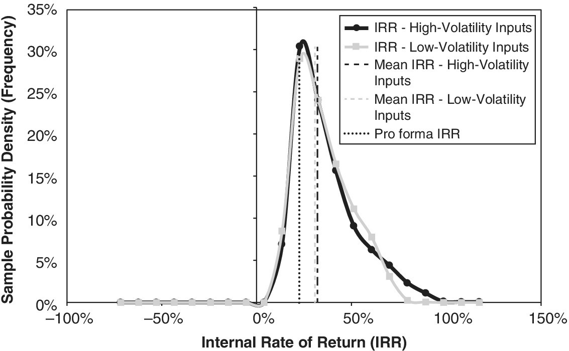
The ex‐post mean NPV is around $89 M for the low‐volatility assumption, and $105 M for the high‐volatility assumption. The central tendency of the outcome distributions suggests that the high‐volatility case increased the value of the combined options, adding around $15 M to the expected NPV, an increment of almost 7% of the land value, compared to the low‐volatility case. This contrasts with the situation without flexibility. In that case, the expected NPV and IRR of the Garden City project is not significantly different in the two volatility scenarios, although the standard deviations of the possible outcomes is, of course, greater in the high‐volatility environment (see Section 17.4).
It is important to note that we are assuming the same present value of the built project, across the two volatility assumptions, to see the pure effect of volatility, holding all else constant.
As you can see from the target curves, the increase in land value accompanies a slight increase in the outcome range, or risk, in the project value. The standard deviation of the project’s future realized IRR increases from about 15%, with 17% volatility in the built property, to about 17%, with 23% volatility in the built property.
While greater market volatility in real estate clearly tends to increase option value (holding other things equal), it is interesting that the magnitude of this effect is not very large over the likely typical range of volatility in real estate markets.
The curves in Figures 21.14–21.17 suggest that the increased value of the options with greater volatility is due largely to a right‐shift in the upside outcomes, the right‐hand tails of the distributions. The defensive delay options cut the left‐hand tails, but higher volatility spreads these tails and offsets this effect to some extent. In short, the delay options shift the left‐hand tail to the right, but the greater volatility shifts the left‐hand tail to the left. The two effects largely cancel each other out, at least when combined with the product mix option.
21.7 Conclusion
This chapter explored product mix flexibility, or the building type switching option, in our example Garden City project. We saw that such a product option adds significant value to a project. We also saw that, being both an offensive and a defensive option, it adds value rather differently from the purely defensive delay options discussed in Chapters 18–20.
We also saw how the product switching option is complementary or additive to the timing options. We showed how correlation in the markets for the alternative real estate products affects the switching option value.
Finally, we demonstrated the effect of volatility on the value of options in a typical real estate development project. Other things being equal (importantly, the value of the property assets to be built), increased volatility in the product markets implies greater option value. However, it seems that this option value is not highly sensitive to the likely range of volatility in typical real estate markets, at least as we have modeled these values in our simulation analysis.