This chapter presents an initial example of how we can identify hidden value using the DCF model to analyze scenarios. It provides a first demonstration of the value of flexibility. We quantify the added value we can obtain by modeling our management of properties to respond to downside and upside contingencies. The example we use is a simplified consideration of when to resell the property that we’re evaluating.

4.1 Discounted Cash Flow Scenario Analysis

Let’s now look at more than just the mean of the future cash flow, more than just the single‐stream pro forma. We can learn a lot by looking at what might actually occur in the future. A good first step for doing this is to think about future cash flow “scenarios” rather than just a single expectation. A scenario analysis can reveal important management possibilities or dangers. This enlightenment can lead the analyst to revise the original pro forma or asset valuation, especially (perhaps) from a private valuation perspective.

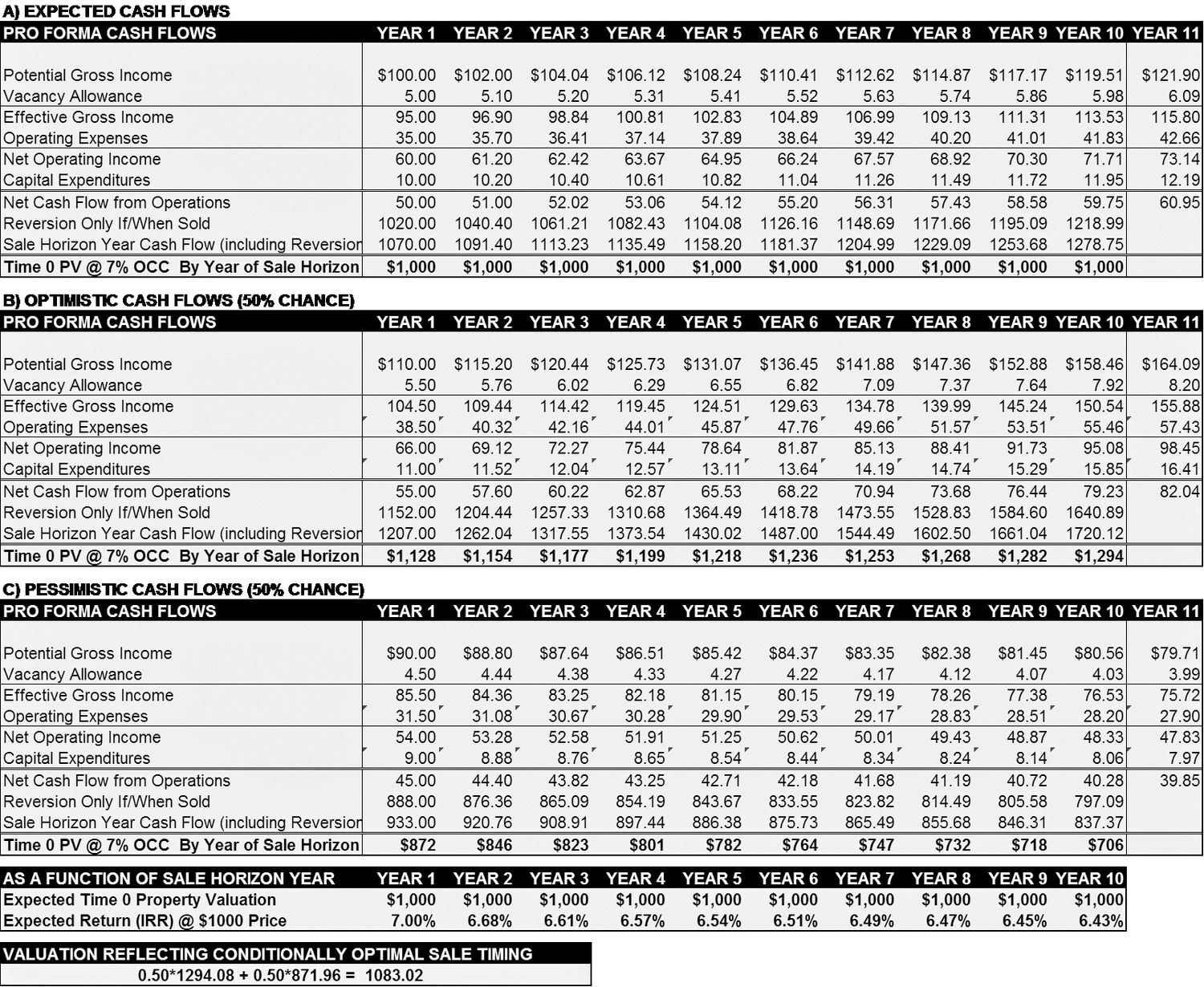
Let’s take a simple example that builds on the DCF for our example rental property. Table 4.1 shows three DCF pro formas.

• In the top panel, Panel A, the numbers are the same as in the original DCF (Table 1.1). As indicated in Section 3.3, its cash flow projections should be the expectations, the average of future cash flow possibilities in each period.
• Panel B represents a future, optimistic scenario, with a 50% chance of happening. In this example, we suppose that there are only two possible future scenarios, equally probable as of Time 0. For example, suppose the rental property could be near the site of a prospective attractive development (for example, a new metro station), with a 50:50 chance of going forward. Panel B assumes that the new development goes forward and that rents in the property we’re considering will be high. Compared to the DCF in Panel A, the optimistic scenario cash flows start out $10 higher in Year 1 and subsequently grow faster.
• Panel C represents the pessimistic scenario where the new development doesn’t occur. Compared to Panel A, rents in the property start out $10 lower than the expected value and decline over time.

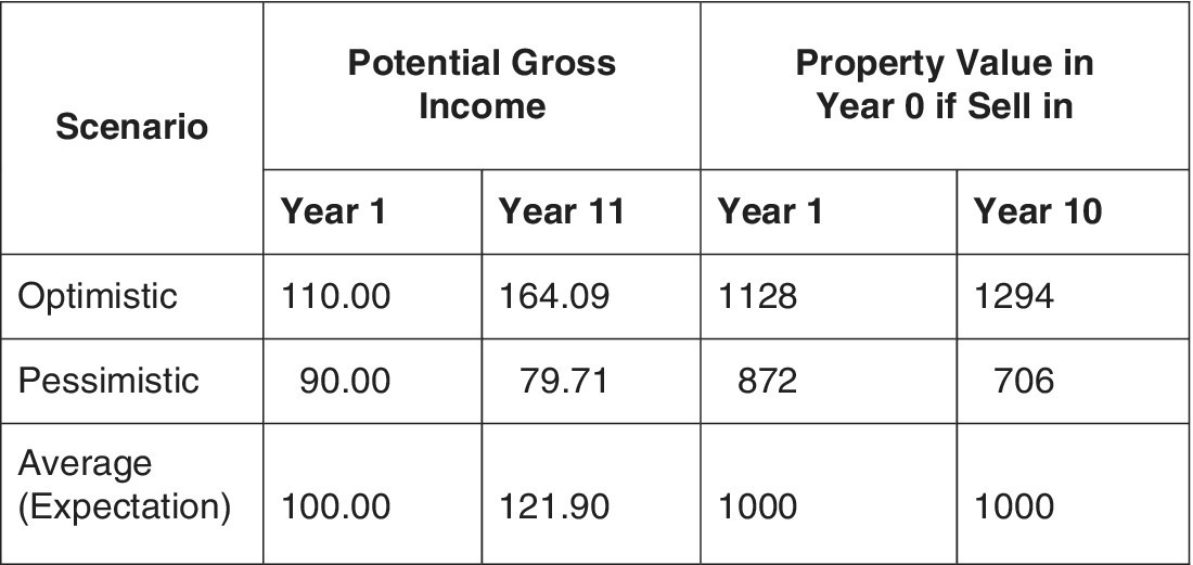
Note that the two scenarios average out exactly to the entries in Panel A. Thus, Panel A is the true expectations, the unbiased projection of the future possibilities, like what a good traditional DCF pro forma should represent. To facilitate the discussion, we’ve summarized the key aspects of the two scenarios in Table 4.2.

4.2 Scenarios Affect Value

The scenario that happens will affect the property value. We can quantify this effect exactly in the present value as of Time 0, the time of the analysis, assuming the 7% discount rate remains the correct OCC in both scenarios. (This is plausible, since that OCC did not presume any particular future cash flow path, but simply recognized that the future is risky.)

Under the optimistic contingency, the present value of the property as of Time 0 would:

• Be $1128 if it would be sold at the end of Year 1. This includes $55 of operating cash flow for Year 1 plus the reversion of $1152 at the end of Year 1, all discounted for 1 year at 7%.
• Increase the longer we plan to hold the property, reaching Time 0 present value of $1294 for a planned 10‐year holding period.

The opposite will occur under the pessimistic contingency. In that case, the present value of the property as of Time 0 would be only $872 if we plan to sell it at the end of Year 1, but would decrease even further the longer we plan to hold onto the property, falling to $706 if we plan to hold it for 10 years.

It is important to note that the traditional single‐stream DCF valuation represented by Panel A, based on the unbiased cash flow expectations, gives the same $1000 present value as of Time 0 as the expected present value implied by the 50/50 average of the two scenarios. For example, if we plan to sell at the end of Year 1, the expected present value of the property as of Time 0 is the 50:50 probability times the value of each scenario at the end of Year 1:

Moreover, this is true regardless of when we might plan to sell the property (that is, no matter what our valuation analysis time horizon is). For example, if we plan to hold for 10 years, we also get Time 0 present value:

It is important to note that the scenario that happens has implications for management decision‐making. Investors have the flexibility to decide when to sell. They can wait and see which scenario happens, and then make the value‐maximizing resale timing decision. Viewed from the present (Time 0), it would make most sense to:

• Hold the property for as long as possible, conditional on the optimistic scenario happening, or at least for the full 10 years in the traditional 10‐year horizon analysis, BUT
• Sell the property quickly, conditional on the pessimistic scenario happening, as that will maximize the present value.

This flexibility breaks the symmetry in the present values of each scenario. It leads to an actual, unconditional present value for the investment as of Time 0, differing from the Time 0 expected present value of the two scenarios (the $1000), owing to the effect of management flexibility.

This example is very simplistic, but it makes a general point: investors and managers can choose to act differently in response to circumstances over the course of the investment lifetime, and this can affect the value of the investment. The single‐stream, traditional DCF model can hide this fundamental and important fact.

4.3 Flexibility Has Value

We can quantify the value of the project recognizing its flexibility to time the resale. We do this by taking the expected value of the two possible outcomes under their value‐maximizing management decisions about the resale timing:

• $1294 for the optimistic scenario (sell in Year 10), and
• $872 for the pessimistic scenario (sell in Year 1).

As those scenarios are equally likely, the present value of the investment in the property, ex‐ante as of Time 0, and recognizing management’s flexibility to time its resale, is:

(4.1)

In other words, the investor’s ability to time the resale of the asset means that the property with flexibility is worth more than the $1000 present value we estimated using the traditional, single‐stream DCF model, even though that model here represents a correct, unbiased expected cash flow projection!

The value of the flexibility itself is the difference it makes to a project:

(4.2)

In our present, very simplistic example, this is:

(4.3)

If the investor had no resale timing flexibility, he or she must sell at the end of Year 10 (or any other year fixed in advance); then, the present value of the investment is indeed $1000. But if the investor has the flexibility to make the value‐maximizing resale, then the present value of the investment is $1083.

Let’s take a moment now to make the crucial point that flexibility has value, as the preceding example reveals. This general point is central to this book. If we have flexibility, we can wait and see which scenario happens, and then make value‐maximizing decisions. We can thus unlock important value.

This book is all about identifying desirable forms of flexibility and valuing them. It can be useful to know this “extra” value. It can perhaps suggest actions to enable or implement such flexibility. One can consider whether a particular flexibility is worth its cost, if indeed there is any cost to acquire or enable the flexibility. We also note that added flexibility does not always add value (see Box 4.1).

By contrast, we should note that the traditional DCF model tempts users to ignore or downplay the value associated with flexibility in the presence of uncertainty. The traditional DCF model does not allow us to explore possibilities that might exist, or how we might intelligently react to what can happen as the project or investment develops over time. It does not quantify the value implications that flexibility holds for the investment at Time 0, the time of the analysis or decision.

To explore these possibilities of dealing with uncertainty, we have to expand the DCF analysis. In our example, we:

• First represented the uncertainty by scenarios (optimistic and pessimistic cash flows), which took the place of the single‐stream, traditional DCF model.
• Then examined the implications within each scenario of the investor’s flexibility—in this case, the flexibility to choose the time of selling the property.

This is the pattern we use throughout the book: we expand on DCF analyses to quantify the value of flexibility.

4.4 Conclusion

Decision‐makers in real estate development and investment projects usually have various types of flexibilities regarding what actions they can take and when to take them. They can and will respond to the actual scenarios as they happen. Recognizing this explicitly in valuation can change our understanding of the value of investments. It can also have implications for the design and management of projects.

This chapter presented a very simplified illustration of these points. In the real world, the future is not nearly as simple as the example in this chapter, and decision‐makers may not always respond optimally, either in prospect or when viewed in retrospect. Subsequent chapters will demonstrate more realistic models. But the key point is that we can improve decision‐making and fundamental understanding and valuation by explicitly considering, and modeling, uncertainty and flexibility. The remainder of this book presents an approach to help you do that.