
23
Optimal Phasing: We Now look at Adding Phases, Delineating Phases, and Distinguishing them from Expansion Options
In this last chapter of our exploration of the value of flexibility in real estate development projects, we tie up a few loose ends having to do with project phasing. The overall question is: What is the best way to design and program the phases in a project?
- We begin with a natural follow‐up to Chapter 22. Since it is good to divide the project into two sequential phases, would it be even better to have three phases (holding the overall scale of the project constant)?
- Second, how should we delineate between phases? That is, how much of the project should we put in one phase versus another, especially in the first phase versus later phases?
- Finally, our analysis of phasing begs a broader question—one that relates back to our typology of development flexibility, introduced in Chapters 13–15. What is the difference between a later “phase” versus what we described as an “expansion option”? We shall see that the key is in the designation of the project’s “base plan”—that is, how committed the developer is to carrying out which potential components of the project.
23.1 Effect of Increasing the Number of Phases
We begin by taking a logical next step from Chapter 22, where we examined a two‐phase version of the Garden City project. What if we re‐cast the Garden City project to be essentially the same, except now we divide it into three phases instead of two?
Let’s examine this issue on the same basis as before. We’ll continue to examine phase start‐timing flexibility only in the subsequent phases, after the first phase, requiring the first phase to start immediately as we did in Chapter 22. The latter two phases must follow sequentially, but the start of either Phase 2 or Phase 3 may be delayed. We apply the same start‐delay decision rule and trigger value as with the two‐phase project in Chapter 22.
We find that the additional phase clearly adds value. The increase in ex‐post mean NPV is strongly statistically significant in our simulations. The rationale is intuitively clear: three phases (with two able to be delayed) has more flexibility to time production than two phases (with only one phase able to be delayed). Our simulations substantiate this point. With the first phase committed to start without delay, the:
- Three‐phase project has an average overall completion delay of less than 4 years (reflecting delay in either Phase 2 or Phase 3, or both);
- Two‐phase project faces an average completion delay of about 2.5 years.
Importantly, however, the additional value of adding a third phase is not great; it is of minor economic significance, at least in the case of our archetypical Garden City project. It is much smaller than the value of introducing the second phase compared to no flexibility at all. (And recall that adding a flexible second phase added much less value than allowing the entire project to be flexible, as in Chapter 19.) Comparison of the three‐phase versus two‐phase version of Garden City reveals the following:
- The mean NPV increment due to the third phase is only about $2 M (over the two‐phase plan) in a project of $815 M gross present value and $170 M land value. The expected IRR increases by less than 50 basis points as compared to the two‐phase project.
- By comparison, the mean NPV increment due to the second phase was $12 M (in the absence of start‐delay flexibility for the whole project), and the expected IRR increment was almost 400 basis points (see Chapter 22). And start‐delay flexibility for the whole project as a single phase added $45 M (20% of land value) to the inflexible mean NPV, and 700 basis points to the expected IRR (see Chapter 19).
Intuitively, these results would seem to reflect a general rule. Adding more phases (hence, more production timing flexibility), holding overall project scale constant, should increase value, but at a diminishing marginal rate as one adds more phases. The fact that breaking a fixed project into an additional phase adds only a little to the value of flexibility in the project is not surprising after what we discovered in Chapter 20 about the redundancy of production timing options. We noted in Section 20.5 that, if the project has overall start‐delay flexibility, adding subsequent production timing delay flexibility does not add as much value as the subsequent production timing flexibility would add by itself if there were no overall start‐delay flexibility. Our finding here is similar, again reflecting some redundancy in the options that allow delay of production.
The scatterplots in Figures 23.1 and 23.2 compare the three‐phase and two‐phase results to each other. Because these projects have slightly different pro formas with different NPVs and IRRs, we cannot directly compare their results—it would be an “apples versus oranges” comparison. The appropriate comparison is each project’s difference from its inflexible case. Thus, whether by the NPV or IRR performance metric, the comparison of interest is a “difference of differences.” This is the comparison metric shown in the Figures 23.1 and 23.2:
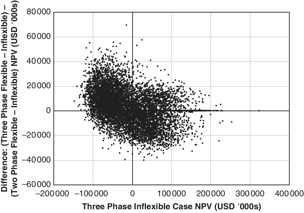
Figure 23.1 Scatterplot comparing NPV for three versus two phases.
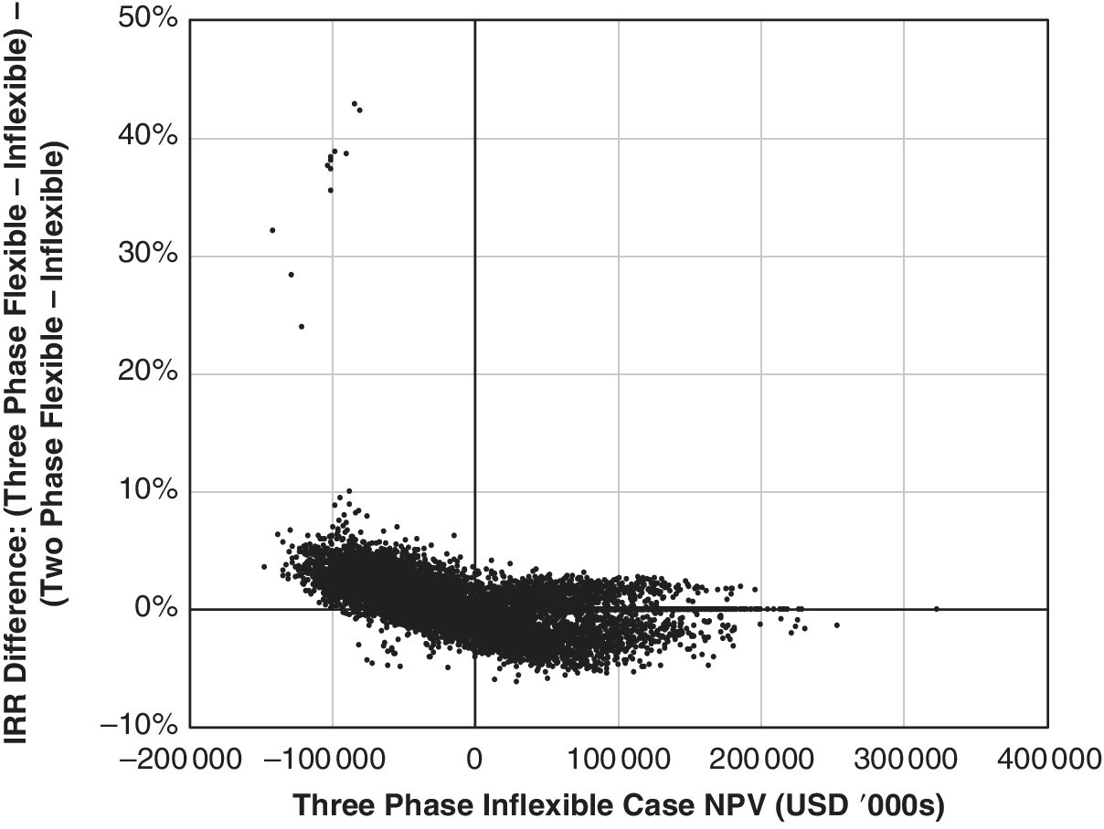
Figure 23.2 Scatterplot comparing IRR for three versus two phases.
In Figures 23.1 and 23.2, the dots:
- Above the horizontal axis (zero‐difference line) are scenarios (trials) in which the three‐phase project beat the two‐phase project;
- Below the axis are outcomes in which the two‐phase project beat the three‐phase project;
- Exactly on the axis (no difference) are outcomes in which no delay option was triggered, so neither phasing scheme gained more than the other from such flexibility.
Whether by the NPV or IRR metric, the three‐phase project beats the two‐phase project in over 40% of the outcomes, almost twice as frequently as the reverse occurs. However, there is evidence that adding phases, holding overall project scale constant, is a declining marginal benefit in terms of investment performance.
The third phase adds value defensively, as we would expect, by reducing downside exposure. It provides more flexibility to delay the project in bad market conditions, and thereby avoid or mitigate losses. The scatterplots in Figures 23.1 and 23.2 indicate this through their generally downward sloping shape from left to right.
But this downward slope is only slight, and is almost swamped by the random dispersion in the outcomes. Unlike some of our previous results in earlier chapters, we do see a non‐trivial proportion of dots in the lower‐left quadrant, indicating that sometimes the two‐phase project did better when the project overall was doing poorly. The “insurance” function of the additional flexibility is more limited with the marginal contribution of the third phase.
23.2 Principles for Optimal Phasing
The previous discussion begs a complementary question. Suppose we fix the number of sequential phases in a project: What is the best way to assign physical components of the project to those phases? In other words, given a set of physical elements in an overall project (a “base plan”), how should we group them into sequential phases? In effect, how should we delineate between one phase and another?
The two questions together—the question of the optimal number of phases (Section 23.1) and the question of what to put in each phase (the present section)—define the overall question of optimal phasing for a development project.
Of course, there is no completely general answer to this question, as each project is unique. Specific design and programming issues, physical and economic relationships between the project elements, will be important in defining the phasing of any given project. But we can use the simulation modeling of our Garden City example to identify some plausible principles, or at least some common‐sense intuition, answering a basic question of optimal phasing: How much of the project should we put in each phase?
We derive the principles from a study of the range of possibilities in terms of:
- Types of projects (in terms of temporal profiles of production);
- Possible divisions into phases;
- Timing with respect to the real estate cycle.
Our study considers the entire range of possible combinations, but it does not go into excessive detail. The idea is not to be comprehensive; it is to gain insight. As always, we want to “see the forest through the trees.”
First, concerning the type of projects, we model the essence of the physical production of the project by defining four archetypical project base plan profiles (Figure 23.3). These cover possible differences in:
- Duration of project: 5 and 10 years. These would seem to represent a good range of project duration for major real estate development projects.
- Temporal distribution of production: front‐loaded, with a peak of work near the beginning of the project (like Garden City of Chapter 16), or uniform over duration (like Garden City of Chapter 22). Again, these would seem to span the main typical patterns.
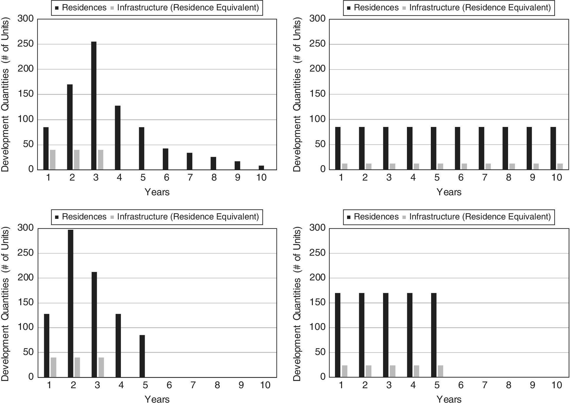
Figure 23.3 Four archetypical base plan temporal production profiles for major real estate development projects.
These base plans, of course, do not depict any production delays caused by the ex‐post exercise of timing flexibility.
Second, to explore the optimal delineation of product to phases, we consider the simplest case, in which the project can have at most two phases. Limiting the analysis to two phases provides a parsimonious way to develop the basic intuition that likely applies more broadly. We compare all possible ways of assigning the project’s production to the two phases. The comparison in all cases is against the benchmark performance of a project with no phasing and no delay flexibility.
Against this benchmark, we consider all possible schemes for dividing any of the four profiles of Figure 23.3 into two phases. In each scheme, the first phase has no timing flexibility; it must start immediately and proceed to completion without delay. Within this framework, “Scheme 1” places the first year’s base plan production in Phase 1 and the rest of the project in Phase 2 (the phase that does have start‐delay flexibility). “Scheme 2” places the first 2 years’ production in Phase 1 and the rest in Phase 2. And so on. The 5‐year projects (whether front‐loaded or uniform profile) have four such two‐phase schemes (up through “Scheme 4,” which places only the fifth‐year production of the base plan into the second phase). Similarly, the 10‐year projects have nine such possible two‐phase schemes, up through “Scheme 9.” In addition, we define a “Scheme 0” for each of the four base plan profiles, in which all of the project is put into a single phase that does have start‐delay flexibility, like the option examined in Chapters 18 and 19 for Garden City. Relative to the benchmark, we therefore have five phasing schemes for each of the two 5‐year project base plans (front‐loaded and uniform), and 10 phasing schemes for each of the two 10‐year project base plans. This framework provides a comprehensive typology for project phasing, given a maximum of two phases.
Third, we need to see how the phasing schemes and base plan profiles interact with the real estate market cycle. Logically, the key driver of the relative success of the alternative phasing schemes would be how the phasing interacts with the real estate market swings in the different base plan profiles—the ups and downs in the market pricing factors in our simulation scenarios relative to the pro forma projections. This can be most parsimoniously represented by a deterministic cycle. We implement this aspect of the analysis by considering:
- Market cycles of different lengths; and
- Projects starting in different phases of the cycle.
We consider four deterministic cycles of different period lengths: 5, 10, 15, and 20 years. These periods range from being equal to the short (5‐year) base plans or half the duration of the 10‐year base plans, up to four times the duration of the 5‐year plans and twice the duration of the 10‐year plans. For each of these cycle periods, we test four different phases of the market cycle as of the beginning of the project (“Time 0”): mid‐cycle headed up, peak heading down, mid‐cycle heading down, and bottom headed up.
In short, we look comprehensively across all the possible ways in which different phasing schemes could perform, interacting with the market cycles, for the four different base plan production profiles. We replicate the Garden City analyses that we have reported in Chapter 22 and Section 23.1, using the same assumptions concerning the amplitude of the cycles, the discount rate, and the delay decision rule.
We can distill the results of our analysis into a general rule: Make as much of the project as flexible as possible, as early as possible, but think about the implications of the market cycle. In more detail, we propose a set of principles:
- As a rule, it’s best to make as much of the project subject to start‐delay flexibility as possible. Thus, the scheme that has only one phase with full start‐delay flexibility often looks best.
- The major exceptions to the preceding general rule are:
- If the project base plan profile is front‐loaded and lasts longer than the market cycle, it’s best to put some of the project into a flexible second phase (unless you are at the market cycle peak, in which case you need to do it all in one phase, starting immediately). The idea is to avoid doing the project during down markets and to concentrate it as much as possible into the up‐market part of the cycle.
- If the initial phase cannot have start‐delay flexibility, then it’s best to minimize the amount of the project in the inflexible first phase. This is because, as we have seen throughout the book, flexibility has value, and more flexibility has more value.
- The preceding rules do not apply to a uniform base plan production profile for projects spread out over a very long time. Their long duration and uniform production “diversify” profitability across the cycle. What they lose in one part of the cycle, they gain in another. Such projects gain relatively little from production timing flexibility, and could, in fact, lose from such flexibility if they start during a recessionary period.
These principles for optimal phasing are neither complete nor comprehensive—nor are they definitive. They derive from a simple, stylized study. But they seem to be consistent with common sense and basic intuition. Combined with our prior findings in Sections 20.4, 21.4, 22.5 and 23.1, we offer these principles as a basis for thinking generally and systematically about the value of timing flexibility and the optimal phasing of real estate development projects.
23.3 What Is the Difference between a Phase and an Expansion Option?
This brings us to the last question that we will take on in this book regarding flexibility in real estate development projects. In Chapters 13–15, we introduced a typology of real estate development project flexibility, and generally distinguished between expansion options and phasing flexibility. We described:
- Phasing flexibility as a type of production timing option, essentially defensive in nature, reflecting the ability to delay the start of a phase of the project if market circumstances are unfavorable;
- Expansion options, whether horizontal or vertical, as product options akin to a call option, an “offensive” type of flexibility aimed at enabling the developer to build additional products in response to upside opportunities.
In some sense, we presented phasing flexibility and expansion options as opposites. In our specific simulation modeling of the example Garden City project in the past chapters, we have provided examples and analysis of phasing options. And we provided an example of one product option: building type mix flexibility. But we have not provided an example analysis of an expansion option. Have we left something out?
We think not. When you get right down to it, in terms of formal, analytical modeling, an expansion option is not essentially different from another (later) phase of the project. We can apply the same type of model and simulation analysis to an expansion option as for the phasing options that we illustrated in this and the previous chapter. This is because the distinction between phases and expansions is conceptual rather than formal or mathematical. The distinction reflects the developer’s perspective and the corresponding planning decisions. For example, we noted in Chapter 12 that the Bentall 5 vertical expansion in the Vancouver building could be viewed as a defensive (“put” type) option to delay (or abandon) the top floors of the planned building—or, equally, it could be viewed as an offensive (“call” type) option to add five more floors to the base plan. Either way, it is the same option from the perspective of formal modeling and simulation.
Therefore, we may define the essential difference between a later sequential “phase” and an “expansion option” as being that a:
- “Phase” lies within the original commitment for the project, what we have been calling the “base plan”; and an
- “Expansion option” lies outside or beyond that base plan.
Thus, the distinction between an expansion option and a later phase lies in the planning decision of what to put in, and what to leave out of, the “base plan.” This decision will reflect basic and specific physical, legal/regulatory, political, economic, and marketing considerations about the project. It will also reflect the production capacity of the developer, and the limits of the financing sources for the project. Crucially important may simply be the amount of demand foreseen for the project within a reasonable period. It may also be valuable to wait and see how the base plan turns out, to see what we learn about the market as a result of the performance of the base plan, before going very far in the planning or design of an opportunity for additional product on the site.
The difference between “base plan” and “expansion option” would be that the developer is committed to the base plan but not necessarily to the expansion. Operationally, the developer (and financial backers) are “very committed” to producing the entire base plan quantity, by some point in time, though not necessarily in the originally planned base plan time frame (as we have seen how valuable delay flexibility is). Perhaps we could even quantify this notionally as reflecting, say, “greater than 90% probability” that the developer will fully complete the base plan. The developer would probably have largely lined up financing for the base plan, and has relatively complete and detailed designs and drawings for it.
In contrast, while developers may hope, and perhaps even expect, to realize an available expansion option someday, they have markedly less commitment and planning for it as of the time they start the project. Again, at a notional level, perhaps we could say something like there is “a 40–60% probability” that an expansion option will ever happen, at least within the foreseeable future. It would not make sense to spend too much time and effort yet on lining up financing or completing detailed plans for such a future option.
In terms of the formal modeling and simulation analysis, there should therefore be only a single but important difference between the analysis and valuation of an expansion option and that of the base plan. To reflect that the expansion option is significantly less likely to happen, we should apply different real estate market pricing dynamics to the real estate products included in the expansion option. We would need to have separate inputs of the dynamics and uncertainty governing the pricing factors for the expansion option simulation, compared to the base plan simulation. For example, in our simulation of delay flexibility and phasing schemes in Garden City, we find that we virtually never abandon the project and almost never fail to complete it. In contrast, a realistic simulation including an expansion option should reflect a non‐trivial probability that the expansion option will be abandoned. The input pricing dynamics should reflect such a substantial probability of demand not sufficiently materializing for the expansion. Compared to the dynamics governing the base plan pricing factors, expansion option modeling might involve pricing factors applying to the expansion option that have a lower initial value or grow at a lower trend rate, also likely with greater volatility (to reflect less certainty about the ultimate demand).
23.4 Conclusion
This brings us to the end of our journey! In the overall summary to follow, we will say a few words of overall reflection on the exploration we carried out in this book. In this last substantive chapter, we merely tried to tie up a few loose ends about the nature and value of project phasing. We:
- Further confirmed and elaborated the principle that we first noticed in Section 20.5—that production timing options exhibit a fair degree of redundancy.
- Went deeper conceptually into the question of optimal phasing of large‐scale real estate development projects. Perhaps the “biggest picture” aspect of this question regards what to put in a base plan that is (nearly) fully committed to, versus what to leave for subsequent expansion options.
What is clear throughout this chapter, confirming our findings from the previous chapters, is that flexibility adds value in development projects.