THERE ARE distinct similarities between fraud analytics and predictive analytics. David Coderre stated that both also have significant differences. With predictive analytics, you can see all of the variables that are derived directly or indirectly to the findings of concern. To gain a better understanding of the data associations or links, we must be able to see them in their entirety.¹

Predictive analytics allows the capability of detecting potential security threats, duplicate payments, establishes crime patterns in areas defined as high crime rate areas, insurance fraud, and credit card fraud. Predictive analytics confirms that fraud is always changing; and therefore methods should as well. It's an exhaustive and mostly reiterative process with built-in flexibilities. Predictive analytics looks for stability and repeatability of its findings. The focus of this chapter is on the three predictive analytic (modeling) processes, the purpose and meaning of each, and how they compare and contrast with fraud analytics and how they relate to fraud detection.

Over the years, both fraud data analysis and predictive analysis (modeling) have been used to detect and predict fraud or suspicious activity (i.e., red flags). They are both very useful tools and are widely used across multiple industries. Fraud data analysis helps to identify behavior, while predictive analysis (modeling) is very helpful in determining future behavior. Are the models accurate? Are they consistent? For the most part, yes, they are. The conclusions derived from a predictive model stem from the information or data placed into the model and the specific techniques used to obtain the results, such as a neural network or tree-based decisions. Therefore, the results are only as accurate as the data. In addition, the conclusions derived from data analysis tend to be only as good and as thorough as the analyst working on the engagement.²

OVERVIEW OF FRAUD ANALYSIS AND PREDICTIVE ANALYSIS

A comparison of fraud (data) analysis and predictive analysis (modeling) lends itself to quite a broad discussion. First and foremost, fraud analysis takes a look at historical evidence (data) in an effort to determine if fraud occurred—if so, how? Who was involved? When did it occur? Similarly, predictive modeling takes a selected set of variables that are known to have been involved in a past fraud event and places the variables into a process to determine the likelihood a future outcome or event is/is not fraud. A second and equally important part of each methodology is the quality/integrity of the data. If the data is incomplete or inaccurate, it can create havoc with both processes. It could be argued that predictive modeling is more dependent upon the quality of the data because modeling derives one of its greatest benefits from quick action based upon results. If the results are tainted, time is lost. Though economical use of time is part of the analytical process, if a step needs repeating or fine-tuning, the process is not greatly upset. Efficiency and efficacy are requisite factors in deterring, detecting, preventing, investigating, and prosecuting fraudulent activity.

The signature difference between the two processes is that data analysis is undertaken to discover if fraud has occurred. Predictive modeling, in contrast, takes a forward-looking approach to determine if the outcome has or will result in fraud. There are certainly some proactive capabilities inherent in data analysis. However, it predominantly looks at past historical information to communicate and disseminate the nature of the fraud and the impact to the enterprise.

In any discussion of the two competing/complementary processes, it is important to note that predictive modeling must employ fraud data analysis in its development, collection of information, deployment, and evaluation/assessment of results. Data analysis for fraud, however, does not require the use of a predictive model.

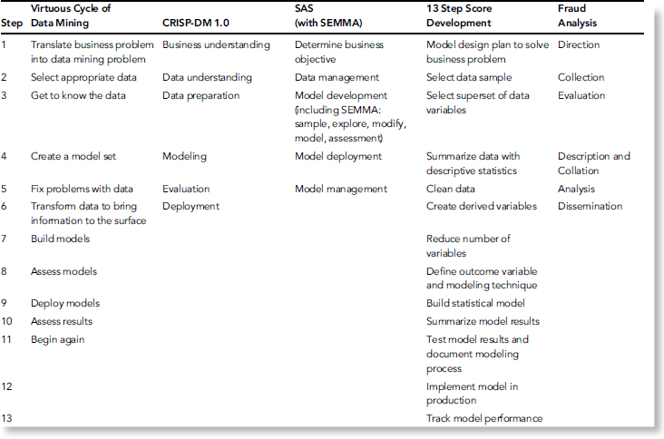
Data analysis has a standard linear process while predictive models have a nonlinear design. This section will compare and contrast three popular predictive modeling methodologies: CRISP-DM 1.0, the SAS (with SEMMA [Sample, Explore, Manipulate, Model and Assess]), and the 13 Step Score Development (shown in Figures 5.1 and Figure 5.2 and Table 5.1). A composite or hybrid of various predictive models will also be identified. Finally, there will be a discussion on how predictive modeling is related to data analysis.

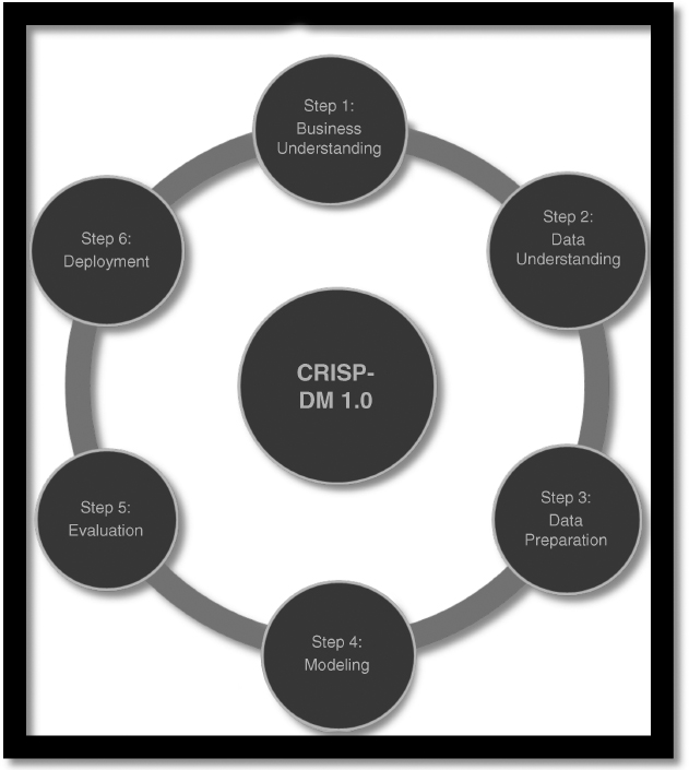
FIGURE 5.1 Cross-Industry Standard Process for Data Mining (CRISP-DM 1.0)

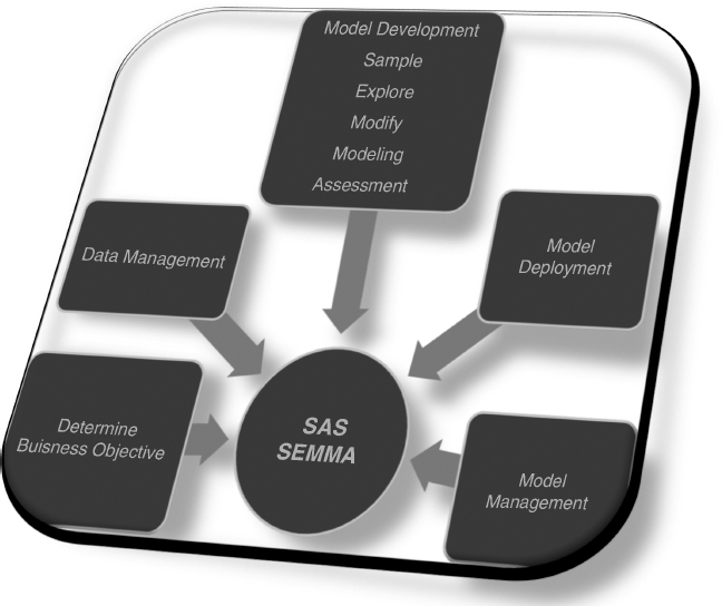
FIGURE 5.2 SAS Model Development Life Cycle (with SEMMA)

COMPARING AND CONTRASTING METHODOLOGIES

When reviewing these models, two things immediately stand out (a difference and a similarity): They have a different number of steps, and each model starts with some type of objective. It is evident that SAS is an incomplete method unless and until it is combined with SEMMA. Furthermore, SAS contains more detailed steps but is simpler when compared to the steps in CRISP-DM, which are very detailed and complex. Another prominent difference is that 13 Scoring uses a scoring strategy throughout the model, whereas neither CRISP-DM nor SAS does. This is probably one of the reasons why there are twice as many steps in the 13 Step Score Development model than in SAS or CRISP-DM.

Step 1 in SAS is to establish a business objective, Step 1 in 13 Step Score Development is to create a model design plan to solve a business problem, and Step 1 in CRISP-DM is to obtain a business understanding. This first stage of 13 Step Score Development and CRISP-DM specifically includes a directive of determining a business/project objective. Understanding the business and objective seems critical to the success of a predictive model. Yet SAS seems to miss much of the detail needed to adequately complete the first step. Both CRISP-DM and 13 Scoring dive into understanding the organization and identifying what resources (including personnel, data, equipment, and facilities) are available throughout the course of the project. These two models take the objective further to design a plan or strategy that outlines a timeline and the tasks that must be completed to achieve success.³

TABLE 5.1 Table of Methodologies by Mock Fraudsters LLC

A surprising difference that occurs at the beginning of these models is the amount of planning and preparation required for the process. SAS keeps Step 1 extremely simple by requiring the modeler merely to determine the type of business decision that needs to be automated and which modeling techniques are appropriate for the problem. Only CRISP-DM takes into account risk and contingency planning. With such a challenging task ahead, it seems unthinkable to proceed without having a backup plan in place. Additionally, for any organization to agree to execute some type of predictive modeling experiment, the executives will want to see a cost-benefit analysis prior to making any decisions; again CRISP-DM is the only model to provide this information.

The next steps of each model correlate to multiple steps in the other models, each involving aspects of the data. For instance, Step 2 of SAS is data management, but Step 3, model development, also includes stages for handling the data. Steps 2 through 7 of 13 Step Score Development all involve the data. Steps 2 and 3 of CRISP-DM play an important role with the data. Obviously, one of the most important parts of predictive modeling is selecting and collecting the data. This task is performed in the second stage of each of these methodologies. Another highly important task involving the data is the act of cleaning it and ensuring it is of high quality. Cleaning data is vital to correct any data entry errors, remove discrepancies from third parties, and eliminate any missing values.⁴

Both SAS and CRISP-DM seem to hold the original data to a higher standard. SAS suggests that the modeler explore the data to find patterns, segments, anomalies, and abnormalities.⁵ During the data understanding phase of CRISP-DM, the modeler is also tasked with exploring the data using querying, visualization and reporting. These two methodologies also take into consideration integrating data from several different sources. Meanwhile, the 13 Step Score Development model places more emphasis on existing variables and creating derived variables. Granted, the other models also utilize derived variables (in the modify phase of SEMMA in SAS and during the construct data phase of Step 3, data preparation, in CRISP-DM). However, these are small pieces of the respective modeling steps. In 13 Step Scoring, the derived variable gets attention in four separate steps: 3, 4, 6, and 7. When it comes to the data, each of these models also allows for the creation, formatting, and substitution of missing values, as long as the modeler can explain why and how those variables were created.

Once the data has been prepared, each methodology moves into a modeling stage. Step 3 of SAS is model development, Step 4 of CRISP-DM is modeling, and Steps 8 and 9 of 13 Step Score Development Model define the outcome variable and the modeling technique, and build the statistical model, respectively. Upon closer examination, the similarities between these “modeling” steps become visible. The first step for each model during this phase is to select the appropriate techniques and tools. Some of the common techniques employed include linear regression, decision trees, neural networks, and traditional statistics. It is not uncommon for a modeler to select several techniques or tools to utilize simultaneously during this period, primarily because not all techniques are suitable for all types of data, especially when various constraints must be taken into consideration.

After the techniques and tools have been chosen, the modeler is ready to build the predictive model. Each of the three methodologies being discussed implements a step to validate or test the model. CRISP-DM seems to duplicate this process by creating a test design of the model to confirm its quality and validity, then requiring an assessment after the model is built. Meanwhile, the other methodologies just experiment with the model in a test environment.

The next phase in the modeling stage is to assess and/or evaluate the model. Again, each of the three methodologies performs some type of an assessment of the model. SAS incorporates this action into Step 3, CRISP-DM places it in both Step 4 and Step 5 (evaluation), and 13 Step Scoring summarizes and documents the process at Steps 10 and 11. During this assessment the modeler may confront new issues that were discovered, such as in SAS; review the qualities of the model, make necessary revisions, and ensure that it meets the stated business objective, such as in CRISP-DM; or summarize the results to determine if the model should even be deployed, as done in 13 Scoring.

If appropriate, the next stage in the process would be to move the model into a live environment. This stage is identified at Step 4, model deployment, of SAS; Step 6, deployment, of CRISP-DM; and Step 12, implement the model in production, of 13 Step Scoring. According to some, deployment can be the most time-consuming stage in predictive modeling. The modeler must create a plan and strategy to deploy the model and ensure that it is operating as expected.⁶

While deployment sounds like the last step, there is still one more piece that completes the methodologies. The final steps are model management, Step 5 of SAS; track model performance, Step 13 of 13 Scoring; and another piece of deployment, Step 6 in CRISP-DM. These concluding steps provide for maintenance of the models, ensuring that they are making the right decisions. A final report may be prepared discussing the results, what went right, or areas that need improvement. In both SAS and CRISP-DM, it seems that if, over the course of time, new data is available or received or new variables identified, the model can be changed or altered to accommodate that data. In fact, with reviews being made in virtually every step of CRISP-DM, the steps could start over at any time. In SAS, the modeler wouldn't go all the way back to the beginning but rather would start over in the second step. This same cyclical process is not apparent in Step 13 or any other step of the 13 Step Score model.

Overall, the SEMMA portion of the SAS model is an easier and faster model to utilize than CRISP-DM. SAS also is more concise and less costly, yet CRISP-DM provides more closure of its processes. While the tasks of each step differ across the three models, they basically cover very similar activities and ultimately strive to accomplish the same goal—predicting future occurrences of a particular incident. The 13 Step Score Development model is a very tedious, time-consuming, and costly model to use. The model will be successful for a few business objectives, like determining the likelihood of a person's debt by viewing monthly expenditures, whether a credit card account will become delinquent, or when it will become delinquent. This depends upon the operational definition and variables chosen earlier in the model. As explained, these models take time to implement. However, since fraud schemes are continuously changing, it is also just as important to begin utilizing the appropriate predictive models quickly.

13 STEP SCORE DEVELOPMENT VERSUS FRAUD ANALYSIS

To better understand the comparison between 13 Step Score Development and Coderre's fraud data analysis, one must first understand the terms employed. For instance, what is a score? A score is a statistically derived formula that applies weights (score points) to new or existing data that provides a prediction, in the form of a single number, about future expected behavior.

In 13 Step Score Development predictive modeling, the initial step is determining the business problem to be solved by the model. Without a clearly defined purpose, any further analysis or model development is a wasted effort. The initial phase sets a course of action or business problem to be solved. In addition, it encompasses setting goals for the projects or tasks at hand; defining milestones and identifying resources (books, reports, people, technology, etc.). Coderre discusses the importance of developing a fraud investigation plan, which serves “as a guide to the investigating team . . . providing a framework for the analysis to be performed.” Within the proposed plan, Coderre notes, “The first step in defining the information required to detect fraud is to identify goals and objectives of the investigation.”⁷ This is akin to defining the business problem, the first step of 13 Step Score Development.

The next step in 13 Step Score Development is selecting a data sample. When selecting the data sample, there must be an initial time frame of study to set a schedule for further examination. This set of data contains the predictor variables—those deemed valuable in determining a probable result. Furthermore, the second or complementary time frame is subsequent though not necessarily immediately after the initial period of study. The second time frame (set of data) would contain the “outcome” variable (i.e., good or bad, true or false, fraud or not fraud). It should be noted that predictive scoring assumes future behavior is similar to prior behavior for comparable events. Another requirement of this phase is to have sufficient data to split into two such groups, one used for model development, the second to be used for validation purposes. The third step, selection of a superset of variables, involves gleaning a manageable and meaningful subset of variables to be employed in the predictive model.

These steps within 13 Step Score Development coincide with Coderre's discussion of overcoming obstacles to obtaining the data. For instance, Coderre mentions that access to data is usually not a technical problem; rather, it is “management's or the client's reluctance to provide access to the application.”⁸ Furthermore, Coderre devotes a significant amount of time in his text to the importance of incorporating computer-assisted audit tools and techniques (CAATTs); he notes: “CAATTs have the ability to improve the range and quality of audit and fraud investigation results.”⁹ CAATTs are more than tools to enhance the collection of data. They can aid in the evaluation, collation, and description of the data.

The fourth step of 13 Step Score Development is summarization, where each variable is summarized using descriptive statistics (e.g., mean, median, mode, minimum, maximum, variance, etc.). Coderre mirrors this step by encapsulating three different analytical techniques: summarization, stratification, and cross-tabulation/pivot tables, under the main heading of performing an overview of the data. Though the aforementioned analyses speak to a much broader examination than simple statistical analysis, they do possess components referenced in the 13 Step Score Development methodology.

Cleaning the data, 13 Step Score Development's fifth step, involves plugging in appropriate values for variables that do not possess them; determining the range of variables; and correcting illogical/impossible values of variables (e.g., Age = 1948). The next step involves the creation of derived variables. Derived variables are indicative of a possible relationship between two or more variables. For instance, if employees with little time on the job (TOJ) and/or who are on the lower end of the pay scale are responsible for a greater percentage of fraud within a business, then a derived variable would combine the time on the job with the number of raises (or aggregate value of growth in pay) an employee received. This derived variable could be indicative of a fraudster.

A prime example would be the following:

CRISP-DM VERSUS FRAUD DATA ANALYSIS

There are many similarities and differences between CRISP-DM predictive modeling methodology and fraud data analysis. Each has many stages in common and both methods are flexible and iterative.

To begin with, CRISP-DM was developed to utilize data mining techniques to deliver value to the large amounts of data kept by most organizations. Fraud data analysis utilizes data mining techniques to analyze large amounts of information looking for red flags that could be indicative of fraudulent behavior or inefficiencies in the organization's processes.

Both methods begin with an objective or goal they attained via different methodologies. In CRISP-DM, this is conducted in the business understanding phase; in fraud data analysis, it is normally determined by an assessment of a risk factor, a standard audit process, a tip of wrongdoing, or another form of predicate act.¹⁰

The next phase in CRISP-DM is data understanding. In this phase, many data mining techniques, such as collecting the requisite data, are used. The data will be analyzed using a variety of techniques. Coderre describes how fraud data analysis uses summarization, gaps, duplicates, stratification, join/relate, aging, and many other methods to evaluate the data to find, among other things, outliers and anomalies, trends and patterns. During this phase, both methods examine the data quality, asking: Does the data have similar meanings or values? Are there deviations in the data? Are these noted deviations simply noise, or are they pertinent to the evaluation process?

The third phase in CRISP-DM is data preparation. This phase takes the previous activities completed in data understanding and reevaluates them. It asks if the data is relevant to the project: For example, is the data collected enough, or do we need additional data? When the quality of the data was verified in the previous step, did this eliminate data sets or values within the data? Are new data sets required? Can values be retrieved from other sources? How necessary are these values or attributes to our objective? In this phase, both methods continue to use data mining techniques to integrate the data and to store and evaluate the results. These types of questions and concerns are also weighed when conducting fraud data analysis. It is essential in both methods to continually reevaluate the data as well as any derived variables to ensure their relevance, integrity, and accuracy.

Modeling is the fourth phase in CRISP-DM. This is the phase where modeling techniques such as decision trees, neural nets, or logistic regression are employed. CRISP-DM's main focus is to predict the likelihood that the outcome of the model is or is not fraud. This enables CRISP-DM to be used as a tool in real-time scenarios. CRISP-DM tests its model in this phase to decide if further analysis is needed: new data retrieved, larger samples examined, drilling-down methods implemented. At this stage, fraud data analysis may come to an end if it has not identified any wrongdoing or irregularities; however, if anomalies or red flags indicating a potential fraud problem are discovered, fraud data analysis evaluates whether additional information/evidence is needed (e.g., different data sets, larger samples sizes, etc.).

The fifth phase in CRISP-DM is evaluation. In the modeling phase, CRISP-DM evaluated its data mining activities, but in the evaluation process, it determines whether it met its business objective or not. Although fraud data analysis performs an evaluation as well, this is akin to CRISP-DM's modeling phase.

The last phase in CRISP-DM is the deployment stage. CRISP-DM assesses its strategy on how to implement its model, get it to end users, and integrate it within the organization's systems. Fraud data analysis, in contrast, may deploy a “script” that would have been created if it found red flags: possible indicators of malfeasance. This measure would be completed in the same step as the CRISP-DM modeling phase. These scripts can be deployed to detect fraud in its early stages and/or act as a deterrent to prevent future fraud.

In both methods, reports are generated to track the process, its success and failures, and the rationale for choosing one direction over another, as well as the elimination or inclusion of data, and so on. It is imperative in both methods that the end results are effectively communicated to senior management and all appropriate personnel. It is only with effective communication and thorough documentation of the analysis and results that an organization may make insightful and informed decisions.

SAS/SEMMA VERSUS FRAUD DATA ANALYSIS

SAS, a developer of predictive analytic software, has created a best practice of predictive modeling. This methodology is called SEMMA. SEMMA is an acronym for sample, explore, manipulate, model, and assess. In both SEMMA and fraud data analysis, the process begins when a problem is identified or a business objective is determined. The business objective for fraud data analysis could be to determine if fraudulent or “ghost” employees are on the payroll. The objective for SEMMA would be to determine which employees on the payroll have the highest likelihood of being ghost employees.

The primary difference between SEMMA and fraud data analysis is that SEMMA is forward-looking or predictive. SEMMA and other predictive modeling techniques try to anticipate when a transaction is fraudulent, warranting further investigation. For predictive modeling, quick identification of fraud is imperative. For example, the sooner you determine that a credit card number has been stolen, the sooner you can deactivate the card and thus minimize losses.

Fraud analytics uses historical information to determine if a fraudulent act has occurred. Timing is not as crucial here, because the goal of fraud analytics is to determine if a fraudulent act occurred and who is responsible rather than the immediate prevention of future acts.

SEMMA uses data mining, which SAS defines as “the process of selecting, exploring and modeling large amounts of data to uncover previous unknown patterns of data for business advantage.” Since many sources of data today are extremely large and would take many hours to review, SEMMA begins by sampling a subset of the data. Sampling the data reduces the amount of time to process these initial attempts. This is different from fraud data analysis whereby, with the use of CAATTs, all the data can be included in the population and reviewed. A sample of data is not required.

The second step of SEMMA is exploration. This is the step where the user becomes familiar with the data. This is similar to the step in fraud data analysis called understanding the data. In fraud data analysis and SEMMA, this step could include looking for gaps, reasonableness, completeness, and period-over-period comparisons.

The third step of SEMMA is modification. This is the step where the user can modify or manipulate the data. One example of modification may be to place the data into buckets based on stratification. In fraud data analysis, there is not a true equivalent to this stage, but the user may want to modify the data based on syntax (remove commas, reduce length of characters).

The fourth step of SEMMA is modeling. This is where predictive modeling and fraud data analysis begin to differ significantly. In SEMMA, patterns in the data are analyzed and the question is raised: What causes these patterns? During this stage, a hypothesis would be created and tested. This step includes creating scores based on the patterns in the data. There is no equivalent to this stage in fraud analytics since its goal is to determine what happened, not to predict future events.¹¹

The final step in SEMMA is assessment. This is the step where the user reviews the results of the model and determines whether it is accurately predicting fraudulent behavior. This is also when the model would be modified or data selection changed to ensure the most accurate model and score. Fraud analytics may deploy a script at this stage that can be run on recurring data sets. The scripts depend on the user periodically reviewing and updating them as necessary.

Now that the individual predictive modeling methodologies have been compared and contrasted to fraud analytics, we will discuss the similarities and differences among the three predictive models. This section is divided into seven main categories: business understanding/problem definition, data collection/assessment, data preparation, variable establishment, model selection, model deployment, and model evaluation/validation.

CONFLICTS WITHIN METHODOLOGIES

While many predictive models have their own flow and level of detail, occasionally pieces may stick out or seem unusual to another modeler. For example, according to the SAS Institute, the second stage, data management, “is the phase of the model development life cycle that generally lacks appropriate rigor.” Yet when studying the overall model, it appears evident that the model focuses more on the third stage, model development. It is at this point that SEMMA is introduced and the modeling process is truly developed. To avoid this contradiction, should sampling, exploration, and maybe even the modification stages be more appropriately included in the data management stage rather than the model development stage.¹²

Other conflicts may appear in CRISP-DM during the first and second steps, business understanding and data understanding, respectively. During the first stage the modeler is tasked with determining data mining goals, including defining “the criteria for a successful outcome to the project.” Yet at the second stage, the modeler finally gets an opportunity to understand the data available and/or collected. It seems necessary to have that knowledge before writing a valid goal. Another task in the first stage is to create a project plan; and as previously discussed, predictive modeling is nonlinear. It is obvious that following a step-by-step plan is contradictory to a nonlinear design.¹³

From the information reviewed in 13 Step Scoring, it is difficult to conclude whether conflicts exist or the model is supposed to be as redundant as it appears. For instance, Step 9, build the statistical model, and Step 11, test model results and document modeling process, both include the task of testing the score results with original data analysis. Other steps that have a similar duplication are Steps 11 and Step 12, implement the model in production; both of these steps include track model performance in production to ensure it works as expected. Step 13 is track model performance. A modeler would likely be confused as to when these tasks should be completed or will question why they are recurring. Buried behind the repetitiveness of the model, there is a blatant contradiction between Steps 6 and 7. In Step 6, the modeler should be creating derived variables; meanwhile, in Step 7, the modeler is encouraged to reduce the number of variables by selecting a superset of the data variables, combining categorical variables, or restricting the range of outliers. It seems unlikely that a modeler would put forth the effort to create variables and later eliminate them.

COMPOSITE METHODOLOGY

With a plethora of different options pertaining to the order of the phases, what items need additional focus, and which techniques to use, it's not surprising that an abundance of predictive models exist. Without a doubt, some are better than others, but none can be perfect all of the time. Borrowing steps from several predictive analytic models that are used today, I have created a hybrid predictive analytic model. Table 5.1 depicts a high-level overview of the steps contained in the various models. Table 5.2 is overview of comparisons between Fraud Analytics and Predictive Analytics.

TABLE 5.2 Fraud Analytics in Comparison to Predictive Analytics (Modeling)

Fraud Analytics	Predictive Analytics (Modeling)
Uses historical data to detect fraud that has already occurred	Uses historical data to predict future outcomes
Linear process; the steps are performed in order, and typically the process is not repeated	Nonlinear process; steps can be skipped, and the process is reiterative
A hypothesis is formed at the beginning of the fraud engagement	Models are defined and created based on the particular business process
Analysis stage may continue longer than expected if additional hypotheses are formed	Process is repeated if new data or different variables are discovered
Hypothesis is tested and amended as necessary	Models are tested to determine success; modifications are made as necessary
Fraud analysis is used to locate fraud and can provide a model for future detection	Predictive modeling is used to complement the fraud analysis by creating a process to show red flags
Data quality is important to the analyst's ability to discover the fraud	Data quality is important to the success of the model
Uses all available data	Uses a sample of the available data
Constructs data (mean, median, mode) for statistical analysis purposes	Constructs data to fill in missing variables
Fraud analysis is performed as needed, not on a regular recurring basis, and ends with a final conclusion	Models are repetitive and cyclical in nature; they are always in process
Looks for anomalies in the data	Looks for anomalies in the data
Outcome cannot be predicted and is known only after the dissemination stage	Outcome or final goal must be specifically defined

The following are the specific steps used by fraud examiners:

• Identify the business problem and objective. Define the problem, identify goals and phases, business requirements, and include any predictions.
• Data sampling and understanding. Collect, describe, and understand the data. Identify time frame for collecting data. Decipher types of data, how much is needed, and if it is balanced.
• Data management. Evaluate, clean, prepare, and select data. Fix problems identified, add or create variables, format data, perform in-depth data analysis, validation, modification, and exploration.
• Modeling. Create the model. Then model management and deployment of model. Build models, such as multiple, linear, or logistical regression, decision trees, neural networks, and link analysis. Deploy the model, select model technique appropriate for each specific problem, monitor, and maintain the model. Calculate points, translation, code compilation, operational platform reports, and data distribution, to validate the model.
• Evaluation and analysis. Perform overall assessment. Identify false negatives and false positives. Track model performance, cost-benefit analysis, and fraud loss reductions versus loss of investigative impacts. Perform a review process to determine next steps, locate deficiencies, and clarify future updates. Confirm that all the questions have been answered.
• Dissemination. Deliver results to all interested parties.
• Begin again. Review the process, establish next steps. Report if a modeler detected any unexpected facts that were learned during the process. Identify what data would be desired for future tests. Determine if the same or new techniques should be used. Track model performance; use fraud detection charts. Ascertain whether a real-time score is generated. Conclude by deciding if the results can be replicated in every model test and if there are any new questions to answer.

COMPARING AND CONTRASTING PREDICTIVE MODELING AND DATA ANALYSIS

While there are certainly similarities between data analysis and predictive modeling, there are also significant differences. To design a predictive model, one must understand the data and the fraud. Data analysis looks at historic data to determine where and how a fraud occurred or is occurring, while predictive modeling uses historic data to predict the possibility of future fraud incidents. These steps use historical data differently, ultimately implying they are complementary to each other, creating one continuous cycle. Some may even suggest that predictive modeling is the next natural step following a fraud analysis engagement.

As in predictive analysis (modeling), there are specific steps to be followed in the fraud data analysis process. However, unlike the nonlinear design of modeling, data analysis is generally performed in a systematic order, and the steps typically are not repeated for the duration of the engagement, except to verify calculations. Additionally, all of the steps are completed, whereas modeling provides the option to skip or not utilize steps (see Table 5.2).

The fraud analysis process can be summarized in six steps:

1. Direction. Decipher the raw data to determine where you want to go with the analysis.
2. Collection. Determine a plan for how the data will be collected and begin the process.
3. Evaluation. Devise a strategy for how you will work with the data. Formulate a plan for how the red flags will be discovered.
4. Collation and description. Put data in an easily understood format. Describe the data, including any missing information. During this step one or more hypotheses may be developed.
5. Analysis. Work with the data and test the hypotheses. Make amendments as necessary.
6. Dissemination. Distribute results of analysis to the appropriate parties. Use caution when deciding who needs the information.

The direction stage of data analysis can easily be compared to the business objective phases of the predictive modeling methodologies. It is at this phase where an auditor or investigator will want to determine a goal. There is a greater emphasis on the planned outcome: solving the fraud problem with analysis versus solving a business problem. The collection stage equates to the various data collection steps in predictive modeling. The fraud examiner will gather all the available data, whereas modeling gathers only a sampling of the data to be used. In the third step, the fraud examiner will begin evaluating the data: getting a better understanding of the data characteristics, confirming the reliability of the source, and possibly identifying trends. As previously discussed, data quality needs special attention because it can make or break the success of a predictive model. Likewise fraud analysis reviews data quality at practically every step of the process. Without quality data, it is unlikely that an analyst will achieve the desired goal during the engagement.

During the fourth step, collate and describe, the investigator really begins to get to know the data. The investigator performs a quick overview in order to summarize and sort the data. It is also common for the fraud examiner to convert the data into an easily understood format, such as graphs and charts.¹⁴ No step in predictive analysis (modeling) entirely correlates to the data collation phase of fraud analysis. In the interim, a fraud examiner may even construct data. Keep in mind that when a modeler constructs data, it is to fill in missing variables; when an auditor or investigator constructs data, it is for statistical analysis purposes (i.e., mean, median, mode, etc.). By performing these steps, the auditor or investigator will be able to formulate one or more hypotheses about the data and the type of fraud that has been committed.

Then the most intense phase of the process begins—the analysis. This step is used to review the data in order to identify anomalies and discrepancies that require additional testing or investigation. This could be compared to the testing or deployment stages of the predictive models since the investigator in essence is testing the hypotheses. As when refining predictive models, an investigator's hypothesis may change during the analysis phase. For example, at the outset the auditor may suspect an overbilling scheme, but through the course of the analysis it becomes apparent that it is a duplicate billing scheme. Yet just because the hypothesis is altered does not mean the process starts over. There is no need to begin the fraud analysis process again.

The last step in the fraud analysis process is dissemination. This is similar to the last stage in predictive analytics (modeling), in that it provides a report and the results of the analysis. But it is also substantially different since the last step in fraud analysis is final. No monitoring or ongoing maintenance takes place, as occurs with predictive models. Another difference here is with what a client would expect from either of these processes. With a predictive model, there is some predefined anticipated outcome, whereas fraud analysis cannot predict the results at the beginning of the engagement. The conclusions of fraud analysis are learned and understood only after the dissemination stage.

Clearly the most important part of fraud analysis and predictive modeling is the data. Data must be acquired, understood, sorted, analyzed, manipulated, and linked to make final assessments. Some of the most common techniques used in fraud detection analysis include but are not limited to: aging, join/relation, summarizations, stratification, cross tabulation, trend analysis, regression analysis, and parallel simulation. The ultimate goal of these techniques is to gain a better understanding of the data.

In fraud analysis, the fraud examiner uses these techniques during the collation stage, since focusing on the data becomes the examiner's biggest responsibility. Likewise, in a fraud examiners' composite model, it may behoove the modeler to perform these techniques in the data management phase. When utilizing these methods in a predictive model, the modeler will be able to delete the outliers, restrict the range of values, and correct errors. This knowledge will allow the modeler to consider the imperfections of the data prior to building a model. A difference arises when trend or regression analysis or parallel simulation is performed. While it would be expected that an investigator would utilize these techniques during Step 5, analysis, these techniques may be performed in the third step of the composite—data management—or during the modeling and evaluation stages. This difference is simply because these techniques are significantly more complicated than the others and require more effort.

The similarity between predictive modeling and data analysis is that the auditors and investigators are able to interact freely with the data. While the end result of analysis and the types of analyses performed may differ greatly, the volume of data being analyzed is large and requires the use of CAATTs (i.e., ACL Analytics, CaseWare IDEA, and Microsoft Excel). In addition to the use of CAATTs, it is also necessary for a fraud examiner, analyst, auditor, or investigator to perform the proper analysis. The human component is needed to determine what to look for where the computer component provides the how. Fraud analysis cannot be performed without both human and mechanical parts. While the mechanical part is far more efficient, human logic is the only way to reevaluate testing and determine changes in a continuous, iterative process.¹⁵ Furthermore, as accounting systems become more dependent on electronic resources and less dependent on paper, the trail to follow is no longer tangible pieces of paper but as digital code. Due to the increase in digital information, fraud examiners, analysts, auditors, and investigators must be prepared to move in the same direction.¹⁶

The predictive analysis model created by the fraud examiner utilizes the most useful and beneficial steps from the other predictive models and fraud analysis. The composite is an ideal example of a well-rounded and comprehensive model. Similar to fraud analysis, the composite was designed to provide information to business management by outlining areas of potential fraud and weaknesses that should be addressed for the security of the organization. Granted, it is not perfect, but it allows fraud examiners to learn from the experience. The final report also provides closure and recommendations to the possible victim of fraud.

Based on this study of several predictive models, it is evident that not all models are created equal. Moreover, some techniques are more likely to achieve goals and determine solutions when taking into consideration the problem and available data. Although every circumstance is different and techniques change based on the situation, certain techniques are not used frequently enough. With that information in mind, I have created a better predictive analytics composite model which incorporates several techniques that are necessary and successful in multiple instances.

NOTES

1. David Coderre, Fraud Detection: A Revealing Look at Fraud, 2nded. (N.P.: Ekaros Analytical, 2004), p. 14.

2. Delena D. Spann and Wesley Wilhelm, “Advanced Fraud Analysis” (ECM 642), presented by professors at Utica College, 2008.

3. P. Chapman, J. Clinton, R. Kerber, T. Khabaza, T. Reinartz, C. Shearer, and R. Worth, “CRISP DM 1.0, Step-by-Step Data Mining,” CRISP Consortium, 2008.

4. J. Livermore and R. Betancourt, “Operationalizing Analytic Intelligence: A Solution for Effective Strategies in Model Deployment,” SAS Institute, 2005.

5. Ibid.

6. Livermore and Betancourt, “Operationalizing Analytic Intelligence.”

7. Coderre, Fraud Detection., p. 14.

8. Ibid. p. 51.

9. David Coderre, Fraud Analysis Techniques Using ACL (Hoboken, NJ: John Wiley & Sons, 2009).

10. Step by Step Data Mining Guide, SPSS, Inc., 2000. ftp://ftp.software.ibm.com/software/analytics/spss/support/Modeler/Documentation/14/UserManual/CRISP-DM.pdf

11. SAS Institute, “From Data to Business Advantage: Data Mining, The SEMMA Methodology and SAS Software,” white paper, 1998, http://old.cba.ua.edu/~mhardin/DM_INS.pdf.

12. Livermore and Betancourt, “Operationalizing Analytic Intelligence.”

13. Chapman et al., “CRISP-DM 1.0.”

14. Ibid.

15. Coderre, Fraud Detection.

16. Ibid.