Chapter 23

Global Illumination

Many surfaces in the real world receive most or all of their incident light from other reflective surfaces. This is often called indirect lighting or mutual illumination. For example, the ceilings of most rooms receive little or no illumination directly from luminaires (light-emitting objects). The direct and indirect components of illumination are shown in Figure 23.1.

Although accounting for the interreflection of light between surfaces is straightforward, it is potentially costly because all surfaces may reflect any given surface, resulting in as many as O(N2) interactions for N surfaces. Because the entire global database of objects may illuminate any given object, accounting for indirect illumination is often called the global illumination problem.

There is a rich and complex literature on solving the global illumination problem (e.g., Appel, 1968; Goral, Torrance, Greenberg, & Battaile, 1984; Cook et al., 1984; Immel et al., 1986; Kajiya, 1986; Malley, 1988). In this chapter, we discuss two algorithms as examples: particle tracing and path tracing. The first is useful for walkthrough applications such as maze games, and as a component of batch rendering. The second is useful for realistic batch rendering. Then we discuss separating out “direct” lighting where light takes exactly once bounce between luminaire and camera.

23.1 Particle Tracing for Lambertian Scenes

Recall the transport equation from Section 18.2:

$L_s\left(k_o\right)={\displaystyle {\int }_{\text{all}{k}_i}\rho \left(k_i,k_o\right)}{L}_f\left(k_i\right)\cos {\theta }_{i}d{\sigma }_i.$

The geometry for this equation is shown in Figure 23.2. When the illuminated point is Lambertian, this equation reduces to:

$L_s=\frac{R}{\pi }{\displaystyle {\int }_{\text{all}{k}_i}{L}_f\left(k_i\right)}\cos {\theta }_{i}d{\sigma }_i,$

where R is the diffuse reflectance. One way to approximate the solution to this equation is to use finite element methods. First, we break the scene into N surfaces each with unknown surface radiance Li, reflectance Ri, and emitted radiance Ei. This results in the set of N simultaneous linear equations

$L_i=E_i+\frac{R_i}{\pi }{\displaystyle \sum _{j=1}^n{k}_{ij}{L}_j,}$

where kij is a constant related to the original integral representation. We then solve this set of linear equations, and we can render N constant-colored polygons. This finite element approach is often called radiosity.

An alternative method to radiosity is to use a statistical simulation approach by randomly following light “particles” from the luminaire through the environment. This is a type of particle tracing. There are many algorithms that use some form of particle tracing; we will discuss a form of particle tracing that deposits light in the textures on triangles. First, we review some basic radiometric relations. The radiance L of a Lambertian surface with area A is directly proportional to the incident power per unit area:

$L=\frac{\Phi }{\pi A},\text{ (23.1)}$

where Φ is the outgoing power from the surface. Note that in this discussion, all radiometric quantities are either spectral or RGB, depending on the implementation. If the surface has emitted power Φe, incident power Φi, and reflectance R, then this equation becomes

$L=\frac{{\Phi }_e+R{\Phi }_i}{\pi A}.$

If we are given a model with Φe and R specified for each triangle, we can proceed luminaire by luminaire, firing power in the form of particles from each luminaire. We associate a texture map with each triangle to store accumulated radiance, with all texels initialized to

$L=\frac{{\Phi }_e}{\pi A}.$

If a given triangle has area A and nt texels, and it is hit by a particle carrying power ϕ, then the radiance of that texel is incremented by

$\Delta L=\frac{n_t\varphi }{\pi A}.$

Once a particle hits a surface, we increment the radiance of the texel it hits, probabilistically decide whether to reflect the particle, and if we reflect it we choose a direction and adjust its power.

Note that we want the particle to terminate at some point. For each surface we can assign a reflection probability p to each surface interaction. A natural choice would be to let p = R as it is with light in nature. The particle would then scatter around the environment, not losing or gaining any energy until it is absorbed. This approach works well when the particles carry a single wavelength (Walter, Hubbard, Shirley, & Greenberg, 1997). However, when a spectrum or RGB triple is carried by the ray as is often implemented (Jensen, 2001), there is no single R and some compromise for the value of p should be chosen. The power ϕ′ for reflected particles should be adjusted to account for the possible extinction of the particles:

${\varphi }^{\prime }=\frac{R\varphi }{p}.$

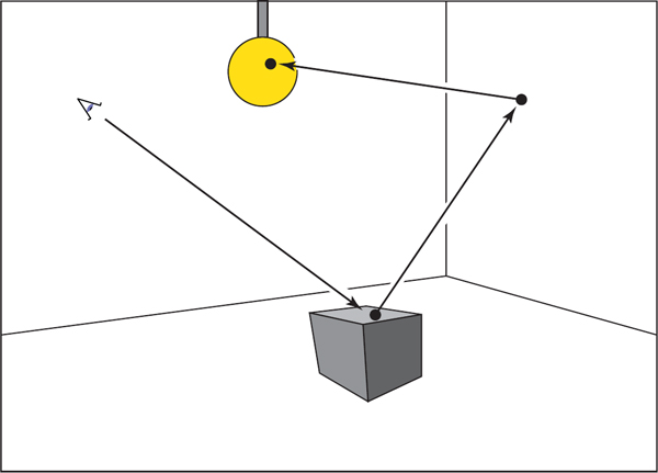
Note that p can be set to any positive constant less than one, and that this constant can be different for each interaction. When p > R for a given wavelength, the particle will gain power at that wavelength, and when p < R it will lose power at that wavelength. The case where it gains power will not interfere with convergence because the particle will stop scattering and be terminated at some point as long as p < 1. For the remainder of this discussion we set p = 0.5. The path of a single particle in such a system is shown in Figure 23.3.

A key part to this algorithm is that we scatter the light with an appropriate distribution for Lambertian surfaces. As discussed in Section 14.4.1, we can find a vector with a cosine (Lambertian) distribution by transforming two canonical random numbers (ξ1, ξ2) as follows:

$a=\left(\cos \left(2\pi {\xi }_1\right)\sqrt{{\xi }_2,}\sin \left(2\pi {\xi }_1\right)\sqrt{{\xi }_2,}\sqrt{1-\xi 2}\right).\text{ (23.2)}$

Note that this assumes the normal vector is parallel to the z-axis. For a triangle, we must establish an orthonormal basis with w parallel to the normal vector. We can accomplish this as follows:

$\begin{array}{cc}\hfill w& =\frac{n}{||n||},\hfill \\ \hfill u& =\frac{p_1-p_0}{||p_1-p_0||},\hfill \\ \hfill v& =w\times u,\hfill \end{array}$

where pi are the vertices of the triangle. Then, by definition, our vector in the appropriate coordinates is

$\mathbf{\text{a}}=\cos \left(2\pi {\xi }_1\right)\sqrt{{\xi }_2\mathbf{u}}+\sin \left(2\pi {\xi }_1\right)\sqrt{{\xi }_{2}v}+\sqrt{1-{\xi }_2\mathbf{w}}.\text{ (23.3)}$

In pseudocode our algorithm for p = 0.5 and one luminaire is:

for (Each of n particles) do

 RGB phi = Φ/n

 compute uniform random point a on luminaire

 compute random direction b with cosine density

 done = false

 while not done do

 if (ray a + tb hits at some point c) then

  add ntRϕ/(πA) to appropriate texel

  if (ξ1 > 0.5) then

   ϕ = 2Rϕ

   a = c

   b = random direction with cosine density

 else

  done = true

Here ξi are canonical random numbers. Once this code has run, the texture maps store the radiance of each triangle and can be rendered directly for any viewpoint with no additional computation.

23.2 Path Tracing

While particle tracing is well suited to precomputation of the radiances of diffuse scenes, it is problematic for creating images of scenes with general BRDFs or scenes that contain many objects. The most straightforward way to create images of such scenes is to use path tracing (Kajiya, 1986). This is a probabilistic method that sends rays from the eye and traces them back to the light. Often path tracing is used only to compute the indirect lighting. Here we will present it in a way that captures all lighting, which can be inefficient. This is sometimes called brute force path tracing. In Section 23.3, more efficient techniques for direct lighting can be added.

In path tracing, we start with the full transport equation:

$L_s\left(k_o\right)=L_e\left(k_o\right)+{\displaystyle {\int }_{\mathrm{all}{k}_i}\rho \left(k_i,k_o\right)}Lf\left(k_i\right)\cos {\theta }_{i}d{\sigma }_i.$

We use Monte Carlo integration to approximate the solution to this equation for each viewing ray. Recall from Section 14.3, that we can use random samples to approximate an integral:

${\displaystyle {\int }_{x\in S}g}\left(x\right)d\mu \approx \frac{1}{N}{\displaystyle \sum _{i=1}^N\frac{g\left(x_i\right)}{p\left(x_i\right)}},$

where the xi are random points with probability density function p. If we apply this directly to the transport equation with N = 1 we get

$L_s\left(k_o\right)\approx L_e\left(k_o\right)+\frac{\rho \left(k_i,k_o\right)L_f\left(k_i\right)\cos {\theta }_{i}d{\sigma }_i}{p\left(k_i\right)}.$

So, if we have a way to select random directions ki with a known density p, we can get an estimate. The catch is that Lf (ki) is itself an unknown. Fortunately, we can apply recursion and use a statistical estimate for Lf (ki) by sending a ray in that direction to find the surface seen in that direction. We end when we hit a luminaire and Le is nonzero (Figure 23.4). This method assumes lights have zero reflectance, or we would continue to recurse.

In the case of a Lambertian BRDF (ρ = R/π), we can use a cosine density function:

$p\left(k_i\right)=\frac{\cos {\theta }_i}{\pi }.$

A direction with this density can be chosen according to Equation (23.3). This allows some cancellation of cosine terms in our estimate:

$L_s\left(k_o\right)\approx L_e\left(k_o\right)+R{L}_f\left(k_i\right).$

In pseudocode, such a path tracer for Lambertian surfaces would operate just like the ray tracers described in Chapter 4, but the raycolor function would be modified:

RGB raycolor(ray a + tb, int depth)

if (ray hits at some point c) then

 RGB c = Le(‒b)

 if (depth < maxdepth) then

 compute random direction d

 return c + R raycolor(c + sd, depth+1)

 else

 return background color

This will result in a very noisy image unless either large luminaires or very large numbers of samples are used. Note the color of the luminaires must be well above one (sometimes thousands or tens of thousands) to make the surfaces have final colors near one, because only those rays that hit a luminaire by chance will make a contribution, and most rays will contribute only a color near zero. To generate the random direction d, we use the same technique as we do in particle tracing (see Equation (23.2)).

In the general case, we might want to use spectral colors or use a more general BRDF. In practice, we should have the material class contain member functions to compute a random direction as well as compute the p associated with that direction. This way materials can be added transparently to an implementation.

23.3 Accurate Direct Lighting

This section presents a more physically based method of direct lighting than Chapter 10. These methods will be useful in making global illumination algorithms more efficient. The key idea is to send shadow rays to the luminaires as described in Chapter 4, but to do so with careful bookkeeping based on the transport equation from the previous chapter. The global illumination algorithms can be adjusted to make sure they compute the direct component exactly once. For example, in particle tracing, particles coming directly from the luminaire would not be logged, so the particles would only encode indirect lighting. This makes nice looking shadows much more efficiently than computing direct lighting in the context of global illumination.

23.3.1 Mathematical Framework

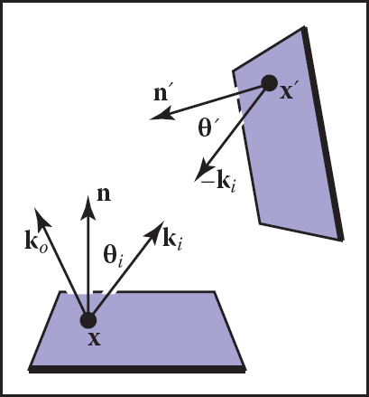
To calculate the direct light from one luminaire (light emitting object) onto a non-emitting surface, we solve a form of the transport equation from Section 18.2:

$L_s\left({x,k}_o\right)={\displaystyle {\int }_{\mathrm{all}{\mathbf{\text{x}}}^{\prime }}\frac{\rho \left({\mathbf{k}}_i,{\mathbf{k}}_o\right)L_e\left({\mathbf{\text{x}}}^{\prime },-{\mathbf{k}}_i\right)v\left(\mathbf{x},{\mathbf{\text{x}}}^{\prime }\right)\cos {\theta }_i\cos {\theta }^{\prime }}{{||\mathbf{x}-{\mathbf{\text{x}}}^{\prime }||}^2}}d{A}^{\prime }.\text{ (23.4)}$

Recall that Le is the emitted radiance of the source, v is a visibility function that is equal to 1 if x “sees” x′ and zero otherwise, and the other variables are as illustrated in Figure 23.5.

If we are to sample Equation (23.4) using Monte Carlo integration, we need to pick a random point x′ on the surface of the luminaire with density function p (so x′ ~ p). Just plugging into Equation (14.5) with one sample yields

$L_s\left({x,k}_o\right)\approx \frac{\rho \left(k_i,k_0\right)L_e\left({\mathbf{\text{x}}}^{\prime },-{\mathbf{k}}_i\right)v\left(\mathbf{x},{\mathbf{\text{x}}}^{\prime }\right)\cos {\theta }_i\cos {\theta }^{\prime }}{p\left({\mathbf{\text{x}}}^{\prime }\right){||\mathbf{x}-{\mathbf{\text{x}}}^{\prime }||}^2}.\text{ (23.5)}$

If we pick a uniform random point on the luminaire, then p = 1/A, where A is the area of the luminaire. This gives

$L_s\left({\mathbf{x},\mathbf{k}}_o\right)\approx \frac{\rho \left({\mathbf{k}}_i,{\mathbf{k}}_0\right)L_e\left({\mathbf{\text{x}}}^{\prime },-{\mathbf{k}}_i\right)v\left(\mathbf{x},{\mathbf{\text{x}}}^{\prime }\right)A\cos {\theta }_i\cos {\theta }^{\prime }}{{||\mathbf{x}-{\mathbf{\text{x}}}^{\prime }||}^2}.\text{ (23.6)}$

We can use Equation (23.6) to sample planar (e.g., rectangular) luminaires in a straightforward fashion. We simply pick a random point on each luminaire.

The code for one luminaire is:

color directLight(x, ko, n)

pick random point x′ with normal vector n′ on light

d = x′ − x

ki = d/∥d∥

if (ray x + td has no hits for t < 1 ‒ ∈) then

 return ρ(ki, ko)Le(x′, ‒ ki)(n · d)(‒n′ · d)/∥d∥4

else

 return 0

The above code needs some extra tests such as clamping the cosines to zero if they are negative. Note that the term ∥d∥4 comes from the distance squared term and the two cosines, e.g., n · d = ∥d∥ cos θ because d is not necessarily a unit vector.

Several examples of soft shadows are shown in Figure 23.6.

23.3.2 Sampling a Spherical Luminaire

Though a sphere with center c and radius R can be sampled using Equation (23.6), this sampling will yield a very noisy image because many samples will be on the back of the sphere, and the cos θ′ term varies so much. Instead, we can use a more complex p(x′) to reduce noise.

The first nonuniform density we might try is p(x′) ∝ cos θ′. This turns out to be just as complicated as sampling with p(x′) ∝ cos θ′ ∥x′ — x∥2, so we instead discuss that here. We observe that sampling on the luminaire this way is the same as using a constant density function q(ki) = const defined in the space of directions subtended by the luminaire as seen from x. We now use a coordinate system defined with x at the origin, and a right-handed orthonormal basis with w = (c — x)/∥c − x∥, and v = (w × n)/∥(w × n)∥ (see Figure 23.7). We also define (α, ϕ) to be the azimuthal and polar angles with respect to the uvw coordinate system.

The maximum α that includes the spherical luminaire is given by

${\alpha }_{\max }=\arcsin \left(\frac{R}{||x-c||}\right)=\arccos \sqrt{1-{\left(\frac{R}{||x-c||}\right)}^2.}$

Thus, a uniform density (with respect to solid angle) within the cone of directions subtended by the sphere is just the reciprocal of the solid angle 2π(1 — cos αmax) subtended by the sphere:

$q\left(k_i\right)=\frac{1}{2\pi \left(1-\sqrt{1-{\left(\frac{R}{||x-c||}\right)}^2}\right)}.$

And we get

$\left[\begin{array}{c}\cos \alpha \\ \varphi \end{array}\right]=\left[1-{\xi }_1+{\xi }_1\begin{array}{l}\sqrt{1-{\left(\frac{R}{||x-c||}\right)}^2}\hfill \\ 2\pi {\xi }_2\hfill \end{array}\right].$

This gives us the direction ki. To find the actual point, we need to find the first point on the sphere in that direction. The ray in that direction is just (x + tki), where ki is given by

$k_i=\left[\begin{array}{ccc}{u}_x& v_x& w_x\\ u_y& v_y& w_y\\ u_z& v_z& w_z\end{array}\right]\left[\begin{array}{c}\cos \varphi \sin \alpha \\ \sin \varphi \sin \alpha \\ \cos \alpha \end{array}\right].$

We must also calculate p(x′), the probability density function with respect to the area measure (recall that the density function q is defined in solid angle space). Since we know that q is a valid probability density function using the ω measure, and we know that dΩ = dA(x′) cos θ′/∥x′ — x∥2, we can relate any probability density function q(ki) with its associated probability density function p(x′):

$q\left({\mathbf{k}}_i\right)=\frac{p\left({\mathbf{\text{x}}}^{\prime }\right)\cos {\theta }^{\prime }}{{||{\mathbf{\text{x}}}^{\prime }-\mathbf{x}||}^2}.\text{ (23.7)}$

So we can solve for p(x′):

$p\left({\mathbf{\text{x}}}^{\prime }\right)=\frac{\cos {\theta }^{\prime }}{2\pi {||{\mathbf{\text{x}}}^{\prime }-\mathbf{x}||}^2\left(1-\sqrt{1-{\left(\frac{R}{||\mathbf{x}-\mathbf{c}||}\right)}^2}\right)}.$

A good debugging case for this is shown in Figure 23.8.

23.3.3 Nondiffuse Luminaries

There is no reason the luminance of the luminaire cannot vary with both direction and position. For example, it can vary with position if the luminaire is a television. It can vary with direction for car headlights and other directional sources. Little in our analysis need change from the previous sections, except that Le(x′) must change to Le(x′, — ki). The simplest way to vary the intensity with direction is to use a Phong-like pattern with respect to the normal vector n′. To avoid using an exponent in the term for the total light output, we can use the form

$L_e\left({\mathbf{\text{x}}}^{\prime },-k_i\right)=\frac{\left(n+1\right)E\left({\mathbf{\text{x}}}^{\prime }\right)}{2\pi }{\mathit{\text{cos}} }^{\left(n-1\right)}{\theta }^{\prime },$

where E (x′) is the radiant exitance (power per unit area) at point x′, and n is the Phong exponent. You get a diffuse light for n = 1. If the light is nonuniform across its area, e.g., as a television set is, then E will not be a constant.

Frequently Asked Questions

• My pixel values are no longer in some sensible zero-to-one range. What should I display?

You should use one of the tone reproduction techniques described in Chapter 21.

• What global illumination techniques are used in practice?

For batch rendering of complex scenes, path tracing with one level of reflection is often used. Path tracing is often augmented with a particle tracing preprocess as described in Jensen’s book in the chapter notes. For walkthrough games, some form of world-space preprocess is often used, such as the particle tracing described in this chapter. For scenes with very complicated specular transport, an elegant but involved method, Metropolis Light Transport (Veach & Guibas, 1997) may be the best choice.

• How does the ambient component relate to global illumination?

For diffuse scenes, the radiance of a surface is proportional to the product of the irradiance at the surface and the reflectance of the surface. The ambient component is just an approximation to the irradiance scaled by the inverse of π. So although it is a crude approximation, there can be some methodology to guessing it (M. F Cohen, Chen, Wallace, & Greenberg, 1988), and it is probably more accurate than doing nothing, i.e., using zero for the ambient term. Because the indirect irradiance can vary widely within a scene, using a different constant for each surface can be used for better results rather than using a global ambient term.

• Why do most algorithms compute direct lighting using traditional ray tracing?

Although global illumination algorithms automatically compute direct lighting, and it is, in fact, slightly more complicated to make them compute only indirect lighting, it is usually faster to compute direct lighting separately. There are three reasons for this. First, indirect lighting tends to be smooth compared to direct lighting (see Figure 23.1) so coarser representations can be used, e.g., low-resolution texture maps for particle tracing. The second reason is that light sources tend to be small, and it is rare to hit them by chance in a “from the eye” method such as path tracing, while direct shadow rays are efficient. The third reason is that direct lighting allows stratified sampling, so it converges rapidly compared to unstratified sampling. The issue of stratification is the reason that shadow rays are used in Metropolis Light Transport despite the stability of its default technique for dealing with direct lighting as just one type of path to handle.

• How artificial is it to assume ideal diffuse and specular behavior?

For environments that have only matte and mirrored surfaces, the Lambertian/ specular assumption works well. A comparison between a rendering using that assumption and a photograph is shown in Figure 23.9.

• How many shadow rays are needed per pixel?

Typically between 16 and 400. Using narrow penumbra, a large ambient term (or a large indirect component), and a masking texture (Ferwerda, Shirley, Pattanaik, & Greenberg, 1997) can reduce the number needed.

• How do I sample something like a filament with a metal reflector where much of the light is reflected from the filament?

Typically, the whole light is replaced by a simple source that approximates its aggregate behavior. For viewing rays, the complicated source is used. So a car headlight would look complex to the viewer, but the lighting code might see simple disk-shaped lights.

• Isn’t something like the sky a luminaire?

Yes, and you can treat it as one. However, such large light sources may not be helped by direct lighting; the brute-force techniques are likely to work better.

Notes

Global illumination has its roots in the fields of heat transfer and illumination engineering as documented in Radiosity: A Programmer’s Perspective (Ashdown, 1994). Other good books related to global illumination include Radiosity and Global Illumination (M. F. Cohen & Wallace, 1993), Radiosity and Realistic Image Synthesis (Sillion & Puech, 1994), Principles of Digital Image Synthesis (Glassner, 1995), Realistic Image Synthesis Using Photon Mapping (Jensen, 2001), Advanced Global Illumination (Dutreé, Bala, & Bekaert, 2002), and Physically Based Rendering (Pharr & Humphreys, 2004). The probabilistic methods discussed in this chapter are from Monte Carlo Techniques for Direct Lighting Calculations (Shirley, Wang, & Zimmerman, 1996).

Exercises

1. For a closed environment, where every surface is a diffuse reflector and emittor with reflectance R and emitted radiance E, what is the total radiance at each point? Hint: for R = 0.5 and E = 0.25 the answer is 0.5. This is an excellent debugging case.
2. Using the definitions from Chapter 18, verify Equation (23.1).
3. If we want to render a typically sized room with textures at centimetersquare resolution, approximately how many particles should we send to get an average of about 1000 hits per texel?
4. Develop a method to take random samples with uniform density from a disk.
5. Develop a method to take random samples with uniform density from a triangle.
6. Develop a method to take uniform random samples on a “sky dome” (the inside of a hemisphere).