
Chapter 2
Miscellaneous Math
Much of graphics is just translating math directly into code. The cleaner the math, the cleaner the resulting code; so much of this book concentrates on using just the right math for the job. This chapter reviews various tools from high school and college mathematics and is designed to be used more as a reference than as a tutorial. It may appear to be a hodge-podge of topics and indeed it is; each topic is chosen because it is a bit unusual in “standard” math curricula, because it is of central importance in graphics, or because it is not typically treated from a geometric standpoint. In addition to establishing a review of the notation used in the book, the chapter also emphasizes a few points that are sometimes skipped in the standard undergraduate curricula, such as barycentric coordinates on triangles. This chapter is not intended to be a rigorous treatment of the material; instead intuition and geometric interpretation are emphasized. A discussion of linear algebra is deferred until Chapter 5 just before transformation matrices are discussed. Readers are encouraged to skim this chapter to familiarize themselves with the topics covered and to refer back to it as needed. The exercises at the end of the chapter may be useful in determining which topics need a refresher.
2.1 Sets and Mappings
Mappings, also called functions, are basic to mathematics and programming. Like a function in a program, a mapping in math takes an argument of one type and maps it to (returns) an object of a particular type. In a program we say “type”; in math we would identify the set. When we have an object that is a member of a set, we use the ∈ symbol. For example,
a∈S,
can be read “a is a member of set S.” Given any two sets A and B, we can create a third set by taking the Cartesian product of the two sets, denoted A × B. This set A × B is composed of all possible ordered pairs (a, b) where a ∈ A and b ∈ B. As a shorthand, we use the notation A2 to denote A × A. We can extend the Cartesian product to create a set of all possible ordered triples from three sets and so on for arbitrarily long ordered tuples from arbitrarily many sets.
Common sets of interest include
- ℝ—the real numbers;
- ℝ+—the nonnegative real numbers (includes zero);
- ℝ2—the ordered pairs in the real 2D plane;
- ℝn—the points in n-dimensional Cartesian space;
- ℤ—the integers;
- S2—the set of 3D points (points in ℝ3) on the unit sphere.
Note that although S2 is composed of points embedded in three-dimensional space, they are on a surface that can be parameterized with two variables, so it can be thought of as a 2D set. Notation for mappings uses the arrow and a colon, for example:
f:ℝ↦ℤ,
which you can read as “There is a function called f that takes a real number as input and maps it to an integer.” Here, the set that comes before the arrow is called the domain of the function, and the set on the right-hand side is called the target. Computer programmers might be more comfortable with the following equivalent language: “There is a function called f which has one real argument and returns an integer.” In other words, the set notation above is equivalent to the common programming notation:
integer f(real) ←equivalent→ f:ℝ↦ℤ.
So the colon-arrow notation can be thought of as a programming syntax. It’s that simple.
The point f (a) is called the image of a, and the image of a set A (a subset of the domain) is the subset of the target that contains the images of all points in A. The image of the whole domain is called the range of the function.
2.1.1 Inverse Mappings
If we have a function f : A ↦ B, there may exist an inverse function f−1 : B ↦ A, which is defined by the rule f−1(b) = a where b = f(a). This definition only works if every b ∈ B is an image of some point under f (that is, the range equals the target) and if there is only one such point (that is, there is only one a for which f (a) = b). Such mappings or functions are called bijections. A bijection maps every a ∈ A to a unique b ∈ B, and for every b ∈ B, there is exactly one a ∈ A such that f (a) = b (Figure 2.1). A bijection between a group of riders and horses indicates that everybody rides a single horse, and every horse is ridden. The two functions would be rider(horse) and horse(rider). These are inverse functions of each other. Functions that are not bijections have no inverse (Figure 2.2).

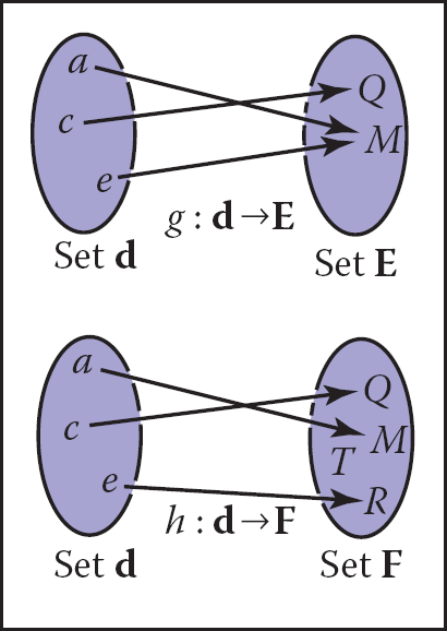
The function g does not have an inverse because two elements of d map to the same element of E. The function h has no inverse because element T of F has no element of d mapped to it.
An example of a bijection is f : ℝ ↦ ℝ, with f(x) = x3. The inverse function is f−1(x)=3√x. This example shows that the standard notation can be somewhat awkward because x is used as a dummy variable in both f and f−1. It is sometimes more intuitive to use different dummy variables, with y = f (x) and x = f−1 (y). This yields the more intuitive y = x3 and x=3√y. An example of a function that does not have an inverse is sqr : ℝ ↦ ℝ, where sqr(x) = x2. This is true for two reasons: first x2 = (−x)2, and second no members of the domain map to the negative portions of the target. Note that we can define an inverse if we restrict the domain and range to ℝ+. Then √x is a valid inverse.
2.1.2 Intervals
Often we would like to specify that a function deals with real numbers that are restricted in value. One such constraint is to specify an interval. An example of an interval is the real numbers between zero and one, not including zero or one. We denote this (0, 1). Because it does not include its endpoints, this is referred to as an open interval. The corresponding closed interval, which does contain its endpoints, is denoted with square brackets: [0, 1]. This notation can be mixed, i.e., [0, 1) includes zero but not one. When writing an interval [a, b], we assume that a ≤ b. The three common ways to represent an interval are shown in Figure 2.3. The Cartesian products of intervals are often used. For example, to indicate that a point x is in the unit cube in 3D, we say x ∈ [0, 1]3.

Intervals are particularly useful in conjunction with set operations: intersection, union, and difference. For example, the intersection of two intervals is the set of points they have in common. The symbol ∩ is used for intersection. For example, [3, 5) ∩ [4, 6] = [4,5). For unions, the symbol ∪ is used to denote points in either interval. For example, [3, 5) ∪ [4, 6] = [3, 6]. Unlike the first two operators, the difference operator produces different results depending on argument order. The minus sign is used for the difference operator, which returns the points in the left interval that are not also in the right. For example, [3, 5) − [4, 6] = [3, 4) and [4, 6] − [3, 5) = [5, 6]. These operations are particularly easy to visualize using interval diagrams (Figure 2.4).
![Figure showing interval operations on [3,5) and [4,6].](http://images-20200215.ebookreading.net/23/1/1/9781482229417/9781482229417__fundamentals-of-computer__9781482229417__image__fig2-4.png)
2.1.3 Logarithms
Although not as prevalent today as they were before calculators, logarithms are often useful in problems where equations with exponential terms arise. By definition, every logarithm has a base a. The “log base a” of x is written loga x and is defined as “the exponent to which a must be raised to get x,” i.e.,
y=log ax ⇔ ay=x.
Note that the logarithm base a and the function that raises a to a power are inverses of each other. This basic definition has several consequences:
alog a(x)=x;log a(ax)=x;log a(xy)=log ax+log ay;log a(x/y)=log ax−log ay;log ax=log ablog bx.
When we apply calculus to logarithms, the special number e = 2.718 ... often turns up. The logarithm with base e is called the natural logarithm. We adopt the common shorthand ln to denote it:
In x≡log ex.
Note that the “≡” symbol can be read “is equivalent by definition.” Like π, the special number e arises in a remarkable number of contexts. Many fields use a particular base in addition to e for manipulations and omit the base in their notation, i.e., log x. For example, astronomers often use base 10 and theoretical computer scientists often use base 2. Because computer graphics borrows technology from many fields we will avoid this shorthand.
The derivatives of logarithms and exponents illuminate why the natural logarithm is “natural”:
ddxlog ax=1xln a;ddxax=axln a.
The constant multipliers above are unity only for a = e.
2.2 Solving Quadratic Equations
A quadratic equation has the form
Ax2+Bx+C=0,
where x is a real unknown, and A, B, and C are known constants. If you think of a 2D xy plot with y = Ax2 + Bx + C, the solution is just whatever x values are “zero crossings” in y. Because y = Ax2 + Bx + C is a parabola, there will be zero, one, or two real solutions depending on whether the parabola misses, grazes, or hits the x-axis (Figure 2.5).

The geometric interpretation of the roots of a quadratic equation is the intersection points of a parabola with the x-axis.
To solve the quadratic equation analytically, we first divide by A:
x2+BAx+CA=0.
Then we “complete the square” to group terms:
(x+B2A)2−B24A2+CA=0.
Moving the constant portion to the right-hand side and taking the square root gives
x+B2A=±√B24A2−CA.
Subtracting B/(2A) from both sides and grouping terms with the denominator 2A gives the familiar form:1
x=−B±√B2−4AC2A. (2.1)
Here the “±” symbol means there are two solutions, one with a plus sign and one with a minus sign. Thus 3 ± 1 equals “two or four.” Note that the term that determines the number of real solutions is
D≡B2−4AC,
which is called the discriminant of the quadratic equation. If D > 0, there are two real solutions (also called roots). If D = 0, there is one real solution (a “double” root). If D < 0, there are no real solutions.
For example, the roots of 2x2 + 6x + 4 = 0 are x = −1 and x = −2, and the equation x2+x+1 has no real solutions. The discriminants of these equations are D = 4 and D = −3, respectively, so we expect the number of solutions given. In programs, it is usually a good idea to evaluate D first and return “no roots” without taking the square root if D is negative.
2.3 Trigonometry
In graphics we use basic trigonometry in many contexts. Usually, it is nothing too fancy, and it often helps to remember the basic definitions.
2.3.1 Angles
Although we take angles somewhat for granted, we should return to their definition so we can extend the idea of the angle onto the sphere. An angle is formed between two half-lines (infinite rays stemming from an origin) or directions, and some convention must be used to decide between the two possibilities for the angle created between them as shown in Figure 2.6. An angle is defined by the length of the arc segment it cuts out on the unit circle. A common convention is that the smaller arc length is used, and the sign of the angle is determined by the order in which the two half-lines are specified. Using that convention, all angles are in the range [−π, π].

Two half-lines cut the unit circle into two arcs. The length of either arc is a valid angle “between” the two half-lines. Either we can use the convention that the smaller length is the angle, or that the two halflines are specified in a certain order and the arc that determines angle ϕ is the one swept out counterclockwise from the first to the second half-line.
Each of these angles is the length of the arc of the unit circle that is “cut” by the two directions. Because the perimeter of the unit circle is 2π, the two possible angles sum to 2π. The unit of these arc lengths is radians. Another common unit is degrees, where the perimeter of the circle is 360 degrees. Thus, an angle that is π radians is 180 degrees, usually denoted 180°. The conversion between degrees and radians is
degrees=180πradians;radians=π180degrees.
2.3.2 Trigonometric Functions
Given a right triangle with sides of length a, o, and h, where h is the length of the longest side (which is always opposite the right angle), or hypotenuse, an important relation is described by the Pythagorean theorem:
a2+o2=h2.
You can see that this is true from Figure 2.7, where the big square has area (a+o)2, the four triangles have the combined area 2ao, and the center square has area h2.

Because the triangles and inner square subdivide the larger square evenly, we have 2ao + h2 = (a + o)2, which is easily manipulated to the form above. We define sine and cosine of ϕ as well as the other ratio-based trigonometric expressions:
sin ϕ≡o/h;csc ϕ≡h/o;cos ϕ≡a/h;sec ϕ≡h/atan ϕ≡o/a;cot ϕ≡a/o.
These definitions allow us to set up polar coordinates, where a point is coded as a distance from the origin and a signed angle relative to the positive x-axis (Figure 2.8). Note the convention that angles are in the range ϕ ∈ (−π, π], and that the positive angles are counterclockwise from the positive x-axis. This convention that counterclockwise maps to positive numbers is arbitrary, but it is used in many contexts in graphics so it is worth committing to memory.

Trigonometric functions are periodic and can take any angle as an argument. For example, sin(A) = sin(A + 2π). This means the functions are not invertible when considered with the domain ℝ. This problem is avoided by restricting the range of standard inverse functions, and this is done in a standard way in almost all modern math libraries (e.g., (Plauger, 1991)). The domains and ranges are:
asin : [−1,1]↦[−π/2, π/2];acos : [−1, 1]↦[0,π];atan : ℝ↦[−π/2, π/2];atan2 : ℝ2↦[−π, π]. (2.2)
The last function, atan2(s, c) is often very useful. It takes an s value proportional to sin A and a c value that scales cos A by the same factor and returns A. The factor is assumed to be positive. One way to think of this is that it returns the angle of a 2D Cartesian point (s, c) in polar coordinates (Figure 2.9).

2.3.3 Useful Identities
This section lists without derivation a variety of useful trigonometric identities.
Shifting identities:
sin (−A)=−sin Acos (−A)=cos Atan (−A)=−tan Asin (π/2−A)=cos Acos (π/2−A)=sin Atan (π/2−A)=cot A
Pythagorean identities:
sin 2A+cos 2A=1sec 2A−tan 2A=1cos 2A−cot 2A=1
Addition and subtraction identities:
sin(A+B)=sin Acos B+sin Bcos Asin(A−B)=sin Acos B−sin Bcos Asin (2A)=2sin Acos Acos (A+B)=cos Acos B−sin Asin Bcos (A−B)=cos Acos B+sin Asin Bcos (2A)=cos 2A−sin 2Atan (A+B)=tan A+tan B1−tan Atan Btan (A−B)=tan A−tan B1+tan Atan Btan (2A)=2tan A1−tan 2A
Half-angle identities:
sin 2(A/2)=(1−cos A)/2cos 2(A/2)=(1+cos A)/2
Product identities:
sin Asin B=−(cos (A+B)−cos (A−B))/2sin Acos B=(sin (A+B)+sin (A−B))/2cos Acos B=(cos (A+B)+cos (A−B))/2
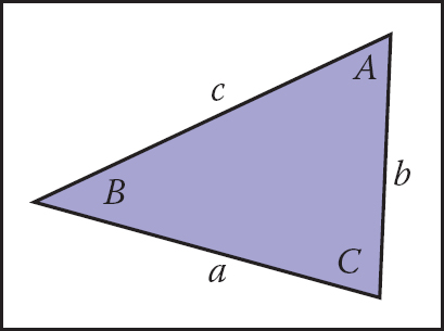
The following identities are for arbitrary triangles with side lengths a, b, and c, each with an angle opposite it given by A, B, C, respectively (Figure 2.10):
The area of a triangle can also be computed in terms of these side lengths:
2.4 Vectors
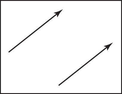
A vector describes a length and a direction. It can be usefully represented by an arrow. Two vectors are equal if they have the same length and direction even if we think of them as being located in different places (Figure 2.11). As much as possible, you should think of a vector as an arrow and not as coordinates or numbers. At some point we will have to represent vectors as numbers in our programs, but even in code they should be manipulated as objects and only the low-level vector operations should know about their numeric representation (DeRose, 1989). Vectors will be represented as bold characters, e.g., a. A vector’s length is denoted ∥a∥. A unit vector is any vector whose length is one. The zero vector is the vector of zero length. The direction of the zero vector is undefined.
Vectors can be used to represent many different things. For example, they can be used to store an offset, also called a displacement. If we know “the treasure is buried two paces east and three paces north of the secret meeting place,” then we know the offset, but we don’t know where to start. Vectors can also be used to store a location, another word for position or point. Locations can be represented as a displacement from another location. Usually there is some understood origin location from which all other locations are stored as offsets. Note that locations are not vectors. As we shall discuss, you can add two vectors. However, it usually does not make sense to add two locations unless it is an intermediate operation when computing weighted averages of a location (Goldman, 1985). Adding two offsets does make sense, so that is one reason why offsets are vectors. But this emphasizes that a location is not an offset; it is an offset from a specific origin location. The offset by itself is not the location.
2.4.1 Vector Operations
Vectors have most of the usual arithmetic operations that we associate with real numbers. Two vectors are equal if and only if they have the same length and direction. Two vectors are added according to the parallelogram rule. This rule states that the sum of two vectors is found by placing the tail of either vector against the head of the other (Figure 2.12). The sum vector is the vector that “completes the triangle” started by the two vectors. The parallelogram is formed by taking the sum in either order. This emphasizes that vector addition is commutative:

Note that the parallelogram rule just formalizes our intuition about displacements. Think of walking along one vector, tail to head, and then walking along the other. The net displacement is just the parallelogram diagonal. You can also create a unary minus for a vector: −a (Figure 2.13) is a vector with the same length as a but opposite direction. This allows us to also define subtraction:

You can visualize vector subtraction with a parallelogram (Figure 2.14). We can write

Vectors can also be multiplied. In fact, there are several kinds of products involving vectors. First, we can scale the vector by multiplying it by a real number k. This just multiplies the vector’s length without changing its direction. For example, 3.5a is a vector in the same direction as a but it is 3.5 times as long as a. We discuss two products involving two vectors, the dot product and the cross product, later in this section, and a product involving three vectors, the determinant, in Chapter 5.
2.4.2 Cartesian Coordinates of a Vector
A 2D vector can be written as a combination of any two nonzero vectors which are not parallel. This property of the two vectors is called linear independence. Two linearly independent vectors form a 2D basis, and the vectors are thus referred to as basis vectors. For example, a vector c may be expressed as a combination of two basis vectors a and b (Figure 2.15):

Note that the weights ac and bc are unique. Bases are especially useful if the two vectors are orthogonal, i.e., they are at right angles to each other. It is even more useful if they are also unit vectors in which case they are orthonormal. If we assume two such “special” vectors x and y are known to us, then we can use them to represent all other vectors in a Cartesian coordinate system, where each vector is represented as two real numbers. For example, a vector a might be represented as
where xa and ya are the real Cartesian coordinates of the 2D vector a (Figure 2.16). Note that this is not really any different conceptually from Equation (2.3), where the basis vectors were not orthonormal. But there are several advantages to a Cartesian coordinate system. For instance, by the Pythagorean theorem, the length of a is

It is also simple to compute dot products, cross products, and coordinates of vectors in Cartesian systems, as we’ll see in the following sections.
By convention we write the coordinates of a either as an ordered pair (xa, ya) or a column matrix:
The form we use will depend on typographic convenience. We will also occasionally write the vector as a row matrix, which we will indicate as aT:
We can also represent 3D, 4D, etc., vectors in Cartesian coordinates. For the 3D case, we use a basis vector z that is orthogonal to both x and y.
2.4.3 Dot Product
The simplest way to multiply two vectors is the dot product. The dot product of a and b is denoted a · b and is often called the scalar product because it returns a scalar. The dot product returns a value related to its arguments’ lengths and the angle ϕ between them (Figure 2.17):

The dot product is related to length and angle and is one of the most important formulas in graphics.
The most common use of the dot product in graphics programs is to compute the cosine of the angle between two vectors.
The dot product can also be used to find the projection of one vector onto another. This is the length a→b of a vector a that is projected at right angles onto a vector b (Figure 2.18):

The dot product obeys the familiar associative and distributive properties we have in real arithmetic:
If 2D vectors a and b are expressed in Cartesian coordinates, we can take advantage of x · x = y · y = 1 and x · y = 0 to derive that their dot product is
Similarly in 3D we can find
2.4.4 Cross Product
The cross product a × b is usually used only for three-dimensional vectors; generalized cross products are discussed in references given in the chapter notes. The cross product returns a 3D vector that is perpendicular to the two arguments of the cross product. The length of the resulting vector is related to sin ϕ:
The magnitude ∥a × b∥ is equal to the area of the parallelogram formed by vectors a and b. In addition, a × b is perpendicular to both a and b (Figure 2.19). Note that there are only two possible directions for such a vector. By definition, the vectors in the direction of the x-, y- and z-axes are given by

The cross product a × b is a 3D vector perpendicular to both 3D vectors a and b, and its length is equal to the area of the parallelogram shown.
and we set as a convention that x × y must be in the plus or minus z direction. The choice is somewhat arbitrary, but it is standard to assume that
All possible permutations of the three Cartesian unit vectors are
Because of the sin ϕ property, we also know that a vector cross itself is the zero-vector, so x × x = 0 and so on. Note that the cross product is not commutative, i.e., x × y ≠ y × x. The careful observer will note that the above discussion does not allow us to draw an unambiguous picture of how the Cartesian axes relate. More specifically, if we put x and y on a sidewalk, with x pointing east and y pointing north, then does z point up to the sky or into the ground? The usual convention is to have z point to the sky. This is known as a right-handed coordinate system. This name comes from the memory scheme of “grabbing” x with your right palm and fingers and rotating it toward y. The vector z should align with your thumb. This is illustrated in Figure 2.20.

The “right-hand rule” for cross products. Imagine placing the base of your right palm where a and b join at their tails, and pushing the arrow of a toward b. Your extended right thumb should point toward a × b.
The cross product has the nice property that
and
However, a consequence of the right-hand rule is
In Cartesian coordinates, we can use an explicit expansion to compute the cross product:
So, in coordinate form,
2.4.5 Orthonormal Bases and Coordinate Frames
Managing coordinate systems is one of the core tasks of almost any graphics program; the key to this is managing orthonormal bases. Any set of two 2D vectors u and v form an orthonormal basis provided that they are orthogonal (at right angles) and are each of unit length. Thus,
In 3D, three vectors u, v, and w form an orthonormal basis if
and
This orthonormal basis is right-handed provided
and otherwise it is left-handed.
Note that the Cartesian canonical orthonormal basis is just one of infinitely many possible orthonormal bases. What makes it special is that it and its implicit origin location are used for low-level representation within a program. Thus, the vectors x, y, and z are never explicitly stored and neither is the canonical origin location o. The global model is typically stored in this canonical coordinate system, and it is thus often called the global coordinate system. However, if we want to use another coordinate system with origin p and orthonormal basis vectors u, v, and w, then we do store those vectors explicitly. Such a system is called a frame of reference or coordinate frame. For example, in a flight simulator, we might want to maintain a coordinate system with the origin at the nose of the plane, and the orthonormal basis aligned with the airplane. Simultaneously, we would have the master canonical coordinate system (Figure 2.21). The coordinate system associated with a particular object, such as the plane, is usually called a local coordinate system.

There is always a master or “canonical” coordinate system with origin o and orthonormal basis x, y, and z. This coordinate system is usually defined to be aligned to the global model and is thus often called the “global” or “world” coordinate system. This origin and basis vectors are never stored explicitly. All other vectors and locations are stored with coordinates that relate them to the global frame. The coordinate system associated with the plane are explicitly stored in terms of global coordinates.
At a low level, the local frame is stored in canonical coordinates. For example, if u has coordinates (xu, yu, zu),
A location implicitly includes an offset from the canonical origin:
where (xp, yp, zp) are the coordinates of p.
Note that if we store a vector a with respect to the u-v-w frame, we store a triple (ua, va, wa) which we can interpret geometrically as
To get the canonical coordinates of a vector a stored in the u-v-w coordinate system, simply recall that u, v, and w are themselves stored in terms of Cartesian coordinates, so the expression uau + vav + waw is already in Cartesian coordinates if evaluated explicitly. To get the u-v-w coordinates of a vector b stored in the canonical coordinate system, we can use dot products:
This works because we know that for some ub, vb, and wb,
and the dot product isolates the ub coordinate:
This works because u, v, and w are orthonormal.
Using matrices to manage changes of coordinate systems is discussed in Sections 6.2.1 and 6.5.
2.4.6 Constructing a Basis from a Single Vector
Often we need an orthonormal basis that is aligned with a given vector. That is, given a vector a, we want an orthonormal u, v, and w such that w points in the same direction as a (Hughes & Möller, 1999), but we don’t particularly care what u and v are. One vector isn’t enough to uniquely determine the answer; we just need a robust procedure that will find any one of the possible bases.
This can be done using cross products as follows. First make w a unit vector in the direction of a:
Then choose any vector t not collinear with w, and use the cross product to build a unit vector u perpendicular to w:
If t is collinear with w the denominator will vanish, and if they are nearly collinear the results will have low precision. A simple procedure to find a vector sufficiently different from w is to start with t equal to w and change the smallest magnitude component of t to 1. For example, if then . Once w and u are in hand, completing the basis is simple:
An example of a situation where this construction is used is surface shading, where a basis aligned to the surface normal is needed but the rotation around the normal is often unimportant.
2.4.7 Constructing a Basis from Two Vectors
The procedure in the previous section can also be used in situations where the rotation of the basis around the given vector is important. A common example is building a basis for a camera: it’s important to have one vector aligned in the direction the camera is looking, but the orientation of the camera around that vector is not arbitrary, and it needs to be specified somehow. Once the orientation is pinned down, the basis is completely determined.
A common way to fully specify a frame is by providing two vectors a (which specifies w) and b (which specifies v). If the two vectors are known to be perpendicular it is a simple matter to construct the third vector by u = b × a.
To be sure that the resulting basis really is orthonormal, even if the input vectors weren’t quite, a procedure much like the single-vector procedure is advisable:
In fact, this procedure works just fine when a and b are not perpendicular. In this case, w will be constructed exactly in the direction of a, and v is chosen to be the closest vector to b among all vectors perpendicular to w.
This procedure won’t work if a and b are collinear. In this case b is of no help in choosing which of the directions perpendicular to a we should use: it is perpendicular to all of them.
In the example of specifying camera positions (Section 4.3), we want to construct a frame that has w parallel to the direction the camera is looking, and v should point out the top of the camera. To orient the camera upright, we build the basis around the view direction, using the straight-up direction as the reference vector to establish the camera’s orientation around the view direction. Setting v as close as possible to straight up exactly matches the intuitive notion of “holding the camera straight.”
2.4.8 Squaring Up a Basis
Occasionally you may find problems caused in your computations by a basis that is supposed to be orthonormal but where error has crept in—due to rounding error in computation, or to the basis having been stored in a file with low precision, for instance.
The procedure of the previous section can be used; simply constructing the basis anew using the existing w and v vectors will produce a new basis that is orthonormal and is close to the old one.
This approach is good for many applications, but it is not the best available. It does produce accurately orthogonal vectors, and for nearly orthogonal starting bases the result will not stray far from the starting point. However, it is asymmetric: it “favors” w over v and v over u (whose starting value is thrown away). It chooses a basis close to the starting basis but has no guarantee of choosing the closest orthonormal basis. When this is not good enough, the SVD (Section 5.4.1) can be used to compute an orthonormal basis that is guaranteed to be closest to the original basis.
2.5 Curves and Surfaces
The geometry of curves, and especially surfaces, plays a central role in graphics, and here we review the basics of curves and surfaces in 2D and 3D space.
2.5.1 2D Implicit Curves
Intuitively, a curve is a set of points that can be drawn on a piece of paper without lifting the pen. A common way to describe a curve is using an implicit equation. An implicit equation in two dimensions has the form
The function f(x, y) returns a real value. Points (x, y) where this value is zero are on the curve, and points where the value is nonzero are not on the curve. For example, let’s say that f(x, y) is
where (xc, yc) is a 2D point and r is a nonzero real number. If we take f(x, y) = 0, the points where this equality holds are on the circle with center (xc, yc) and radius r. The reason that this is called an “implicit” equation is that the points (x, y) on the curve cannot be immediately calculated from the equation and instead must be determined by solving the equation. Thus, the points on the curve are not generated by the equation explicitly, but they are buried somewhere implicitly in the equation.
It is interesting to note that f does have values for all (x, y). We can think of f as a terrain, with sea level at f = 0 (Figure 2.22). The shore is the implicit curve. The value of f is the altitude. Another thing to note is that the curve partitions space into regions where f > 0, f < 0, and f = 0. So you evaluate f to decide whether a point is “inside” a curve. Note that f(x, y) = c is a curve for any constant c, and c = 0 is just used as a convention. For example, if f(x, y) = x2 + y2 −1, varying c just gives a variety of circles centered at the origin (Figure 2.23).

An implicit function f(x,y) = 0 can be thought of as a height field where f is the height (top). A path where the height is zero is the implicit curve (bottom).

An implicit function f(x,y) = 0 can be thought of as a height field where f is the height (top). A path where the height is zero is the implicit curve (bottom).
We can compress our notation using vectors. If we have c = (xc, yc) and p = (x, y), then our circle with center c and radius r is defined by those position vectors that satisfy
This equation, if expanded algebraically, will yield Equation (2.9), but it is easier to see that this is an equation for a circle by “reading” the equation geometrically. It reads, “points p on the circle have the following property: the vector from c to p when dotted with itself has value r2.” Because a vector dotted with itself is just its own length squared, we could also read the equation as, “points p on the circle have the following property: the vector from c to p has squared length r2.”
Even better, is to observe that the squared length is just the squared distance from c to p, which suggests the equivalent form
and, of course, this suggests
The above could be read “the points p on the circle are those a distance r from the center point c,” which is as good a definition of circle as any. This illustrates that the vector form of an equation often suggests more geometry and intuition than the equivalent full-blown Cartesian form with x and y. For this reason, it is usually advisable to use vector forms when possible. In addition, you can support a vector class in your code; the code is cleaner when vector forms are used. The vector-oriented equations are also less error prone in implementation: once you implement and debug vector types in your code, the cut-and-paste errors involving x, y, and z will go away. It takes a little while to get used to vectors in these equations, but once you get the hang of it, the payoff is large.
2.5.2 The 2D Gradient
If we think of the function f (x, y) as a height field with height = f (x, y), the gradient vector points in the direction of maximum upslope, i.e., straight uphill. The gradient vector ∇ f (x, y) is given by
The gradient vector evaluated at a point on the implicit curve f (x, y) = 0 is perpendicular to the tangent vector of the curve at that point. This perpendicular vector is usually called the normal vector to the curve. In addition, since the gradient points uphill, it indicates the direction of the f (x, y) > 0 region.
In the context of height fields, the geometric meaning of partial derivatives and gradients is more visible than usual. Suppose that near the point (a, b), f (x, y) is a plane (Figure 2.24). There is a specific uphill and downhill direction. At right angles to this direction is a direction that is level with respect to the plane. Any intersection between the plane and the f (x, y) = 0 plane will be in the direction that is level. Thus the uphill/downhill directions will be perpendicular to the line of intersection f (x, y) = 0. To see why the partial derivative has something to do with this, we need to visualize its geometric meaning. Recall that the conventional derivative of a 1D function y = g(x) is

A surface height = f (x,y) is locally planar near (x,y) = (a,b). The gradient is a projection of the uphill direction onto the height = 0 plane.
This measures the slope of the tangent line to g (Figure 2.25).
The partial derivative is a generalization of the 1D derivative. For a 2D function f(x, y), we can’t take the same limit for x as in Equation (2.10), because f can change in many ways for a given change in x. However, if we hold y constant, we can define an analog of the derivative, called the partial derivative (Figure 2.26):

The partial derivative of a function f with respect to x must hold y constant to have a unique value, as shown by the dark point. The hollow points show other values of f that do not hold y constant.
Why is it that the partial derivatives with respect to x and y are the components of the gradient vector? Again, there is more obvious insight in the geometry than in the algebra. In Figure 2.27, we see the vector a travels along a path where f does not change. Note that this is again at a small enough scale that the surface height (x, y) = f(x, y) can be considered locally planar. From the figure, we see that the vector a = (Δx, Δy).

The vector a points in a direction where f has no change and is thus perpendicular to the gradient vector ∇f.
Because the uphill direction is perpendicular to a, we know the dot product is equal to zero:
We also know that the change in f in the direction (xa, ya) equals zero:
Given any vectors (x, y) and (x′, y′) that are perpendicular, we know that the angle between them is 90 degrees, and thus their dot product equals zero (recall that the dot product is proportional to the cosine of the angle between the two vectors). Thus, we have xx′ + yy′ = 0. Given (x,y), it is easy to construct valid vectors whose dot product with (x, y) equals zero, the two most obvious being (y, −x) and (−y,x); you can verify that these vectors give the desired zero dot product with (x, y). A generalization of this observation is that (x, y) is perpendicular to k(y, −x) where k is any nonzero constant. This implies that
Combining Equations (2.11) and (2.12) gives
where k′ is any nonzero constant. By definition, “uphill” implies a positive change in f, so we would like k′ > 0, and k′ = 1 is a perfectly good convention.
As an example of the gradient, consider the implicit circle x2 + y2 − 1 = 0 with gradient vector (2x, 2y), indicating that the outside of the circle is the positive region for the function f (x, y) = x2 + y2 − 1. Note that the length of the gradient vector can be different depending on the multiplier in the implicit equation. For example, the unit circle can be described by Ax2 + Ay2 − A = 0 for any nonzero a. The gradient for this curve is (2Ax, 2Ay). This will be normal (perpendicular) to the circle, but will have a length determined by a. For A > 0, the normal will point outward from the circle, and for A < 0, it will point inward. This switch from outward to inward is as it should be, since the positive region switches inside the circle. In terms of the height-field view, h = Ax2 + Ay2 − A, and the circle is at zero altitude. For A > 0, the circle encloses a depression, and for A < 0, the circle encloses a bump. As A becomes more negative, the bump increases in height, but the h = 0 circle doesn’t change. The direction of maximum uphill doesn’t change, but the slope increases. The length of the gradient reflects this change in degree of the slope. So intuitively, you can think of the gradient’s direction as pointing uphill and its magnitude as measuring how uphill the slope is.
Implicit 2D Lines
The familiar “slope-intercept” form of the line is
This can be converted easily to implicit form (Figure 2.28):

Here m is the “slope” (ratio of rise to run) and b is the y value where the line crosses the y-axis, usually called the y-intercept. The line also partitions the 2D plane, but here “inside” and “outside” might be more intuitively called “over” and “under.”
Because we can multiply an implicit equation by any constant without changing the points where it is zero, kf(x, y) = 0 is the same curve for any nonzero k. This allows several implicit forms for the same line, for example,
One reason the slope-intercept form is sometimes awkward is that it can’t represent some lines such as x = 0 because m would have to be infinite. For this reason, a more general form is often useful:
for real numbers A, B, C.
Suppose we know two points on the line, (x0, y0) and (x1, y1). What A, B, and C describe the line through these two points? Because these points lie on the line, they must both satisfy Equation (2.15):
Unfortunately we have two equations and three unknowns: A, B, and C. This problem arises because of the arbitrary multiplier we can have with an implicit equation. We could set C = 1 for convenience:
but we have a similar problem to the infinite slope case in slope-intercept form: lines through the origin would need to have A(0) + B(0) + 1 = 0, which is a contradiction. For example, the equation for a 45-degree line through the origin can be written x − y = 0, or equally well y − x = 0, or even 17y − 17x = 0, but it cannot be written in the form Ax + By + 1 = 0.
Whenever we have such pesky algebraic problems, we try to solve the problems using geometric intuition as a guide. One tool we have, as discussed in Section 2.5.2, is the gradient. For the line Ax + By + C = 0, the gradient vector is (A, B). This vector is perpendicular to the line (Figure 2.29), and points to the side of the line where Ax + By + C is positive. Given two points on the line (x0, y0) and (x1, y1), we know that the vector between them points in the same direction as the line. This vector is just (x1 − x0, y1 − y0), and because it is parallel to the line, it must also be perpendicular to the gradient vector (A, B). Recall that there are an infinite number of (A, B, C) that describe the line because of the arbitrary scaling property of implicits. We want any one of the valid (A, B, C).

We can start with any (A, B) perpendicular to (x1 − x0, y1 − y0). Such a vector is just (A, B) = (y0 − y1, x1 − x0) by the same reasoning as in Section 2.5.2. This means that the equation of the line through (x0, y0) and (x1, y1) is
Now we just need to find C. Because (x0, y0) and (x1, y1) are on the line, they must satisfy Equation (2.16). We can plug either value in and solve for C. Doing this for (x0, y0) yields C = x0y1 − x1y0, and thus the full equation for the line is
Again, this is one of infinitely many valid implicit equations for the line through two points, but this form has no division operation and thus no numerically degenerate cases for points with finite Cartesian coordinates. A nice thing about Equation (2.17) is that we can always convert to the slope-intercept form (when it exists) by moving the non-y terms to the right-hand side of the equation and dividing by the multiplier of the y term:
An interesting property of the implicit line equation is that it can be used to find the signed distance from a point to the line. The value of Ax + By + C is proportional to the distance from the line (Figure 2.30). As shown in Figure 2.31, the distance from a point to the line is the length of the vector k(A, B), which is

The value of the implicit function f (x,y) = Ax + By + C is a constant times the signed distance from Ax + By + C = 0.

The vector k(A,B) connects a point (x,y) on the line closest to a point not on the line. The distance is proportional to k.
For the point (x, y) + k(A, B), the value of f (x, y) = Ax + By + C is
The simplification in that equation is a result of the fact that we know (x, y) is on the line, so Ax + By + C = 0. From Equations (2.18) and (2.19), we can see that the signed distance from line Ax + By + C = 0 to a point (a, b) is
Here “signed distance” means that its magnitude (absolute value) is the geometric distance, but on one side of the line, distances are positive and on the other they are negative. You can choose between the equally valid representations f (x, y) = 0 and − f (x, y) = 0 if your problem has some reason to prefer a particular side being positive. Note that if (A, B) is a unit vector, then f (a, b) is the signed distance. We can multiply Equation (2.17) by a constant that ensures that (A, B) is a unit vector:
Note that evaluating f (x, y) in Equation (2.20) directly gives the signed distance, but it does require a square root to set up the equation. Implicit lines will turn out to be very useful for triangle rasterization (Section 8.1.2). Other forms for 2D lines are discussed in Chapter 14.
Implicit Quadric Curves
In the previous section we saw that a linear function f (x, y) gives rise to an implicit line f (x, y) = 0. If f is instead a quadratic function of x and y, with the general form
the resulting implicit curve is called a quadric. Two-dimensional quadric curves include ellipses and hyperbolas, as well as the special cases of parabolas, circles, and lines.
Examples of quadric curves include the circle with center (xc, yc) and radius r,
and axis-aligned ellipses of the form
where (xc, yc) is the center of the ellipse, and a and b are the minor and major semi-axes (Figure 2.32).

2.5.3 3D Implicit Surfaces
Just as implicit equations can be used to define curves in 2D, they can be used to define surfaces in 3D. As in 2D, implicit equations implicitly define a set of points that are on the surface:
Any point (x, y, z) that is on the surface results in zero when given as an argument to f. Any point not on the surface results in some number other than zero. You can check whether a point is on the surface by evaluating f, or you can check which side of the surface the point lies on by looking at the sign of f, but you cannot always explicitly construct points on the surface. Using vector notation, we will write such functions of p = (x, y, z) as
2.5.4 Surface Normal to an Implicit Surface
A surface normal (which is needed for lighting computations, among other things) is a vector perpendicular to the surface. Each point on the surface may have a different normal vector. In the same way that the gradient provides a normal to an implicit curve in 2D, the surface normal at a point p on an implicit surface is given by the gradient of the implicit function
The reasoning is the same as for the 2D case: the gradient points in the direction of fastest increase in f, which is perpendicular to all directions tangent to the surface, in which f remains constant. The gradient vector points toward the side of the surface where f(p) > 0, which we may think of as “into” the surface or “out from” the surface in a given context. If the particular form of f creates inward-facing gradients, and outward-facing gradients are desired, the surface − f(p) = 0 is the same as surface f(p) = 0 but has directionally reversed gradients, i.e., −∇f(p)=∇(−f(p)).
2.5.5 Implicit Planes
As an example, consider the infinite plane through point a with surface normal n. The implicit equation to describe this plane is given by
Note that a and n are known quantities. The point p is any unknown point that satisfies the equation. In geometric terms this equation says “the vector from a to p is perpendicular to the plane normal.” If p were not in the plane, then (p − a) would not make a right angle with n (Figure 2.33).
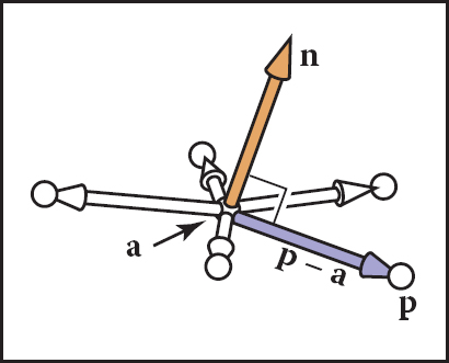
Any of the points p shown are in the plane with normal vector n that includes point a if Equation (2.2) is satisfied.
Sometimes we want the implicit equation for a plane through points a, b, and c. The normal to this plane can be found by taking the cross product of any two vectors in the plane. One such cross product is
This allows us to write the implicit plane equation:
A geometric way to read this equation is that the volume of the parallelepiped defined by p − a, b − a, and c − a is zero, i.e., they are coplanar. This can only be true if p is in the same plane as a, b, and c. The full-blown Cartesian representation for this is given by the determinant (this is discussed in more detail in Section 5.3):
The determinant can be expanded (see Section 5.3 for the mechanics of expanding determinants) to the bloated form with many terms.
Equations (2.22) and (2.23) are equivalent, and comparing them is instructive. Equation (2.22) is easy to interpret geometrically and will yield efficient code. In addition, it is relatively easy to avoid a typographic error that compiles into incorrect code if it takes advantage of debugged cross and dot product code. Equation (2.23) is also easy to interpret geometrically and will be efficient provided an efficient 3 × 3 determinant function is implemented. It is also easy to implement without a typo if a function determinant (a, b, c) is available. It will be especially easy for others to read your code if you rename the determinant function volume. So both Equations (2.22) and (2.23) map well into code. The full expansion of either equation into x-, y-, and z-components is likely to generate typos. Such typos are likely to compile and, thus, to be especially pesky. This is an excellent example of clean math generating clean code and bloated math generating bloated code.
3D Quadric Surfaces
Just as quadratic polynomials in two variables define quadric curves in 2D, quadratic polynomials in x, y, and z define quadric surfaces in 3D. For instance, a sphere can be written as
and an axis-aligned ellipsoid may be written as
3D Curves from Implicit Surfaces
One might hope that an implicit 3D curve could be created with the form f(p) = 0. However, all such curves are just degenerate surfaces and are rarely useful in practice. A 3D curve can be constructed from the intersection of two simultaneous implicit equations:
For example, a 3D line can be formed from the intersection of two implicit planes. Typically, it is more convenient to use parametric curves instead; they are discussed in the following sections.
2.5.6 2D Parametric Curves
A parametric curve is controlled by a single parameter that can be considered a sort of index that moves continuously along the curve. Such curves have the form
Here (x, y) is a point on the curve, and t is the parameter that influences the curve. For a given t, there will be some point determined by the functions g and h. For continuous g and h, a small change in t will yield a small change in x and y. Thus, as t continuously changes, points are swept out in a continuous curve. This is a nice feature because we can use the parameter t to explicitly construct points on the curve. Often we can write a parametric curve in vector form,
where f is a vector-valued function, f : ℝ ↦ ℝ2. Such vector functions can generate very clean code, so they should be used when possible.
We can think of the curve with a position as a function of time. The curve can go anywhere and could loop and cross itself. We can also think of the curve as having a velocity at any point. For example, the point p(t) is traveling slowly near t = − 2 and quickly between t = 2 and t = 3. This type of “moving point” vocabulary is often used when discussing parametric curves even when the curve is not describing a moving point.
2D Parametric Lines
A parametric line in 2D that passes through points p0 = (x0,y0) and p1 = (x1,y1) can be written as
Because the formulas for x and y have such similar structure, we can use the vector form for p = (x, y) (Figure 2.34):
![Figure showing a 2D parametric line through p0 and p1. The line segment defined by t ∈ [0,1] is shown in bold.](http://images-20200215.ebookreading.net/23/1/1/9781482229417/9781482229417__fundamentals-of-computer__9781482229417__image__fig2-34.png)
A 2D parametric line through p0 and p1. The line segment defined by t ∈ [0,1] is shown in bold.
You can read this in geometric form as: “start at point p0 and go some distance toward p1 determined by the parameter t.” A nice feature of this form is that p(0) = p0 and p(1) = p1. Since the point changes linearly with t, the value of t between p0 and p1 measures the fractional distance between the points. Points with t < 0 are to the “far” side of p0, and points with t > 1 are to the “far” side of p1.
Parametric lines can also be described as just a point o and a vector d:
When the vector d has unit length, the line is arc-length parameterized. This means t is an exact measure of distance along the line. Any parametric curve can be arc-length parameterized, which is obviously a very convenient form, but not all can be converted analytically.
2D Parametric Circles
A circle with center (xc, yc) and radius r has a parametric form:
To ensure that there is a unique parameter ϕ for every point on the curve, we can restrict its domain: ϕ ∈ [0, 2π) or ϕ ∈ (−π, π] or any other half-open interval of length 2π.
An axis-aligned ellipse can be constructed by scaling the x and y parametric equations separately:
2.5.7 3D Parametric Curves
A 3D parametric curve operates much like a 2D parametric curve:
For example, a spiral around the z-axis is written as:
As with 2D curves, the functions f, g, and h are defined on a domain D ⊂ ℝ if we want to control where the curve starts and ends. In vector form we can write
In this chapter we only discuss 3D parametric lines in detail. General 3D parametric curves are discussed more extensively in Chapter 15.
3D Parametric Lines
A 3D parametric line can be written as a straightforward extension of the 2D parametric line, e.g.,
This is cumbersome and does not translate well to code variables, so we will write it in vector form:
where, for this example, o and d are given by
Note that this is very similar to the 2D case. The way to visualize this is to imagine that the line passes through o and is parallel to d. Given any value of t, you get some point p(t) on the line. For example, at t = 2, p(t) = (2,1, 3) + 2(7, 2, −5) = (16, 5, −7). This general concept is the same as for two dimensions (Figure 2.30).
As in 2D, a line segment can be described by a 3D parametric line and an interval t ∈ [ta, tb]. The line segment between two points a and b is given by p(t) = a + t(b − a) with t ∈ [0,1]. Here p(0) = a, p(1) = b, and p(0.5) = (a + b)/2, the midpoint between a and b.
A ray, or half-line, is a 3D parametric line with a half-open interval, usually [0, ∞). From now on we will refer to all lines, line segments, and rays as “rays.” This is sloppy, but corresponds to common usage and makes the discussion simpler.
2.5.8 3D Parametric Surfaces
The parametric approach can be used to define surfaces in 3D space in much the same way we define curves, except that there are two parameters to address the two-dimensional area of the surface. These surfaces have the form
or, in vector form,
Example.
For example, a point on the surface of the Earth can be described by the two parameters longitude and latitude. If we define the origin to be at the center of the Earth, and let r be the radius of the Earth, then a spherical coordinate system centered at the origin (Figure 2.35), lets us derive the parametric equations

Ideally, we’d like to write this in vector form, but it isn’t feasible for this particular parametric form.
We would also like to be able to find the (θ, ϕ) for a given (x, y, z). If we assume that ϕ ∈ (−π, π] this is easy to do using the atan2 function from Equation (2.2):
With implicit surfaces, the derivative of the function f gave us the surface normal. With parametric surfaces, the derivatives of p also give information about the surface geometry.
Consider the function q(t) = p(t,v0). This function defines a parametric curve obtained by varying u while holding v fixed at the value v0. This curve, called an isoparametric curve (or sometimes “isoparm” for short) lies in the surface. The derivative of q gives a vector tangent to the curve, and since the curve lies in the surface the vector q′ also lies in the surface. Since it was obtained by varying one argument of p, the vector q′ is the partial derivative of p with respect to u, which we’ll denote pu. A similar argument shows that the partial derivative pv gives the tangent to the isoparametric curves for constant u, which is a second tangent vector to the surface.
The derivative of p, then, gives two tangent vectors at any point on the surface. The normal to the surface may be found by taking the cross product of these vectors: since both are tangent to the surface, their cross product, which is perpendicular to both tangents, is normal to the surface. The right-hand rule for cross products provides a way to decide which side is the front, or outside, of the surface; we will use the convention that the vector
points toward the outside of the surface.
2.5.9 Summary of Curves and Surfaces
Implicit curves in 2D or surfaces in 3D are defined by scalar-valued functions of two or three variables, f : ℝ2 → ℝ or f : ℝ3 → ℝ, and the surface consists of all points where the function is zero:
Parametric curves in 2D or 3D are defined by vector-valued functions of one variable, p : D ⊂ ℝ → ℝ2 or p: D⊂ ℝ → ℝ3, and the curve is swept out as t varies over all of D:
Parametric surfaces in 3D are defined by vector-valued functions of two variables, p : D ⊂ ℝ2 → ℝ3, and the surface consists of the images of all points (u, v) in the domain:
For implicit curves and surfaces, the normal vector is given by the derivative of f (the gradient), and the tangent vector (for a curve) or vectors (for a surface) can be derived from the normal by constructing a basis.
For parametric curves and surfaces, the derivative of p gives the tangent vector (for a curve) or vectors (for a surface), and the normal vector can be derived from the tangents by constructing a basis.
2.6 Linear Interpolation
Perhaps the most common mathematical operation in graphics is linear interpolation. We have already seen an example of linear interpolation of position to form line segments in 2D and 3D, where two points a and b are associated with a parameter t to form the line p = (1 − t)a + tb. This is interpolation because p goes through a and b exactly at t = 0 and t = 1. It is linear interpolation because the weighting terms t and 1 — t are linear polynomials of t.
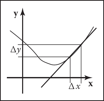
Another common linear interpolation is among a set of positions on the x-axis: x0, x1, ..., xn, and for each xi we have an associated height, yi. We want to create a continuous function y = f (x) that interpolates these positions, so that f goes through every data point, i.e., f(xi) = yi. For linear interpolation, the points (xi, yi) are connected by straight line segments. It is natural to use parametric line equations for these segments. The parameter t is just the fractional distance between xi and xi+1:
Because the weighting functions are linear polynomials of x, this is linear interpolation.
The two examples above have the common form of linear interpolation. We create a variable t that varies from 0 to 1 as we move from data item A to data item B. Intermediate values are just the function (1 − t)A + tB. Notice that Equation (2.26) has this form with
2.7 Triangles
Triangles in both 2D and 3D are the fundamental modeling primitive in many graphics programs. Often information such as color is tagged onto triangle vertices, and this information is interpolated across the triangle. The coordinate system that makes such interpolation straightforward is called barycentric coordinates; we will develop these from scratch. We will also discuss 2D triangles, which must be understood before we can draw their pictures on 2D screens.
2.7.1 2D Triangles
If we have a 2D triangle defined by 2D points a, b, and c, we can first find its area:
The derivation of this formula can be found in Section 5.3. This area will have a positive sign if the points a, b, and c are in counterclockwise order and a negative sign, otherwise.
Often in graphics, we wish to assign a property, such as color, at each triangle vertex and smoothly interpolate the value of that property across the triangle. There are a variety of ways to do this, but the simplest is to use barycentric coordinates. One way to think of barycentric coordinates is as a nonorthogonal coordinate system as was discussed briefly in Section 2.4.2. Such a coordinate system is shown in Figure 2.36, where the coordinate origin is a and the vectors from a to b and c are the basis vectors. With that origin and those basis vectors, any point p can be written as

A 2D triangle with vertices a, b, c can be used to set up a nonorthogonal coordinate system with origin a and basis vectors (b − a) and (c − a). A point is then represented by an ordered pair (β, γ). For example, the point p = (2.0, 0.5), i.e., p = a + 2.0 (b − a) + 0.5 (c − a).
Note that we can reorder the terms in Equation (2.28) to get
Often people define a new variable α to improve the symmetry of the equations:
which yields the equation
with the constraint that
Barycentric coordinates seem like an abstract and unintuitive construct at first, but they turn out to be powerful and convenient. You may find it useful to think of how street addresses would work in a city where there are two sets of parallel streets, but where those sets are not at right angles. The natural system would essentially be barycentric coordinates, and you would quickly get used to them. Barycentric coordinates are defined for all points on the plane. A particularly nice feature of barycentric coordinates is that a point p is inside the triangle formed by a, b, and c if and only if
If one of the coordinates is zero and the other two are between zero and one, then you are on an edge. If two of the coordinates are zero, then the other is one, and you are at a vertex. Another nice property of barycentric coordinates is that Equation (2.29) in effect mixes the coordinates of the three vertices in a smooth way. The same mixing coefficients (α, β, γ) can be used to mix other properties, such as color, as we will see in the next chapter.
Given a point p, how do we compute its barycentric coordinates? One way is to write Equation (2.28) as a linear system with unknowns β and γ, solve, and set α = 1 − β − γ. That linear system is
Although it is straightforward to solve Equation (2.31) algebraically, it is often fruitful to compute a direct geometric solution.
One geometric property of barycentric coordinates is that they are the signed scaled distance from the lines through the triangle sides, as is shown for β in Figure 2.37. Recall from Section 2.5.2 that evaluating the equation f(x, y) for the line f (x, y)=0 returns the scaled signed distance from (x, y) to the line. Also recall that if f (x, y) = 0 is the equation for a particular line, so is kf(x, y) = 0 for any nonzero k. Changing k scales the distance and controls which side of the line has positive signed distance, and which negative. We would like to choose k such that, for example, kf (x, y) = β. Since k is only one unknown, we can force this with one constraint, namely that at point b we know β = 1. So if the line fac(x, y) = 0 goes through both a and c, then we can compute β for a point (x,y) as follows:

The barycentric coordinate β is the signed scaled distance from the line through a and c.
and we can compute γ and α in a similar fashion. For efficiency, it is usually wise to compute only two of the barycentric coordinates directly and to compute the third using Equation (2.30).
To find this “ideal” form for the line through p0 and p1, we can first use the technique of Section 2.5.2 to find some valid implicit lines through the vertices. Equation (2.17) gives us
Note that fab(xc, yc) probably does not equal one, so it is probably not the ideal form we seek. By dividing through by fab(xc, yc) we get
The presence of the division might worry us because it introduces the possibility of divide-by-zero, but this cannot occur for triangles with areas that are not near zero. There are analogous formulas for α and β, but typically only one is needed:
Another way to compute barycentric coordinates is to compute the areas Aa, Ab, and Ac, of subtriangles as shown in Figure 2.38. Barycentric coordinates obey the rule
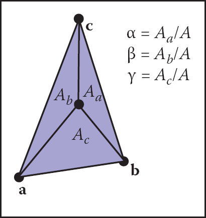
The barycentric coordinates are proportional to the areas of the three subtriangles shown.
where A is the area of the triangle. Note that A = Aa + Ab + Ac, so it can be computed with two additions rather than a full area formula. This rule still holds for points outside the triangle if the areas are allowed to be signed. The reason for this is shown in Figure 2.39. Note that these are signed areas and will be computed correctly as long as the same signed area computation is used for both A and the subtriangles Aa, Ab, and Ac.

The area of the two triangles shown is base times height and are thus the same, as is any triangle with a vertex on the β = 0.5 line. The height and thus the area is proportional to β.
2.7.2 3D Triangles
One wonderful thing about barycentric coordinates is that they extend almost transparently to 3D. If we assume the points a, b, and c are 3D, then we can still use the representation
Now, as we vary β and γ, we sweep out a plane.
The normal vector to a triangle can be found by taking the cross product of any two vectors in the plane of the triangle (Figure 2.40). It is easiest to use two of the three edges as these vectors, for example,

The normal vector of the triangle is perpendicular to all vectors in the plane of the triangle, and thus perpendicular to the edges of the triangle.
Note that this normal vector is not necessarily of unit length, and it obeys the right-hand rule of cross products.
The area of the triangle can be found by taking the length of the cross product:
Note that this is not a signed area, so it cannot be used directly to evaluate barycentric coordinates. However, we can observe that a triangle with a “clockwise” vertex order will have a normal vector that points in the opposite direction to the normal of a triangle in the same plane with a “counterclockwise” vertex order. Recall that
where ϕ is the angle between the vectors. If a and b are parallel, then cos ϕ = ±1, and this gives a test of whether the vectors point in the same or opposite directions. This, along with Equations (2.33), (2.34), and (2.35), suggest the formulas
where n is Equation (2.34) evaluated with vertices a, b, and c; na is Equation (2.34) evaluated with vertices b, c, and p, and so on, i.e.,
Frequently Asked Questions
Why isn’t there vector division?
It turns out that there is no “nice” analogy of division for vectors. However, it is possible to motivate the quaternions by examining this question in detail (see Hoffmann’s book referenced in the chapter notes).
Is there something as clean as barycentric coordinates for polygons with more than three sides?
Unfortunately there is not. Even convex quadrilaterals are much more complicated. This is one reason triangles are such a common geometric primitive in graphics.
Is there an implicit form for 3D lines?
No. However, the intersection of two 3D planes defines a 3D line, so a 3D line can be described by two simultaneous implicit 3D equations.
Notes
The history of vector analysis is particularly interesting. It was largely invented by Grassman in the mid-1800s but was ignored and reinvented later (Crowe, 1994). Grassman now has a following in the graphics field of researchers who are developing Geometric Algebra based on some of his ideas (Doran & Lasenby, 2003). Readers interested in why the particular scalar and vector products are in some sense the right ones, and why we do not have a commonly used vector division, will find enlightenment in the concise About Vectors (Hoffmann, 1975). Another important geometric tool is the quaternion invented by Hamilton in the mid-1800s. Quaternions are useful in many situations, but especially where orientations are concerned (Hanson, 2005).
Exercises
- The cardinality of a set is the number of elements it contains. Under IEEE floating point representation (Section 1.5), what is the cardinality of the floats?
- Is it possible to implement a function that maps 32-bit integers to 64-bit integers that has a well-defined inverse? Do all functions from 32-bit integers to 64-bit integers have well-defined inverses?
- Specify the unit cube (x-, y-, and z-coordinates all between 0 and 1 inclusive) in terms of the Cartesian product of three intervals.
- If you have access to the natural log function ln(x), specify how you could use it to implement a log(b, x) function where b is the base of the log. What should the function do for negative b values? Assume an IEEE floating point implementation.
- Solve the quadratic equation 2x2 + 6x + 4 = 0.
- Implement a function that takes in coefficients A, B, and C for the quadratic equation Ax2 + Bx + C = 0 and computes the two solutions. Have the function return the number of valid (not NaN) solutions and fill in the return arguments so the smaller of the two solutions is first.
- Show that the two forms of the quadratic formula on page 17 are equivalent (assuming exact arithmetic) and explain how to choose one for each root in order to avoid subtracting nearly equal floating point numbers, which leads to loss of precision.
- Show by counterexample that it is not always true that for 3D vectors a, b, and c, a × (b × c) = (a × b) × c.
- Given the nonparallel 3D vectors a and b, compute a right-handed orthonormal basis such that u is parallel to a and v is in the the plane defined by a and b.
- What is the gradient of f(x, y, z) = x2 + y – 3z3?
- What is a parametric form for the axis-aligned 2D ellipse?
- What is the implicit equation of the plane through 3D points (1, 0, 0), (0, 1, 0), and (0, 0, 1)? What is the parametric equation? What is the normal vector to this plane?
- Given four 2D points a0, a1, b0, and b1, design a robust procedure to determine whether the line segments a0a1 and b0b1 intersect.
- Design a robust procedure to compute the barycentric coordinates of a 2D point with respect to three 2D non-collinear points.
1 A robust implementation will use the equivalent expression to compute one of the roots, depending on the sign of B (Exercise 7).