
CHAPTER FOUR
Games in Extensive Form: Sequential Decision Making
History is an account, mostly false, of events, mostly unimportant, which are brought about by rulers, mostly knaves, and soldiers, mostly fools.
—Ambrose Bierce
Not the power to remember, but its very opposite, the power to forget, is a necessary condition for our existence.
—Saint Basil
A game in which each player has a single move and the players choose and play their strategies simultaneously are easy to model and write down in matrix form. Many, if not most games involve many moves by each player, with choices made sequentially, with or without knowledge of the moves an opponent has made. We have already met examples of these games in 2 × 2 Nim and Russian Roulette. The sequential moves lead to complicated strategies which, when played against each other, lead to the matrix of the game. That is called putting the game in strategic, or normal form.
4.1 Introduction to Game Trees—Gambit
In this chapter, we consider games in which player decisions are made simultaneously (as in a matrix game) or sequentially (one after the other), or both. These are interchangeably called sequential games, extensive form games, or dynamic games. When moves are made sequentially various questions regarding the information available to the next mover must be answered. Every game in which the players choose simultaneously can be modeled as a sequential game with no information. Consequently, every matrix game can be viewed as a sequential game. Conversely, every sequential game can be reduced to a matrix game if strategies are defined correctly.
Every sequential game is represented by a game tree. The tree has a starting node and branches to decision nodes, which is when a decision needs to be made by a player. When the end of the decision-making process is complete, the payoffs to each player are computed. Thus, decisions need not be made simultaneously or without knowledge of the other players decisions. In addition, extensive form games can also be used to describe games with simultaneous moves.
Game trees can also be used to incorporate information passed between the players. In a complete (or perfect) information game, players know all there is to know–the moves and payoffs of all players. In other words, each player sees the board and all the moves the opponent has made. In a game with imperfect information, one or both players must make a decision at certain times not knowing the previous move of the other player or the outcome of some random event (like a coin toss). In other words, each player at each decision node will have an information set associated with that node.
If there is more than one node in an information set, then it is a game of incomplete information.
If there is only one node in each information set, it is a game of perfect information.
This chapter presents examples to illustrate the basic concepts, without going into the technical definitions. We rely to a great extent on the software GAMBIT1 to model and solve the games as they get more complicated.
We start with a simple example that illustrates the difference between sequential and simultaneous moves.
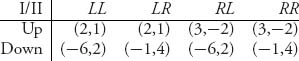
Example 4.1 Two players select a direction. Player I may choose either Up or Down, while player II may choose either Left or Right. Now we look at the two cases when the players choose sequentially, and simultaneously.
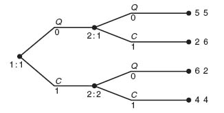
Sequential Moves. Player I goes first, choosing either Up or Down, then player II, knowing player I’s choice, chooses either Left or Right. At the end of each branch, the payoffs are computed.
As in Chapter 1, a strategy is a plan for each player to carry out at whichever node one finds oneself. A strategy for player I, who goes first in this game, is simply Up or Down. The strategies for player II are more complicated because she has to account for player I’s choices.
| LL | If I chooses U, then Left; If I chooses Down, then Left |
| LR | If I chooses U, then Left; If I chooses Down, then Right |
| RL | If I chooses U, then Right; If I chooses Down, then Left |
| RR | If I chooses U, then Right; If I chooses Down, then Right |
Gambit automatically numbers the decision nodes for each player. In the diagram Figure 4.1, 2: 1 means that this is node 1 and information set 1 for player II; 2: 2 signifies information set 2 for player II. When each player has a new information set at each node where they have to make a decision, it is a perfect information set game.
Once the tree is constructed and the payoffs calculated this game can be summarized in the matrix, or strategic form of the game,
Now we can analyze the bimatrix game as before. When we use Gambit to analyze the game, it produces Nash equilibria and the corresponding payoffs to each player. On the diagram Figure 4.1 the numbers below the branches represent the probability the player should play that branch. In this case, player I should play Up all the time; player II should play LR all the time. You can see from the matrix that it is a pure Nash equilibrium.
One last remark about this is that when we view the extensive game in strategic form, on Gambit it produces the matrix
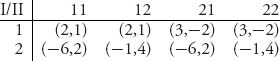
Gambit labels the strategies according to the following scheme:
![]()
A branch at a node is also called an action. Translated, 21 is the player II strategy to take action 2 (Right) at information set 1 (Up), and take action 1 (Left) at information set 2 (Down). In other words, it is strategy RL.
Simultaneous Moves. The idea now is that players I and II will choose their move at the same time, that is, without the knowledge of the opponent’s move. Each player makes a choice and they calculate the payoff. That is typically the set up we have studied in earlier chapters when we set up a matrix game. This is considering the reverse situation now—modeling simultaneous moves using a game tree. The way to model this in Gambit is illustrated in Figure 4.2.
It looks almost identical to the Figure 4.1 with sequential moves but with a crucial difference, namely, the dotted lines connecting the end nodes of player I’s choice. This dotted line groups the two nodes into an information set for player II. What that means is that player II knows only that player I has made a move landing her in information set 2: 1, but not exactly what player I’s choice has been. Player II does not know which action U or D has been chosen by I. In fact, in general, the opposing player never knows which precise node has been reached in the information set, only that it is one of the nodes in the set.
The strategies for the simultaneous move game are really simple because neither player knows what the other player has chosen and therefore cannot base her decision on what the other player has done. That means that L is a strategy for player II and R is a strategy for player II but L if Up and R if Down is not because player II cannot know whether Up or Down has been chosen by player I.
The game matrix becomes
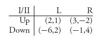
This game has a unique Nash equilibrium at (Up, L).
In general, the more information a player has, the more complicated the strategies. Simultaneous games are simpler matrix games, but more complicated extensive form games.
Given a dynamic game, we may convert to a regular matrix game by listing all the strategies for each player and calculating the outcomes when the strategies are played against each other. Conversely given the matrix form of a game we can derive the equivalent game tree as the following simple example shows.
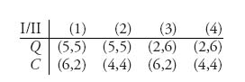
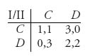
Example 4.2 Let’s consider a version of a prisoner’s dilemma game with matrix given by
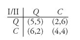
This exhibits the main feature of a prisoner’s dilemma in that the players can each do better if they keep Quiet, but since they each have an incentive to Confess they will end up at (C, C). This assumes of course that they choose without knowledge of the other player’s choice. Another way to think of it is that they choose simultaneously. Here is how to model that with a game tree (Figure 4.3).
We model this with player I making the first move, but we could just as easily pick player II as moving first since they actually choose simultaneously.
If we remove the information set at 2: 1 by making separate information sets for player II, then the game becomes a perfect information game. This would mean player I makes her choice of C or Q, and then player II makes her choice of C or Q with full knowledge of I’s choice. Now the order of play in general will make a difference (but we will see that it doesn’t in this example) (Figure 4.4).
Player I has two pure strategies: C or Q. But now player II has four pure strategies: (1) If Q, then Q; If C, then Q, (2) If Q, then Q; If C, then C, (3) If Q, then C; If C, then Q, (4) If Q, then C; If C, then C. The matrix becomes
The Nash equilibrium is still for each player to Confess. It seems that knowledge of what the other player chooses doesn’t affect the Nash equilibrium or the consequent payoffs. Is this reasonable?
Let’s think of it this way. In the case when the players choose simultaneously they have lack of information and will therefore choose (C, C). On the other hand, in the case when player I chooses first (and player II knows her choice), what would player I do? Player I would look at the payoffs at the terminal nodes and think of what player II is likely to do depending on what player I chooses. If I picks Q, then II should pick C with payoffs 2 to I and 6 to II. If I picks C, then II should also pick C with payoffs 4 to each. Since player I will then get either 2 or 4 and 4 > 2, player I should pick C. Then player II will also pick C. Player I has worked it backward with the plan of deciding what is the best thing for II to do and then picking the best thing for I to do, given that II will indeed choose the best for her. This is called backward induction and is a method for solving perfect information extensive form games. We will have much more to say about this method later.
FIGURE 4.1 Sequential moves.
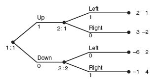
FIGURE 4.2 Simultaneous moves.
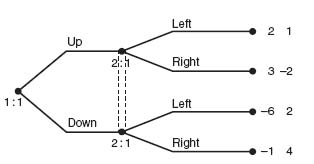
FIGURE 4.3 Prisoner’s dilemma–simultaneous choices.
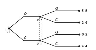
FIGURE 4.4 Prisoner’s dilemma–sequential choices.
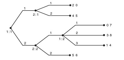
Example 4.3 Two-Stage Prisoner’s Dilemma. A natural question to ask is what happens when a game is played more than once. Suppose in a prisoner’s dilemma game each player knew that this game was going to be played again in the future. Would a suspect be so ready to rat out his accomplice if he knew the game would be played again? And would he still rat out his accomplice at each stage of the game? Does consideration of future play affect how one will play at each stage?
For example, what if we play a prisoner’s dilemma game twice. To answer that, let’s consider the two-stage extensive form of the prisoner’s dilemma given in Figure 4.5.
The information sets are designed so that each player knows her own moves but not that of the opponent. This two-stage game comes from the following one-stage game
Let’s look at the game matrix for the two-stage game using the total payoffs at the end:
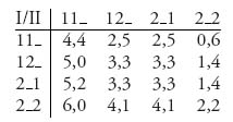
Recall that Gambit gives the strategies as the action to take at each node information set. For instance, for player II, 2_1 means at II’s first information set 2: 1, take action 2 (Don’t Confess); at the second information set 2: 2 take any action; at the third information set 2: 3, take action 1 (Confess).
The Nash equilibrium consists of I confesses in round 1, II also confesses in round 1. In round 2, they both confess. Nothing changes with this setup because there are no consequences of past actions. Everyone confesses at every round with no thought to future rounds. If the entire scope of the game is considered, however, a player should be able to decide on a strategy that uses past actions, make threats about the future, or simply reach binding agreements about future actions. This model doesn’t account for that.
One of the primary advantages of studying games in extensive form is that chance moves can easily be incorporated, as we see in the next example.
FIGURE 4.5 Two-stage prisoner's dilemma
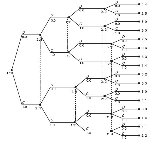
FIGURE 4.6 Russian roulette.
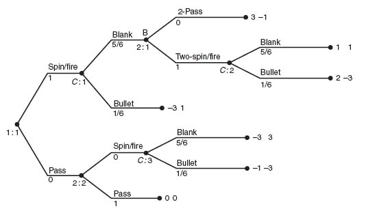
FIGURE 4.7 What are the pure strategies?
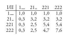
Example 4.4 Let’s consider the Russian roulette game from Chapter 1. The game tree in Gambit is shown in Figure 4.6.
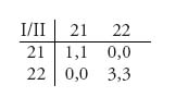
In this version of the game, player I goes first and decides whether to pass the gun or spin the chamber and fire. Recall that the gun is a six shooter and with one bullet has a ![]() chance of firing after spinning. If player I has chosen to pass, or if player I has chosen to spin/fire and lives, then the gun is passed to player II, who then has the same choices with consequent payoffs. The new feature of the game tree is that a third player, Nature, determines the outcome of the spinning. Nature provides the chance move and earns no payoff. This is an example of a perfect information game with chance moves. It is perfect information in the sense that both players can see all of the opponent’s choices, even though the outcome of the chance move is unknown before the spinning actually takes place.
chance of firing after spinning. If player I has chosen to pass, or if player I has chosen to spin/fire and lives, then the gun is passed to player II, who then has the same choices with consequent payoffs. The new feature of the game tree is that a third player, Nature, determines the outcome of the spinning. Nature provides the chance move and earns no payoff. This is an example of a perfect information game with chance moves. It is perfect information in the sense that both players can see all of the opponent’s choices, even though the outcome of the chance move is unknown before the spinning actually takes place.
The strategies for each player are fairly complicated for this game and we will not list them again but this is the matrix for the game.
Gambit produces this matrix as the equivalent strategic form of the game. Recall that the labeling of the strategies is according to the scheme ij = the ith action is taken at information set 1, the jth action is taken at info set 2. For instance, strategy 21 means player II takes action (=branch) 2 at her first info set (at 2: 1), and action 1 at her second info set (at 2: 2). In words, this translates to If I Spins (and survives), then Spin; If I Passes, then Spin.
This game has a pure Nash equilibrium given by X* = (1, 0), Y* = (0, 0, 1, 0) or Y* = (0, 0, 0, 1). The expected payoffs to each player are ![]() and
and ![]() . In the tree, the numbers below each branch represent the probability of taking that branch in a Nash equilibrium. The numbers below the chance moves represent the probability of that branch as an outcome. Note also that chance nodes are indicated with a C on the tree. That is, C: 1, C: 2, C: 3 are the information sets for Nature.
. In the tree, the numbers below each branch represent the probability of taking that branch in a Nash equilibrium. The numbers below the chance moves represent the probability of that branch as an outcome. Note also that chance nodes are indicated with a C on the tree. That is, C: 1, C: 2, C: 3 are the information sets for Nature.
Remark It is worth emphasizing that a perfect information game is a game in which every node is a separate information set. If two or more nodes are included in the same information set, then it is a game with incomplete information. The nodes comprising an information set are connected with dotted lines.
Remark Every extensive game we consider can be reduced to strategic form once we know the strategies for each player. Then we can apply all that we know about matrix games to find Nash equilibria. How do we reduce a game tree to the matrix form, that is, extensive to strategic? First, we must find all the pure strategies for each player. Remember that a pure strategy is a plan that tells the player exactly what move to make from the start to the finish of the game depending on the players knowledge of the opponent’s moves. In many, if not most extensive games, it is not feasible to list all of the pure strategies because there are too many. In that case, we must have a method of solving the game directly from the tree. If the number of pure strategies is not too large then the procedure to reduce to a strategic game is simple: play each strategy against an opposing strategy and tabulate the payoffs.
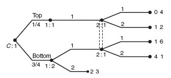
Example 4.5 Suppose we are given the following game tree with chance moves depicted in extensive form (Figure 4.7).
This game starts with a chance move. With probability ![]() player I moves to 1: 1; with probability
player I moves to 1: 1; with probability ![]() player I moves to 1: 2. From 1: 1 player I has no choices to make and it becomes player II’s turn at 2: 1. Player II then has two choices.
player I moves to 1: 2. From 1: 1 player I has no choices to make and it becomes player II’s turn at 2: 1. Player II then has two choices.
From 1: 2, player I can choose either action 1 or action 2. If action 2 is chosen the game ends with I receiving 2 and II receiving 3. If action 1 is chosen player II then has two choices, action 1 or action 2. Now since there is an information set consisting of two decision nodes for player II at 2: 1, the tree models the fact that when player II makes her move she does not know if player I has made a move from Top or from Bottom. On the other hand, because nodes at 1: 1 and 1: 2 are not connected (i.e., they are not in the same information set), player I knows whether he is at Top or Bottom. If these nodes were in the same information set, the interpretation would be that player I does not know the outcome of the chance move.
This game is not hard to convert to a matrix game. Player I has two strategies and so does player II.
Here’s where the numbers come from in the matrix. For example, if we play 11 against 1, we have the expected payoff for player II is ![]() (4) +
(4) + ![]() (6) =
(6) = ![]() . The expected payoff for player I is
. The expected payoff for player I is ![]() (0) +
(0) + ![]() (1) =
(1) = ![]() . If we play 12 against 2, the expected payoff to player II is
. If we play 12 against 2, the expected payoff to player II is ![]() (2) +
(2) + ![]() (3) =
(3) = ![]() and the expected payoff to player I is
and the expected payoff to player I is ![]() (1) +
(1) + ![]() (2) =
(2) = ![]() .
.
Our next example models and solves a classic end game situation in poker and illustrates further the use of information sets.
Example 4.6 This example illustrates again that bluffing is an integral part of optimal play in poker. For a reader who is unaware of the term bluffing, it means that a player bets on a losing card with the hope that the opponent will think the player has a card that will beat him. Anyway, here’s the model.
Two players are in a card game. A card is dealt to player I and it is either an Ace or a Two. Player I knows the card but player II does not. Player I has the choice now of either (B)etting or (F)olding. Player II, without knowing the card I has received, may either (C)all, (R)aise, or (F)old. If player II raises, then player I may either (C)all, or (F)old. The game is then over and the winner takes the pot. Initially the players ante $1 and each bet or raise adds another dollar to the pot. The tree is illustrated in Figure 4.8.
Every node is a separate information set except for the information set labeled at 2: 1 for player II. This is required since player II does not know which card player I was dealt. If instead we had created a separate information set for each node (making it a perfect information game), then it would imply that player I and II both knew the card. That isn’t poker.
Although there are many strategies for this game, most of them are dominated (strictly or weakly) and Gambit reduces the matrix to a simple 2 × 3,
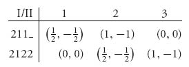
Player II has 3 strategies: (1) Call, (2) Raise, and (3) Fold. After eliminating the dominated strategies, player I has two strategies left. Here is what they mean:
This game has a Nash equilibrium leading to the payoff of ![]() to player I and −
to player I and −![]() to player II. The equilibrium tells us that if player I gets an Ace, then always Bet; player II doesn’t know if I has an Ace or a Two but II should Call with probability
to player II. The equilibrium tells us that if player I gets an Ace, then always Bet; player II doesn’t know if I has an Ace or a Two but II should Call with probability ![]() and Fold with probability
and Fold with probability ![]() . Player II should never Raise. On the other hand, if player I gets a Two, player I should Bet with probability
. Player II should never Raise. On the other hand, if player I gets a Two, player I should Bet with probability ![]() and Fold with probability
and Fold with probability ![]() ; player II (not knowing I has a Two) should Call with probability
; player II (not knowing I has a Two) should Call with probability ![]() and Fold with probability
and Fold with probability ![]() . Since player II should never Raise a player I bet, the response by player I to a Raise never arises.
. Since player II should never Raise a player I bet, the response by player I to a Raise never arises.
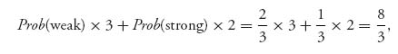
The conclusion is that player I should bluff one-third of the time with a losing card. Player II should Call the bet two-thirds of the time. The result is that, on average, player I wins ![]() .
.
Extensive games can be used to model quite complicated situations like the Greeks versus the Persians. The Greco-Persian Wars lasted from 499-449 BC. Our next example describes one fictional battle.
Example 4.7 The Persians have decided to attack a village on a Greek defended mountain. They don’t know if the Persians have decided to come by the Road to the village or Climb up the side of the mountain. The Greek force is too small to defend both possibilities. They must choose to defend either the Road to the village or the path up the side of the mountain, but not both.
But the Persians are well aware of the Greek warrior reputation for ferocity so if the Persians meet the Greeks, they will retreat. This scores one for the Greeks. If the two forces do not engage the Persians will reach a Greek arms depot and capture their heavy weapons which gives them courage to fight. If the Persians reach the arms depot the Greeks learn of it and now both sides must plan what to do as the Persians return from the arms depot. The Greeks have two choices. They can either lay an ambush on the unknown path of return or move up and attack the Persians at the arms depot. The Persians have two choices. They can either withdraw immediately by day or wait for night.
If the Persians meet an ambush by day they will be destroyed (score one for the Greeks). If the Persians meet the ambush at night they can make it through with a small loss (score one for the Persians). If the Greeks attacks the arsenal and the Persians have already gone, the Persians score one for getting away. If the Greeks attack and find the Persians waiting for night both sides suffer heavy losses and each scores zero. Assume the Greeks, having an in-depth knowledge of game theory, will assume the Persians make the first move, but this move is unknown to the Greeks.
This is a zero sum game that is most easily modeled in extensive form using Gambit.
The solution is obtained by having Gambit find the equilibrium. It is illustrated in Figure 4.9 by the probabilities below the branches. We describe it in words. The Persians should flip a fair coin to decide if they will climb the side of the mountain or take the road. Assuming the Greeks have not defended the chosen Persian route, the Persians reach the arms depot. Then they flip a three-sided coin so that with probability ![]() they will withdraw by day, and with probability
they will withdraw by day, and with probability ![]() they will wait for night.
they will wait for night.
The Greeks will flip a fair coin to decide if they will defend the road or defend the climb up the side of the mountain. Assuming they defended the wrong approach and the Persians have reached the arms depot, the Greeks will then flip a three-sided coin so that with probability ![]() they will lay an ambush and with probability
they will lay an ambush and with probability ![]() they will attack the depot hoping the Persians haven’t fled. This is a zero sum game with value +
they will attack the depot hoping the Persians haven’t fled. This is a zero sum game with value +![]() for the Greeks. If you think the payoffs to each side would make this a non zero sum game, all you have to do is change the numbers at the terminal node and resolve the game using Gambit.
for the Greeks. If you think the payoffs to each side would make this a non zero sum game, all you have to do is change the numbers at the terminal node and resolve the game using Gambit.
The next example shows that information sets can be a little tricky. You have to keep in mind what information is revealed at each node.
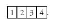
Example 4.8 A Simple Naval Warfare Game. Consider a part of the ocean as a 1 × 4 grid. The grid is
A submarine is hiding in the grid that the navy is trying to locate and destroy. Assume that the sub occupies two consecutive squares. In a search algorithm, the navy must pick a square to bomb, see if it misses or hits the sub, pick another square to bomb, and so on until the sub is destroyed. The payoff to the sub is the number of squares the navy must bomb in order to hit both parts of the sub. Assume that if a square is bombed and part of the sub is hit, the navy knows it.
The strategies for the submarine are clear: Hide in 1-2, Hide in 2-3, or Hide in 3-4. The strategies for the bomber are more complicated because of the sequential nature of the choices to bomb and the knowledge of whether a bomb hit or missed. Figure 4.10 is a Gambit depiction of the problem.
The first player is the submarine that chooses to hide in 1-2, 2-3, or 3-4. The navy bomber is player II and he is the last player to make any decisions. In each case, he decides to shoot at 1, 2, 3, or 4 for the first shot. The information set 2: 1 in Figure 4.10 indicates that the bomber does not know in which of the three pairs of squares the sub is hidden. Without that information set, player II would know exactly where the sub was and that is not a game.
Here’s an explanation of how this is analyzed referring to Figure 4.10. Let’s assume that the sub is in 1-2. The other cases are similar.
- If player II takes his first shot at 1, then it will be a hit and II knows the sub is in 1-2 so the second shot will be at 2. The game is over and the payoff to I is 2.
- If player II takes the first shot at 2, it will be a hit and the rest of the sub must be in 1 or 3. If the bomber fires at 1, the payoff will be 2; if the sub fires at 3, the payoff will be 3 because the sub will miss the second shot but then conclude the sub must be in 1-2.
- If player II takes the first shot at 3, it will be a miss. Then player II knows the sub must be in 1-2 so the payoff will be 3.
- If player II takes the first shot at 4, it will be a miss. Player II then may fire at 1, 2, or 3. If the bomber fires at 1, it will be a hit and the sub must be in 1-2, giving a payoff of 3. If the bomber fires at 3, it will be a miss. The sub must then be in 1-2 and the payoff is 4. If the bomber fires at 2, it will be a hit but the sub could be in 1-2 or 2-3. This will require another shot. The resulting payoff is either 3 or 4.
The information sets in this game are a bit tricky. First, player II, the bomber, at the first shot has the information set 2: 1 because the bomber doesn’t know which two squares the sub occupies. At the second shot, player II will know if the first shot hit or missed but cannot know more than that. Thus, information set 2: 2 means the bomber’s first shot at square 2 hit, but it is unknown if the sub is in 1-2 or 2-3. Information set 2: 3 means the first shot at 4 missed, but it is unknown if that means the sub is in 1-2 or 2-3. The rest of the information sets are similar.
After eliminating dominated strategies the game matrix reduces to
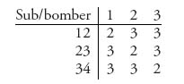
We are labeling as strategies 1, 2, 3 for the bomber.
The matrix game may be solved using the invertible matrix theorem, Mathematica, or Gambit. The value of this game is v(A) = ![]() , so it takes a little over 2 bombs, on average, to find and kill the sub. The sub should hide in 1 − 2 2 − 3, or 3 − 4 with equal probability,
, so it takes a little over 2 bombs, on average, to find and kill the sub. The sub should hide in 1 − 2 2 − 3, or 3 − 4 with equal probability, ![]() . The bomber should play strategies 1, 2, or 3, with equal probability. The strategies depend on which node player II happens to be at so we will give the description in a simple to follow plan.
. The bomber should play strategies 1, 2, or 3, with equal probability. The strategies depend on which node player II happens to be at so we will give the description in a simple to follow plan.
The bomber should fire at 2 with probability ![]() and at 3 with probability
and at 3 with probability ![]() 2 with the first shot and never fire at 1 or 4 with the first shot. If the first shot is at 2 and it is a hit, the next shot should be at 1. The game is then over because if it is a miss the bomber knows the sub is in 3-4. If the first shot is at 3 and it is a hit, the next shot should be at 2 or 4 with probability
2 with the first shot and never fire at 1 or 4 with the first shot. If the first shot is at 2 and it is a hit, the next shot should be at 1. The game is then over because if it is a miss the bomber knows the sub is in 3-4. If the first shot is at 3 and it is a hit, the next shot should be at 2 or 4 with probability ![]() , and the game is over.
, and the game is over.
FIGURE 4.8 Poker with bluffing.
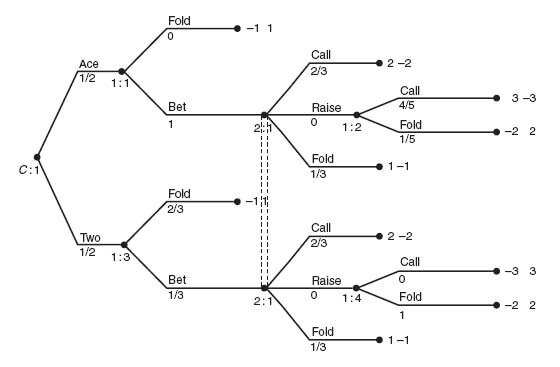
FIGURE 4.9 Battle tactics.
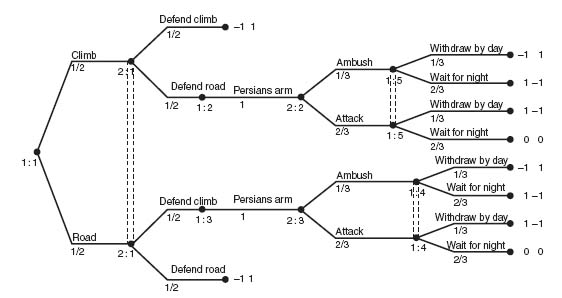
FIGURE 4.10 Submarine in 1 × 4 grid.
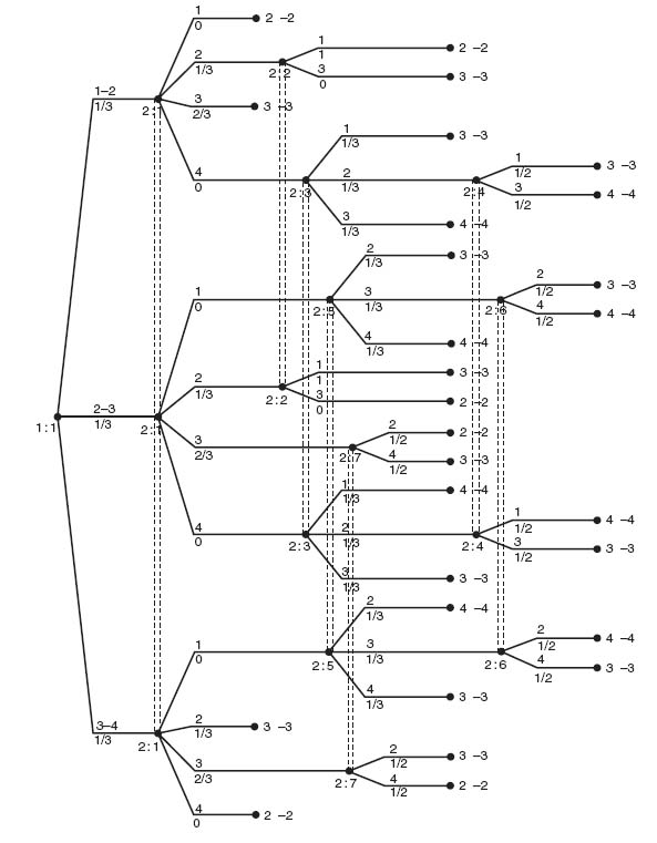
FIGURE 4.11 Game without perfect recall.
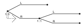
FIGURE 4.12 The full tree.
In all of these games we assume the players have perfect recall. That means each player remembers all of her moves and all her choices in the past. Here is what Gambit shows you when you have a game without perfect recall (see Figure 4.11).
This models a player who chooses initially Left or Right and then subsequently also must choose Left or Right. The start node 1: 1 and the second node also with label 1: 1 are in the same information set which means that the player has forgotten that she went Right the first time. This type of game is not considered here and you should beware of drawings like this when you solve the problems using Gambit.
Problems
4.1 Convert the following extensive form game to a strategic form game. Be sure to list all of the pure strategies for each player and then use the matrix to find the Nash equilibrium.
4.2 Given the game matrix draw the tree. Assume the players make their choices simultaneously. Solve the game.
4.3 Consider the three-player game in which each player can choose Up or Down. In matrix form the game is
4.4 In Problem 2.45, we considered the game in which Sonny is trying to rescue family members Barzini has captured. With the same description as in that problem, draw the game tree and solve the game.
4.5 Aggie and Baggie are each armed with a single coconut cream pie. Since they are the friends of Larry and Curly, naturally, instead of eating the pies they are going to throw them at each other. Aggie goes first. At 20 paces she has the option of hurling the pie at Baggie or passing. Baggie then has the same choices at 20 paces but if Aggie hurls her pie and misses, the game is over because Aggie has no more pies. The game could go into a second round but now at 10 paces, and then a third round at 0 paces. Aggie and Baggie have the same probability of hitting the target at each stage: ![]() at 20 paces,
at 20 paces, ![]() at 10 paces, and 1 at 0 paces. If Baggie gets a pie in the face, Aggie scores +1, and if Aggie gets a pie in the face Baggie scores +1. This is a zero sum game.
at 10 paces, and 1 at 0 paces. If Baggie gets a pie in the face, Aggie scores +1, and if Aggie gets a pie in the face Baggie scores +1. This is a zero sum game.
4.6 One possibility not accounted for in a Battle of the Sexes game is the choice of player I to go to a bar instead of the Ballet or Wrestling. Suppose the husband, who wants to go to Wrestling, has a 15% chance of going to a bar instead. His wife, who wants to go to the Ballet, also has a 25% chance of going to the same bar instead. If they both meet at Wrestling, the husband gets 4, the wife gets 2. If they both meet at the Ballet, the wife gets 4, and the husband gets 1. If they both meet at the bar, the husband gets 4 and the wife also gets 4. If they decide to go to different places they each get 2. Assume the players make their decisions without knowledge of the other’s choice. Draw the game and solve using Gambit.
4.2 Backward Induction and Subgame Perfect Equilibrium
Backward induction is a simple way to solve a game with perfect information and perfect recall. It is based on the simple idea that the players will start at the end of the tree, look at the payoffs, choose the action giving them the largest payoff, and work backward to the beginning of the game. This has obvious limitations we will go over. But first let’s look at an example.
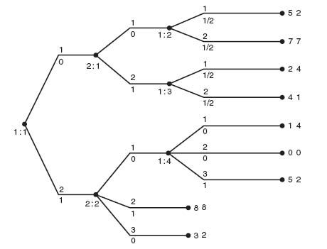
Example 4.9 This is a two-player game with perfect information and perfect recall. To find the equilibrium given by backward induction we start at the end and look at the payoffs to the last player to choose a branch (Figure 4.12).
In this case, player I makes the last choice. For the node at 1: 2, player I would clearly choose branch 2 with payoff (7, 7). For the node at 1: 3, player I would choose branch 2 with payoff (4, 1). Finally, for the node at 1: 4, player I would choose branch 3 with payoff (5, 2). Eliminate all the terminal branches player I would not choose. The result is shown in Figure 4.13.
Now we work backward to player 2’s nodes using Figure 4.13. At 2: 1 player 2 would choose branch 1 since that gives payoff (7, 7). At 2: 2, player 2 chooses branch 2 with payoff (8, 8). Eliminating all other branches gives us the final game tree (Figure 4.14).
Using Figure 4.14, working back to the start node 1: 1, we see that player 1 would choose branch 2, resulting in payoff (8, 8). We have found an equilibrium by backward induction. The backward induction equilibrium is that player 1 chooses branch 2 and player 2 chooses branch 2. Gambit solves the game and gives three Nash equilibria including the backward induction one. The other two equilibria give a lower payoff to each player, but they are equilibria.
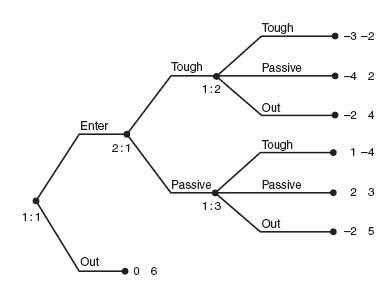
Example 4.10 We will see in this example that backward induction picks out the reasonable Nash equilibrium. Suppose there are two firms A and B that produce competing widgets. Firm A is thinking of entering a market in which B is the only seller of widgets. A game tree for this model is shown in Figure 4.15.
The matrix for this game is
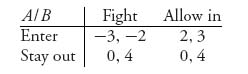
There are two pure Nash equilibria at (0, 4) and (2, 3) corresponding to (Stay out, Fight) and (Enter, Allow in), respectively. Now something just doesn’t make sense with the Nash equilibrium (Stay out, Fight). Why would firm B Fight, when firm A Stays out of the market? That Nash equilibrium is just not credible.
Now let’s see which Nash equilibrium we get from backward induction. The last move chosen by B will be Allow in from node 2: 1. Then A, knowing B will play Allow in will choose Enter since that will give A a larger payoff. Thus, the Nash equilibrium determined by backward induction is (Enter, Allow in) resulting in payoff (2, 3). The incredible Nash equilibrium at (0, 4) is not picked up by backward induction.
A more complicated example gives an application to conflicts with more options.
Example 4.11 Solomon’s Decision. A biblical story has two women before King Solomon in a court case. Both women are claiming that a child is theirs. Solomon decides that he will cut the child in half and give one half to each woman. Horrified, one of the women offers to give up her claim to the kid so that the child is not cut in two. Solomon awards the child to the woman willing to give up her claim, deciding that she is the true mother. This game (due to Herve Moulin3) gives another way to decide who is the true mother without threatening to cut up the child.
Solomon knows that one of the women is lying but not which one, but the women know who is lying. Solomon assumes the child is worth CT to the real mother and worth CF to the false mother, with CT > > CF. In order to decide who is the true mother Solomon makes the women play the following game:
To begin, woman 1 announces Mine or Hers. If she announces Hers, woman 2 gets the child and the game is over. If she announces Mine, woman 2 either Agrees or Objects. If woman 2 Agrees, then woman 1 gets the child and the game is over. If woman 2 Objects, then woman 2 pays a penalty of $V where CF < V < CT, but she does get the child, and woman 1 pays a penalty of $W > 0.
We will consider two cases to analyze this game. In the analysis we make no decision based on the actual values of CT, CF, which are unknown to Solomon.
Case 1: Woman 1 is the true mother. The tree when woman 1 is the true mother is shown in Figure 4.16.
In view of the fact that CF − V < 0, we see that woman 2 will always choose to Agree, if woman 1 chooses Mine. Eliminating the Object branch, we now compare the payoffs (CT, 0) with (0, CF) for woman 1. Since CT > 0, woman 1 will always call Mine. By backward induction we have the equilibrium that woman 1 should call Mine, and woman 2 should Agree. The result is that woman 1, the true mother, ends up with the child.
Case 2: Woman 2 is the true mother. The tree when woman 2 is the true mother is shown in Figure 4.17.
Now we have CT − V > 0, and woman 2 will always choose to Object, if woman 1 chooses Mine. Eliminating the Agree branch, we now compare the payoffs (−W, CT − V) with (0, CT) for woman 1. Since −W < 0, woman 1 will always call Hers. By backward induction, we have the equilibrium that woman 1 should call Hers, and woman 2 should Object if woman 1 calls Mine. The result is that woman 2, the true mother, ends up with the child. Thus, by imposing penalties and assuming that each woman wants to maximize her payoff, King Solomon's decision does not involve infanticide.
Problems
4.7 Modify Solomon’s decision problem so that each woman actually loses the value she places on the child if she is not awarded the child. The value to the true mother is assumed to satisfy CT>2CF. Assume that Solomon knows both CT and CF and so can set V > 2 CF. Apply backward induction to find the Nash equilibrium and verify that the true mother always gets the child.
4.8 Find the Nash equilibrium using backward induction for the tree:
4.9 Two players ante $1. Player I is dealt an Ace or a Two with equal probability. Player I sees the card but player II does not. Player I can now decide to Raise, or Fold. If he Folds, then player II wins the pot if the card is a Two, while player I wins the pot if the card is an Ace. If player I Raises, he must add either $1 or $2 to the pot. Player II now decides to Call or Fold. If she Calls and the card was a Two, then II wins the pot. If the card was an Ace, I wins the pot. If she Folds, player I takes the pot. Model this as an extensive game and solve it using Gambit.
4.2.1 SUBGAME PERFECT EQUILIBRIUM
An extensive form, game may have lots of Nash equilibria and often the problem is to decide which of these, if any, are actually useful, implementable, or practical. Backward induction, which we considered in the previous section was a way to pick out a good equilibrium. The concept of subgame perfection is a way to eliminate or pick out certain Nash equilibria which are the most implementable. The idea is that at any fixed node, a player must make a decision which is optimal from that point on. In fact, it makes sense that a player will choose to play according to a Nash equilibrium no matter at which stage of the game the player finds herself, because there is nothing that can be done about the past. A good Nash equilibrium for a player is one which is a Nash equilibrium for every subgame. That is essentially the definition of subgame perfect equilibrium.
We assume that our game has perfect recall. Each player remembers all her past moves. In particular, this means that an information set cannot be split into separate nodes. For instance, in the following game in Figure 4.18 below there are no proper subgames. This is a game in which player I holds an Ace or a Two. Player II without knowing which card player I holds, guesses that I holds an Ace or I holds a Two. If player II is correct, II wins $1, and loses $1 if incorrect.
FIGURE 4.13 The reduced tree.
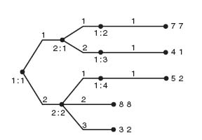
FIGURE 4.14 The final reduction.
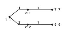
FIGURE 4.15 Entry deterrence.
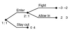
FIGURE 4.16 Woman 1 is the true mother.
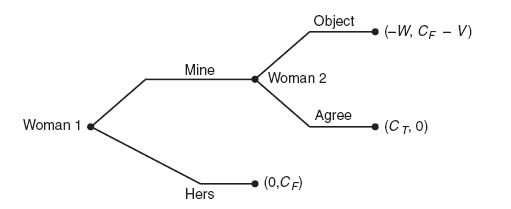
FIGURE 4.17 Woman 2 the true mother.
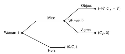
FIGURE 4.18 An extensive game with no proper subgames.
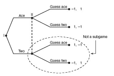
FIGURE 4.19 Up-Down-Left-Right.
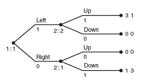
FIGURE 4.20 Subgame perefect equilibrium.
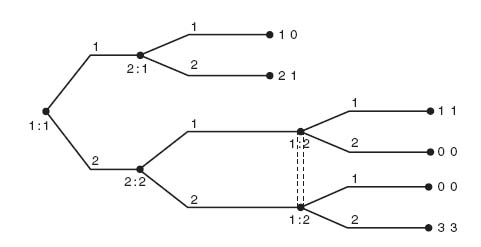
FIGURE 4.21 Two-stage russian roulette.
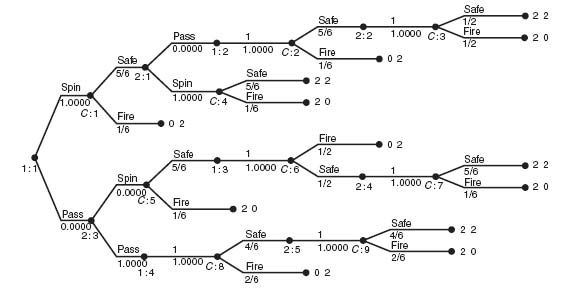
FIGURE 4.22 The first reduction.
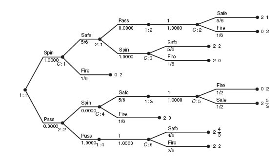
FIGURE 4.23 The second reduction.
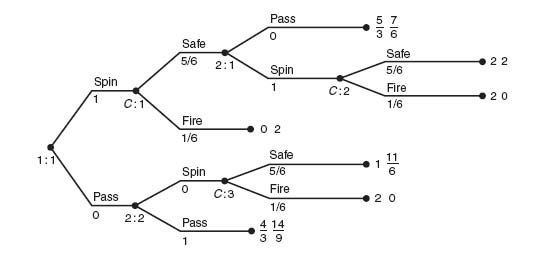
FIGURE 4.24 The last reduction.
FIGURE 4.25 Gale’s roulette.
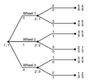
FIGURE 4.26 Gale’s roulette with high number payoff.
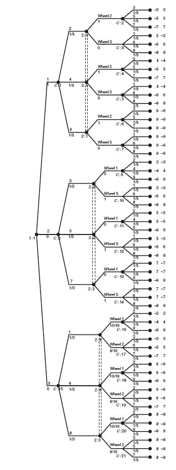
FIGURE 4.27 Six-stage centipede game.
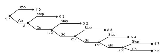
FIGURE 4.28 Beer or quiche signalling game.
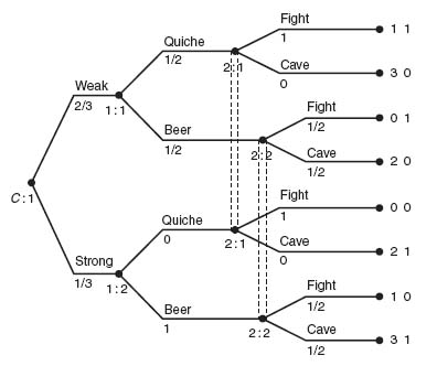
FIGURE 4.29 Prisoner's dilemma with a conscience.
Now here is the precise definition.
Definition 4.2.1 A subgame perfect equilibrium for an extensive form game is a Nash equilibrium whose restriction to any subgame is also a Nash equilibrium of this subgame.
Example 4.12 We return to the Up-Down-Left-Right game given in Figure 4.19.
There are two subgames in this game but only player II moves in the subgames. The game has three pure Nash equilibria:
Which of these, if any are subgame perfect? Start at player II’s moves. If I chooses Left, then II clearly must choose Up since otherwise II gets 0. If I chooses Right, then II must choose Down. This means that for each subgame, the equilibrium is that player II chooses Up in the top subgame and Down in the bottom subgame. Thus, strategy (3) is subgame perfect; (1) and (2) are not.
You may have noticed the similarity in finding the subgame perfect equilibrium and using backward induction. Directly from the definition of subgame perfect, we know that any Nash equilibrium found by backward induction must be subgame perfect. The reason is because backward induction uses a Nash equilibrium from the end of the tree to the beginning. That means it has to be subgame perfect. This gives us a general rule: To find a subgame perfect equilibrium use backward induction.
How do we know, in general, that a game with multiple Nash equilibria, one of them must be subgame perfect? The next theorem guarantees it.
Theorem 4.2.2 Any finite tree game in extensive form has at least one subgame perfect equilibrium.
Proof. We use induction on the number of proper subgames.
Suppose first the game has no proper subgames. In this case, since the game definitely has a Nash equilibrium, any Nash equilibrium must be subgame perfect.
Now, suppose we have a game with a proper subgame but which has no proper subgames of its own. This subgame has at least one Nash equilibrium and this equilibrium gives each player a payoff of the subgame. Now replace the entire subgame with a new Terminal node with this subgame’s payoffs.
Therefore, we now have a game which has one less proper subgames than the original game. By the induction hypothesis, this new game has a subgame perfect equilibrium.
Next, take the subgame perfect equilibrium just found and add the Nash equilibrium of the subgame we found in the first step. This tells each player what to do if the Terminal node is reached. Now it is a matter of checking that the equilibrium constructed in this way is subgame perfect for the original game. That is an easy exercise. ![]()
We can say more about subgame perfect equilibria if the game has perfect information (each node has its own information set).
Theorem 4.2.3 (1) Any finite game in extensive form with perfect information has at least one subgame perfect equilibrium in pure strategies.
(2) Suppose all payoffs at all terminal nodes are distinct for any player. Then there is one and only one subgame perfect equilibrium.
(3) If a game has no proper subgames, then every Nash equilibrium is subgame perfect.
The proof of this theorem is by construction because a subgame perfect equilibrium in pure strategies can be found by backward induction. Just start at the end and work backward as we did earlier. If all the payoffs are distinct for each player then this will result in a unique path back through the tree.
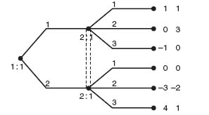
Example 4.13 In the following tree, there are three subgames: (1) the whole tree, (2) the game from node 2: 1, and (3) the game from node 2: 2. The subtree from information set 1: 2 does not constitute two more subgames because that would slice up an information set (Figure 4.20).
The equivalent strategic form of the game is
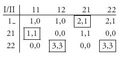
This game has four pure Nash equilibria shown as boxed in the matrix. Now we seek the subgame perfect equilibrium.
Begin by solving the subgame starting from 2: 2. This subgame corresponds to rows 2 and 3, and columns 3 and 4 in the matrix for the entire game. In other words, the subgame matrix is
This subgame has three Nash equilibria resulting in payoffs (3, 3), (![]() ,
, ![]() ), (1, 1).
), (1, 1).
Next, we consider the subgame starting from 1: 1 with the subgame from 2: 2 replaced by the payoffs previously calculated. Think of 2: 2 as a terminal node.
With payoff (1, 1) (at node 2: 2) we solve by backward induction. Player II will use action 2 from 2: 1. Player I chooses action 1 from 1: 1. The equilibrium payoffs are (2, 1). Thus, a subgame perfect equilibrium consists of player I always taking branch 1, and player II always using branch 2 from 2: 1.
With payoff (![]() ,
, ![]() ) at node 2: 2, the subgame perfect equilibrium is the same.
) at node 2: 2, the subgame perfect equilibrium is the same.
With payoff (3, 3) at node 2: 2, Player II will choose action 2 from 2: 1. Player I always chooses action 2 from 1: 1. The equilibrium payoffs are (3, 3) and this is the subgame perfect equilibrium.
This game does not have a unique subgame perfect equilibrium since the subgame perfect equilibria are the strategies giving the payoffs (3, 3) and (2, 1). But we have eliminated the Nash equilibrium giving (1, 1).
Example 4.14 This example will indicate how to use Gambit to find subgame perfect equilibria for more complex games. Suppose we consider a two-stage game of Russian roulette. Player I begins by making the choice of spinning and firing or passing. The gun is a six shooter with one bullet in the chambers. If player I passes, or survives, then player II has the same two choices. If a player doesn’t make it in round 1, the survivor gets 2 and the loser gets 0.
In round 2 (if there is a round 2) if both players passed in round 1, the gun gets an additional bullet and there is no option to pass. If player I passed and player II spun in round 1, then in round 2 player I must spin and the gun now has 3 bullets. If player I survives that, then player II must spin but the gun has 1 bullet.
If player I spun in round 1 and player II passed, then in the second round player I must spin with 1 bullet. If player I is safe, then player II must spin with 3 bullets. In all cases, a survivor gets 2 and a loser gets 0.
The game tree using Gambit is shown in Figure 4.21.
Gambit gives us the Nash equilibrium that in round 1 player I should spin. If I survives, II should also spin. The expected payoff to player I is 1.667 and the expected payoff to player II is 1.722. Is this a subgame perfect equilibrium? Let’s use backward induction to find the Nash.
Gambit has the very useful feature that if we click on a node it will tells us what the node value is. The node value to each player is the payoff to the player if that node is reached. If we click on the nodes 2: 2, 2: 4, and 2: 5, we get the payoffs to each player if those nodes are reached. Then we delete the subtrees from those nodes and specify the payoffs at the node as the node values for each player. The resulting tree is shown in Figure 4.22.
In this tree player I makes the last move but he has no choices to make.
Now let’s move back a level by deleting the subtrees from 1: 2, 1: 3, and 1: 4. The result is shown in Figure 4.23.
Player II should spin if player I spins and survives because his expected payoff is ![]() × 2 >
× 2 > ![]() . If player I passes, player II should also pass because
. If player I passes, player II should also pass because ![]() ×
× ![]() <
< ![]() .
.
Finally, replacing the subtrees at 2: 1 and 2: 2, we get the result that is shown in Figure 4.24.
In this last tree, player I should clearly spin, because his expected payoff is ![]() × 2 +
× 2 + ![]() × 0 =
× 0 = ![]() = 1.66 if he spins, while it is
= 1.66 if he spins, while it is ![]() = 1.33 if he passes. We have found the subgame perfect equilibrium:
= 1.33 if he passes. We have found the subgame perfect equilibrium:
This is the Nash equilibrium Gambit gave us at the beginning. Since it is actually the unique Nash equilibirum and we know a game of this type must have at least one subgame perfect equilibrium, it had to be subgame perfect, as we verified.
Incidentally, if we take half of the expected payoffs to each player we will find the probability a player survives the game. Directly, we calculate
and
Naturally, player II has a slightly better chance of surviving because player I could die with the first shot.
In the next section, we will consider some examples of modeling games and finding subgame perfect equilibria.
4.2.2 EXAMPLES OF EXTENSIVE GAMES USING GAMBIT
Many extensive form games are much too complex to solve by hand. Even determining the strategic game from the game tree can be a formidable job. In this subsection, we illustrate the use of Gambit to solve some interesting games.
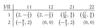
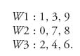
Example 4.15 Gale’s Roulette. There are two players and three wheels. The numbers on wheel 1 are 1, 3, 9; on wheel 2 are 0, 7, 8; and on wheel 3 are 2, 4, 6. When spun, each of the numbers on the wheel are equally likely. Player I chooses a wheel and spins it. While the wheel player I has chosen is still spinning, player II chooses one of the two remaining wheels and spins it. The winner is the player whose wheel stops on a higher number and the winner receives $1 from the loser. To summarize, the numbers on the wheels are
We first suppose that I has chosen wheel 1 and II has chosen wheel 2. We will find the chances player I wins the game.
Let X1 be the number that comes up from wheel 1 and X2 the number from wheel 2. Then,
Similarly, if Z3 is the number that comes up on wheel 3, then if player II chooses wheel 3 the probability player I wins is
Finally, if player I chooses wheel 2 and player II chooses wheel 3 we have
Next, we may draw the extensive form of the game and use Gambit to solve it (see Figure 4.25). Note that this is a perfect information game. The payoffs are calculated as $1 times the probability of winning to player I and $1 times the probability of winning for player II.
Gambit gives us four Nash equilibria all with the payoffs ![]() to player I and
to player I and ![]() to player II. There are two subgame perfect Nash equilibria. The first equilibrium consists of player I always choosing wheel 2 and player II subsequently choosing wheel 1. The second subgame perfect equilibrium is player I chooses wheel 1 and player II subsequently chooses wheel 3. Both of these are constructed using backward induction. The expected winnings for player I is 1 ·
to player II. There are two subgame perfect Nash equilibria. The first equilibrium consists of player I always choosing wheel 2 and player II subsequently choosing wheel 1. The second subgame perfect equilibrium is player I chooses wheel 1 and player II subsequently chooses wheel 3. Both of these are constructed using backward induction. The expected winnings for player I is 1 · ![]() − 1 ·
− 1 · ![]() = −
= − ![]() .
.
This problem is a little more interesting if we change the payoff to the following rule: If the high number on the winning wheel is N, then the loser pays the winner $N. We could analyze this game using probability. In the interest of showing how Gambit can be used to conceptually simplify the problem, let’s draw the tree (see Figure 4.26).
In this example, we need no knowledge of probability or how to calculate the expected payoffs. Interestingly enough, the value of this zero sum game is v = ![]() . The optimal strategies are player I always chooses wheel 1, and player II always chooses wheel 2. The game matrix is
. The optimal strategies are player I always chooses wheel 1, and player II always chooses wheel 2. The game matrix is
It is easy to check that the numbers in the matrix are the actual expected payoffs. For instance, if player I uses wheel 1 and player II chooses wheel 2, the expected payoff is (− 3 − 5 − 7 + 4 − 5 − 7 + 9 + 9 + 9)/9 = ![]() .
.
Our next example has been studied by many economists and is a cornerstone of the field of behavioral economics and political science which tries to predict and explain irrational behavior.
Example 4.16 This game is commonly known as the centipede game because of the way the tree looks. The game is a perfect information, perfect recall game. Each player has two options at each stage, Stop, or Continue. Player I chooses first so that player I chooses in odd stages 1, 3, 5, …. Player II chooses in even numbered stages 2, 4, 6, ….
The game begins with player I having 1 and player II having 0. In round 1, player I can either Stop the game and receive her portion of the pot, or give up 1 and Go in the hope of receiving more later. If player I chooses Go, player II receives an additional 3. In each even round player II has the same choices of Stop or Go. If II chooses Go her payoff is reduced by 1 but player I’s payoff is increased by 3. The game ends at round 100 or as soon as one of the players chooses Stop.
We aren’t going to go 100 rounds but we can go 6. The extensive game is shown in Figure 4.27.
Gambit can solve this game pretty quickly, but we will do so by hand. Before we begin, it is useful to see the equivalent matrix form for the strategic game. Gambit gives us the matrix
In the notation for the pure strategies for player I, for example 1– means take action 1 (stop) at node 1: 1 (after that it doesn’t matter), and 221 means take action 2 (go) at 1: 1, then take action 2 (go) at 1: 2, and take action 1 (stop) at 1: 3. Immediately, we can see that we may drop column 4 since every second number in the pair is smaller (or equal) to the corresponding number in column 3. Here’s how the dominance works:
We are left with a unique Nash equilibrium at row 1, column 1, which corresponds to player I stops the game at stage 1.
Now we work this out using backward induction. Starting at the end of the tree, the best response for player II is Stop. Knowing that, the best response in stage 5 for player I is Stop, and so on back to stage 1. The unique subgame perfect equilibrium is Stop as soon as each player gets a chance to play.
It is interesting that Gambit gives us this solution as well, but Gambit also tells us that if at stage 1 player I plays Go instead of Stop, then player II should Stop with probability ![]() and Go with probability
and Go with probability ![]() at the second and each remaining even stage. Player I should play Stop with probability
at the second and each remaining even stage. Player I should play Stop with probability ![]() and Go with probability
and Go with probability ![]() at each remaining odd stage.
at each remaining odd stage.
Does the Nash equilibrium predict outcomes in a centipede game? The answer is No. Experiments have shown that only rarely do players follow the Nash equilibrium. It was also rare that players always played Go to get the largest possible payoff. In the six-stage game, the vast majority of players stopped after three or four rounds.
What could be the reasons for actually observing irrational behavior? One possibility is that players actually have some degree of altruism so that they actually care about the payoff of their opponent. Of course, it is also possible that some selfish players anticipate that their opponents are altruists and so continue the game. These hypotheses can and are tested by behavioral economists.
Our next example illustrates the modeling of signals as an imperfect information game. It is also an example of what’s called a Bayesian game because of the use of conditional probabilities.
Example 4.17 This is a classic example called the Beer or Quiche game. Curly4 is at a diner having breakfast and in walks Moe. We all know Moe is a bully and he decides he wants to have some fun by bullying Curly out of his breakfast. But we also know that Moe is a coward so he plays his tricks only on those he considers wimps. Moe doesn’t know whether Curly is a wimp or will fight (because if there is even a hint of limburger cheese, Curly is a beast) but he estimates that about ![]() of men eating breakfast at this diner will fight and
of men eating breakfast at this diner will fight and ![]() will cave.
will cave.
Moe decides to base his decision about Curly on what Curly is having for breakfast. If Curly is having a quiche, Moe thinks Curly definitely is a wimp. On the other hand, if Curly is having a beer for breakfast, then Moe assumes Curly is not a wimp and will fight. Curly knows if he is a wimp, but Moe doesn’t, and both fighters and wimps could order either quiche or beer for breakfast so the signal is not foolproof. Also, wimps sometimes choose to fight and don’t always cave.
Curly gets to choose what he has for breakfast and Moe gets to choose if he will fight Curly or cave. Curly will get 2 points if Moe caves and an additional 1 point for not having to eat something he doesn’t really want. Moe gets 1 point for correctly guessing Curly’s status. Finally, if Curly is tough, he really doesn’t like quiche but he may order it to send a confusing signal.
The game tree is shown in Figure 4.28.
Note that there are no strict subgames of this game since any subgame would cut through an information set, and hence, every Nash equilibrium is subgame perfect. Let’s first consider the equivalent strategic form of this game. The game matrix is

The labels for the strategies correspond to the labels given in the game tree. In this example, strategy 11 for player I means to take action 1 (quiche) if player I is weak and action 1 (quiche) if player I is strong. Strategy 12 means to play action 1 (quiche) at if at 1: 1 (weak) and action 2 (beer) if at 1: 2 (strong). For player II, strategy 22 means play cave (action 2) if I plays quiche (info set 2: 1) and play cave (action 2) if I plays beer (info set 2: 2).
As an example to see how the numbers arise in the matrix let’s calculate the payoff if Curly plays 11 and Moe plays 21. Curly orders Quiche whether he is strong or weak. Moe caves if he spots a Quiche but fights if he spots Curly with a Beer. The expected payoff to Curly is
and the payoff to Moe is
It is easy to check that row 3 and column 4 may be dropped because of dominance. The resulting 3 × 3 matrix can be solved using equality of payoffs as in Chapter 2. We get X* = (0, ![]() , 0,
, 0, ![]() ), Y* = (
), Y* = (![]() ,
, ![]() , 0, 0). Curly should play strategy 12 and strategy 22 with probability
, 0, 0). Curly should play strategy 12 and strategy 22 with probability ![]() , while Moe should play strategy 11 and strategy 12 with probability
, while Moe should play strategy 11 and strategy 12 with probability ![]() . In words, given that Curly is weak, he should order quiche with probability
. In words, given that Curly is weak, he should order quiche with probability ![]() and beer with probability
and beer with probability ![]() , and then Moe should fight if he sees the quiche but only fight with probability
, and then Moe should fight if he sees the quiche but only fight with probability ![]() if he sees the beer. Given that Curly is strong, Curly should always order beer, and then Moe should fight with probability
if he sees the beer. Given that Curly is strong, Curly should always order beer, and then Moe should fight with probability ![]() . Of course, Moe doesn’t know if Curly is weak or strong but he does know there is only a
. Of course, Moe doesn’t know if Curly is weak or strong but he does know there is only a ![]() chance he is strong. The payoffs are
chance he is strong. The payoffs are ![]() to Curly and
to Curly and ![]() to Moe.
to Moe.
Informally, a Bayesian game is a game in which a player has a particular characteristic, or is a particular type, with some probability, like weak or strong in the Beer-Quiche game. Practically, this means that in Gambit we have to account for the characteristic with a chance move. This is a very useful modeling technique. The next example further illustrates this.
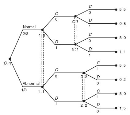
Example 4.18 A prisoner’s dilemma game in which one of the players has a conscience can be set up as a Bayesian game if the other player doesn’t know about the conscience. For example, under normal circumstances the game matrix is given by
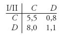
On the other hand, if player II develops a conscience the game matrix is
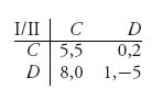
Let’s call the first game the game that is played if player II is Normal, while the second game is played if II is Abnormal. Player I does not know ahead of time which game will be played when she is picked up by the cops, but let’s say she believes the game is Normal with probability 0 < p < 1 and Abnormal with probability 1 − p. In this example, we take p = ![]() .
.
We can solve this game by using the Chance player who chooses at the start of the game which matrix will be used. In other words, the Chance player determines if player II is a type who has a conscience or not. Player II knows if they have a conscience, but player I does not. As an extensive game we model this with an information set in which player I does not know how the probability came out (see Figure 4.29).
The equivalent strategic form of the game is
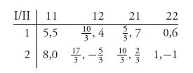
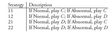
Since player I only makes a decision once at the start of the game, player I has only the two strategies 1 = C and 2 = D. For player II, we have the four strategies:
From the strategic form for the game we see immediately that for player I strategy 2 (i.e., D) dominates strategy 1 and player I will always play C. Once that is determined we see that strategy 21 dominates all the others and player II will play D, if the game is normal, but play C if the game is Abnormal. That is the Nash equilibrium for this game.
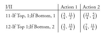
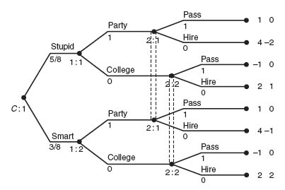
Here is an example in which the observations are used to infer a players type. Even though the game is similar to the Conscience game, it has a crucial difference through the infor-mation sets.
Example 4.19 Suppose a population has two types of people, Smart and Stupid. Any person (Smart or Stupid) wanting to enter the job market has two options, get educated by going to College, or Party. A potential employer can observe a potential employee’s educational level, but not if the potential employee is Smart or Stupid. Naturally, the employer has the decision to hire (H) or pass over (P) an applicant. We assume that there is a ![]() chance the student is Stupid and a
chance the student is Stupid and a ![]() chance the student is Smart.
chance the student is Smart.
The strategic form of this game is given by
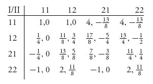
Strategies 11, 21, and 22 for player II are dominated by strategy 12; then strategy 22 for player I dominates the others. Player I, the student, should always play 22 and player II (the employer) should always play 12. Thus, the pure Nash equilibrium is X = (0, 0, 0, 1), Y =(0, 1, 0, 0). What does this translate to? Pure strategy 22 for player I (the student) means that at the first info set (i.e., at 1: 1), the student should take action 2 (college), and at the second info set (i.e, at 1: 2), the student should take action 2 (college). The Nash equilibrium 12 for player II says that at info set 2: 1 (i.e., when student chooses party), action 1 should be taken (Pass); at info set 2: 2 (student chooses college), the employer should take action 2 (Hire).
There are actually four Nash equilibria for this game:
We have seen that (X1, Y1) is the dominant equilibrium but there are others. For example X4, Y4 says that the student should always Party, whether he is Smart or Stupid, and the employer should always Pass. This leads to payoffs of 1 for the student and 0 for the employer. (This is the Nash depicted in the Figure 4.30.)
In summary, the employer will hire a college graduate and always pass on hiring a partier.
FIGURE 4.30 Party or College?
Problems
4.10 Consider the following game in extensive form depicted in the figure
4.11 BAT (British American Tobacco) is thinking of entering a market to sell cigarettes currently dominated by PM (Phillip Morris). PM knows about this and can choose to either be passive and give up market share, or be tough and try to prevent BAT from gaining any market share. BAT knows that PM can do this and then must make a decision of whether to fight back, enter the market but act passively, or just stay out entirely. Here is the tree:
Find the subgame perfect Nash equilibrium.
4.12 In a certain card game, player 1 holds two Kings and one Ace. He discards one card, lays the other two face down on the table, and announces either 2 Kings or Ace King. Ace King is a better hand than 2 Kings. Player 2 must either Fold or Bet on player 1’s announcement. The hand is then shown and the payoffs are as follows:
4.13 Solve the Beer or Quiche game assuming Curly has probability ![]() of being weak and probability
of being weak and probability ![]() of being strong.
of being strong.
4.14 Curly has two safes, one at home and one at the office.5 The safe at home is a piece of cake to crack and any thief can get into it. The safe at the office is hard to crack and a thief has only a 15% chance of getting at the gold if it is at the office. Curly has to decide where to place his gold bar (worth 1). On the other hand, the thief has a 50% chance of getting caught if he tries to hit the office and a 20% chance if he hits the house. If he gets the gold he wins 1; if he gets caught he not only doesn’t get the gold but he goes to the joint (worth −2). Find the Nash equilibrium and expected payoffs to each player.
4.15 Jack and Jill are commodities traders who go to a bar after the market closes. They are trying to determine who will buy the next round of drinks. Jack has caught a fly, and he also has a realistic fake fly. Jill, who is always prepared has a fly swatter. They are going to play the following game. Jack places either the real or fake fly on the table covered by his hand. When Jack says “ready, ” he uncovers the fly (fake or real) and as he does so Jill can either swat the fly or pass. If Jill swats the real fly, Jack buys the drinks; if she swats the fake fly, Jill buys the drinks. If Jill thinks the real fly is the fake and she passes on the real fly, the fly flies away, the game is over, and Jack and Jill split the round of drinks. If Jill passes on the fake fly, then they will give it another go. If in the second round Jill again passes on the fake fly, then Jack buys the round and the game is over. A round of drinks costs $2.
4.16 Two opposing navys (French and British) are offshore an island while the admirals are deciding whether or not to attack. Each navy is either strong or weak with equal probability. The status of their own navy is known to the admiral but not to the admiral of the opposing navy. A navy captures the island if it either attacks while the opponent does not attack, or if it attacks as strong while the opponent is weak. If the navys attack and they are of equal strength, then neither captures the island.
The island is worth 8 if captured. The cost of fighting is 3 if it is strong and 6 if it is weak. There is no cost of attacking if the opponent does not attack and there is no cost if no attack takes place. What should the admirals do?
4.17 Solve the six-stage centipede game by finding a correlated equilibrium. Since the objective function is the sum of the expected payoffs, this would be the solution assuming that each player cares about the total, not the individual. Use Maple/Mathematica for this solution.
4.18 There are three gunfighters A, B, C. Each player has 1 bullet and they will fire in the sequence A then B then C, assuming the gunfighter whose turn comes up is still alive. The game ends after all three players have had a shot. If a player survives, that player gets 2, while if the player is killed, the payoff to that player is −1.
4.19 Moe, Larry, and Curly are in a two round truel. In round 1, Larry fires first, then Moe, then Curly. Each stooge gets one shot in round 1. Each stooge can choose to fire at one of the other players, or to deliberately miss by firing in the air. In round 2, all survivors are given a second shot, in the same order of play.
Suppose Larry’s accuracy is 30%, Moe’s is 80%, and Curly’s is 100%. For each player, the preferred outcome is to be the only survivor, next is to be one of two survivors, next is the outcome of no deaths, and the worst outcome is that you get killed. Assume an accurate shot results in death of the one shot at. Who should each player shoot at and find the probabilities of survival under the Nash equilibrium.
4.20 Two players will play a Battle of the Sexes game with bimatrix
Before the game is played player I has the option of burning $1 with the result that it would drop I’s payoff by 1 in every circumstance.
4.21 There are two players involved in a two-step centipede game. Each player may be either rational (with probability ![]() ) or an Altruist (with probability
) or an Altruist (with probability ![]() ). Neither player knows the other players type.
). Neither player knows the other players type.
If both players are rational, each player may either Take the payoff or Pass. Player I moves first and if he Takes, then the payoff is 0.8 to I and 0.2 to II. If I Passes, then II may either Take or Pass. If II Takes, the payoff is 0.4 to I and 1.60 to II. If II Passes the next round begins. Player I may Take or Pass (payoffs 3.20, 0.80 if I Takes) then II may Take or Pass (payoffs 1.60, 6.40 if II Takes and 12.80, 3.20 if II Passes). The game ends.
If player I is rational and player II is altruistic, then player II will Pass at both steps. The payoffs to each player are the same as before if I Takes, or the game is at an end.
The game is symmetric if player II is rational and player I is altruistic.
If both players are altruistic then they each Pass at each stage and the payoffs are 12.80, 3.20 at the end of the second step.
Draw the extensive form of this game and find as many Nash equilibria as you can. Compare the result with the game in which both players are rational.
Bibliographic Notes
Extensive games are a major generalization of static games. Without the use of software like GAMBIT, it is extremely difficult to solve complex games and it is an essential tool in this chapter. The theory of extensive games can get quite complicated and this is where most modern game theory is conducted. The book by Myerson (1991) is a good reference for further study.
Many of the problems at the end of this chapter have appeared at one time or another on exams in game theory given at the London School of Economics.
1 McKelvey, RD, McLennan, AM, and Turocy, TL. Gambit: software tools for game theory, Version 0.2010.09.01. Available at http://www.gambit-project.org (accessed on 2012 Nov 15), and which can also be obtained from my website www.math.luc.edu/∼enb.
2 It seems reasonable that another Nash equilibrium by symmetry would specify that the bomber should fire at 2 with probability ![]() and 3 with probability
and 3 with probability ![]() .
.
3 George A. Peterkin Professor of Economics at Rice University.
4 My favorite stooges, Moe Howard, Larry Fine, Curly Howard, and Shemp Howard.
5 A version of this and the next four problems appeared on an exam at the London School of Economics.