
CHAPTER SEVEN
Evolutionary Stable Strategies and Population Games
I was a young man with uninformed ideas. I threw out queries, suggestions, wondering all the time over everything; and to my astonishment the ideas took like wildfire. People made a religion of them.
—Charles Darwin
All the ills from which America suffers can be traced to the teaching of evolution.
—William Jennings Bryan
If automobiles had followed the same development cycle as the computer, a Rolls-Royce would today cost $100, get a million miles per gallon, and explode once a year, killing everyone inside.
—Robert Cringely
7.1 Evolution
A major application and extension of game theory to evolutionary theory was initiated by Maynard-Smith and Price.1 They had the idea that if you looked at interactions among players as a game, then better strategies would eventually evolve and dominate among the players. They introduced the concept of an evolutionary stable strategy (ESS) as a good strategy that would not be overcome by any mutants so that bad mutations would not overtake the population. These concepts naturally apply to biology but can be used to explain and predict many phenomena in economics, finance, and other areas in social and political arenas. These applications make finding an ESS an important way to distinguish among Nash equilibria. In this chapter, we present a brief introduction to this important concept.
Consider a population with many members. Whenever two players encounter each other, they play a symmetric bimatrix game with matrices (A, B). Symmetry in this set up means that B = AT.
Let’s work with an example.
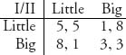
The idea is that two organisms with different sizes are competing for resources. If a Little guy meets a Big guy the Little guy is sure to eke out a barely livable subsistence but a Big guy does very well. Two Big guys who meet will barely get enough to satisfy them, while two little guys will thrive with the resources available. Our problem is to determine if being little will prevail over the generations or will Big guys eventually take over, or is it the other way around, or can they live side by side.
Begin by observing that only (3, 3) is a Nash equilibrium. Now let’s assume that a small percentage p of the population is Big, while a large majority 1 – p fraction is Little. Let’s consider the pure strategy corresponding to player I always plays Little. When two organisms meet there is probability 1 – p a Little guy meets a Big guy, and probability p a Little guy meets another Little guy. This means the expected payoff to a Little guy is
![]()
On the other hand, if player I is a Big guy, he meets another Big with probability 1 – p and a Little with probability p. The expected payoff for a Big guy is
![]()
Would player I prefer to be Big or Little? Which option gives player I a higher expected payoff, that is, when is FB(p) > FL(p)? Obviously, if 5 – 4p < 8 – 5p then all this requires is p < 3, which is always true. What we can conclude is that playing Little should not be evolutionary stable because a Big guy does better.
Is playing Big evolutionary stable? Let’s apply the same analysis. Now we assume that a small percentage of the population p is Little while a large percentage 1 – p is Big. Player I will play Big and receive expected payoff
![]()
If player I plays Little the expected payoff is
![]()
Now ask when FB(p) = 5p + 3 > FL(p) = 4p + 1 and you see that it would be true if p > –2, and that is always true. This implies that Big is indeed evolutionary stable.
As a consequence, if we have a population of Little guys and a small percentage of Big guys show up, either by mutation or invasion from somewhere else, the Big guys will have a small chance of running into another Big but will do extremely well against a Little. Bigs will thrive and cannot be overcome by the Littles. By the same token, introducing a small percentage of Littles into a population of Bigs will not materially affect the Bigs. In evolutionary terms, the Littles will not be able to invade the Bigs but Bigs can invade Littles and so Big is evolutionary stable.
Now we know how to define what it means to have evolutionary stable pure strategies.
Definition 7.1.1 Given the symmetric game (A, AT), pure strategy i* is evolutionary stable (ESS) if there is a 0 < p* < 1 so that
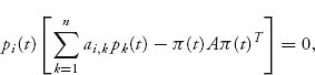
This does not have to be true for all p but for all small enough p. If we think of p as the probability a player does not use i* (but uses some other strategy j) and 1 – p as the probability a player does use i* then the expected payoff to a player using i* is
![]()
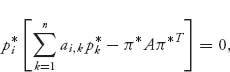
The expected payoff to a player using j against a player using i* is
![]()
The definition of ESS says that the expected payoff using i* is bigger than the expected payoff for a player using any other j, for all percentages of the players deviating from i* small enough.
Now here is an equivalent and easier to check condition. It has the advantage of not involving p. Furthermore, it will show why the fact that (3, 3) in the Little vs. Big game is a strict Nash equilibrium is not coincidental for an ESS.
Proposition 7.1.2 A pure strategy i* is an ESS if and only if
Proof Suppose that i* is an ESS. In this case (i*, i*) must be a Nash equilibrium. In fact if it wasn’t, then there is another row j so that aji* > ai*i*. By the definition of an ESS in (7.1),
![]()
Sending p → 0 in this inequality we see that the left side is strictly negative, while the right converges to zero, a contradiction. Hence, (i*, i*) must be a Nash.
Next, if (i*, i*) is a strict Nash, then it must be an ESS. To see why, since i* is strict, we must have ai*i* > aji* for any j. But then the condition (7.1) is true with p = 0 and, by continuity, will also be true for all small p > 0.
The final thing we have to answer is the case when (i*, i*) is not a strict Nash. When that happens, it means that there is a j ≠ i* which is a best response to i* so that ai*i* = aji*. But then (7.1) is the condition ai*j>ajj. That is,
![]()
for every j that is a best response to i*. ![]()
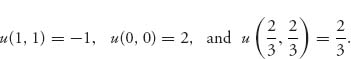
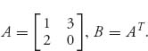
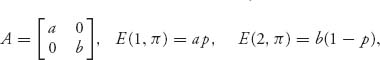
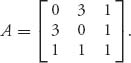
Example 7.1 1. Consider the symmetric game with
![]()
Then (i*, i*) = (1, 1) is a pure Nash equilibrium and (1) of Proposition 7.1.2 is satisfied. The best response to i* = 1 is only j = 1 which means that condition (2) is satisfied vacuously. We conclude that (1, 1) is an ESS. That is, the payoff (2, 2) as a strict Nash equilibrium is an ESS.
2. Consider the symmetric game with
![]()
There are two pure strict Nash equilibria and they are both ESSs. Again condition (2) is satisfied vacuously. (Later we will see the third Nash equilibrium is mixed and it is not an ESS.)
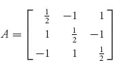
3. Consider the symmetric game with
![]()
This game also has two pure Nash equilibria neither of which is an ESS since a nonsymmetric NE cannot be an ESS. One of the Nash equilibria is at row 2, column 1, a21 = 2. If we use i* = 2, row 2 column 2 is NOT a Nash equilibrium. Condition (1) is not satisfied. The pure Nash equilibrium must be symmetric. (We will see later that the mixed Nash equilibrium is symmetric and it is an ESS.)
Now we consider the case when we have mixed ESSs. We’ll start from the beginning.
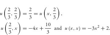
To make things simple, we assume for now that A is a 2 × 2 matrix. Then, for a strategy X = (x, 1 – x) and Y = (y, 1 − y), we will work with the expected payoffs
![]()
Because of symmetry, we have u(x, y) = v(y, x), so we really only need to talk about u(x, y) and focus on the payoff to player I.
Suppose that there is a strategy X* = (x*, 1 − x*) that is used by most members of the population and s fixed strategies X1, …, Xs, which will be used by deviants, a small proportion of the population. Again, we will refer only to the first component of each strategy, x1, x2, …, xs.
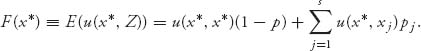
Suppose that we define a random variable Z, which will represent the strategy played by player I’s next opponent. The discrete random variable Z takes on the possible values x*, x1, x2, …, xs depending on whether the next opponent uses the usual strategy, x*, or a deviant (or mutant) strategy, x1, …, xs. We assume that the distribution of Z is given by

It is assumed that X* will be used by most opponents, so we will take 0 < p ≈ 0, to be a small, but positive number. If player I uses X* and player II uses Z, the expected payoff, also called the fitness of the strategy X*, is given by
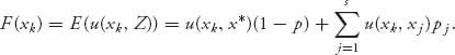
Similarly, the expected payoff to player I if she uses one of the deviant strategies xk, k = 1, 2, …, s, is
Subtracting (7.3) from (7.2), we get

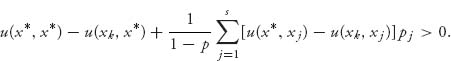
We want to know what would guarantee F(x*) > F(xk) so that x* is a strictly better, or more fit, strategy against any deviant strategy. If
![]()
then, from (7.4) we will have F(x*) > F(xk), and so no player can do better by using any deviant strategy. This defines x* as an uninvadable, or an evolutionary stable strategy. In other words, the strategy X* resists being overtaken by one of the mutant strategies X1, …, Xs, in case X* gives a higher payoff when it is used by both players than when any one player decides to use a mutant strategy, and the proportion of deviants in the population p is small enough. We need to include the requirement that p is small enough because p = ∑ j pj and we need
We can arrange this to be true if p is small but not for all 0 < p < 1.
Now, the other possibility in (7.4) is that the first term could be zero for even one xk. In that case u(x*, x*) − u(xk, x*) = 0, and the first term in (7.4) drops out for that k. In order for F(x*) > F(xk), we would now need u(x*, xj) > u(xk, xj) for all j = 1, 2, …, s. This has to hold for any xk such that u(x*, x*) = u(xk, x*). In other words, if there is even one deviant strategy that is as good as x* when played against x*, then, in order for x* to result in a higher average fitness, we must have a bigger payoff when x* is played against xj than any payoff with xk played against xj. Thus, x* played against a deviant strategy must be better than xk against any other deviant strategy xj.
We summarize these conditions as a definition.
Definition 7.1.3 A strategy X* is an ESS against (deviant strategy) strategies X1, …, Xs if either of (1) or (2) hold:
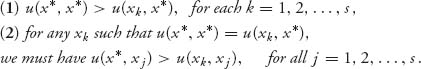
In the case when there is only one deviant strategy, s = 1, and we label X1 = X = (x, 1 − x), 0 < x < 1. That means that every player in the population must use X* or X with X as the deviant strategy. The proportion of the population using X* is 1 – p. The proportion of the population that uses the deviant strategy is p. In this case, the definition reduces to: X* is an ESS if and only if either (1) or (2) holds:
![]()
In the rest of this chapter, we consider only the case s = 1.
Remark This definition says that either X* played against X* is strictly better than any X played against x*, or, if X against X* is as good as X* against x*, then X* against any other X must be strictly better than X played against X.
Note that if X* and X are any mixed strategies and 0 < p < 1, then (1 − p) X + pX* is also a mixed strategy and can be used in an encounter between two players. Here, then, is another definition of an ESS that we will show shortly is equivalent to the first definition.
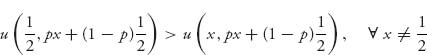
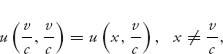
Definition 7.1.4 A strategy X* = (x*, 1 − x*) is an evolutionary stable strategy if for every strategy X = (x, 1 − x), with x ≠ x*, there is some px ![]() (0, 1), which depends on the particular choice x, such that
(0, 1), which depends on the particular choice x, such that
Remark This definition says that X* should be a good strategy if and only if this strategy played against the mixed strategy Yp ≡ p X + (1 − p)X* is better than any deviant strategy X played against Yp = p X + (1 − p)X*, given that the probability p, that a member of the population will use a deviant strategy is sufficiently small.
The left side of (7.5) is
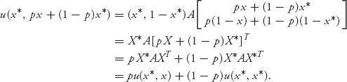
The right side of (7.5) is
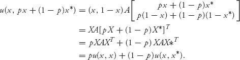
Putting them together yields that X* is an ESS according to this definition if and only if
![]()
But this condition is equivalent to
Now we can show the two definitions of ESS are equivalent.
Proposition 7.1.5 X* is an ESS according to Definition (7.3) if and only if X* is an ESS according to Definition (7.4).
Proof Suppose X* satisfies definition (7.3) from (7.2), we get
(7.7)
(7.8)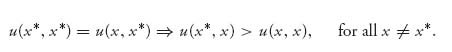
If we suppose that u(x*, x*) > u(x, x*), for all x ≠ x*, then for each x there is a small γx > 0 so that
![]()
For a fixed x ≠ x*, since γx > 0, we can find a small enough px > 0 so that for 0 < p < px we have
![]()
This says that for all 0 < p < px, we have
![]()
which means that (7.6) is true. A similar argument shows that if we assume u(x*, x*) = u(x, x*) ⇒ u(x*, x) > u(x, x) for all x ≠ x*, then (7.6) holds. So, if X* is an ESS in the sense of definition (7.3), then it is an ESS in the sense of definition (7.4).
Conversely, if X* is an ESS in the sense of definition (7.4), then for each x there is a px > 0 so that
![]()
If u(x*, x*) − u(x, x*) = 0, then since p > 0, it must be the case that u(x*, x) − u(x, x) > 0. In case u(x*, x*) − u(x′, x*) ≠ 0 for some x′ ≠ x*, sending p → 0 in
![]()
we conclude that u(x*, x*) − u(x′, x*) > 0, and this is true for every x′ ≠ x*. But that says that X* is an ESS in the sense of definition (7.3). ![]()
7.1.1 PROPERTIES OF AN ESS
1. If X*is an ESS, then (X*, X*) is a Nash equilibrium. Why? Because if it isn’t a Nash equilibrium, then there is a player who can find a strategy Y = (y, 1 − y) such that u(y, x*) > u(x*, x*). Then, for all small enough p = py, we have
![]()
This is a contradiction of the definition (7.4) of ESS. One consequence of this is that only the symmetric Nash equilibria of a game are candidates for ESSs.
2. If (X*, X*) is a strict Nash equilibrium, then X* is an ESS. Why? Because if (X*, X*) is a strict Nash equilibrium, then u(x*, x*) > u(y, x*) for any y ≠ x*. But then, for every small enough p, we would obtain
![]()
for some py > 0 and all 0 < p < py. But this defines X* as an ESS according to (7.4).
3. A symmetric Nash equilibrium X* is an ESS for a symmetric game if and only if u(x*, y) > u(y, y) for every strategy y ≠ x* that is a best response strategy to x*. Recall that Y = (y, 1 − y) is a best response to X* = (x*, 1 − x*) if
![]()
because of symmetry. In short, u(y, x*) = max0≤w≤1 u(w, x*).
4. A symmetric 2 × 2 game with A = (aij) and a11 ≠ a21, a12 ≠ a22 must have an ESS.
Let’s verify property 4.
Case 1. Suppose a11 > a21. This implies row 1, column 1 is a strict Nash equilibrium, so immediately it is an ESS. We reach the same conclusion by the same argument if a22 > a12.
Case 2. Suppose a11 < a21 and a22 < a12. In this case there is no pure Nash but there is a symmetric mixed Nash given by
![]()
Under this case 0 < x* < 1. Now direct calculation shows that
![]()
Also,
![]()
Using algebra, we get
![]()
since the denominator is negative. Thus, X* satisfies the conditions to be an ESS.
We now present a series of examples illustrating the concepts and calculations.
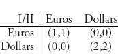
Example 7.2 In a simplified model of the evolution of currency, suppose that members of a population have currency in either euros or dollars. When they want to trade for some goods, the transaction must take place in the same currency. Here is a possible matrix representation
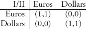
Naturally, there are three symmetric Nash equilibria X1 = (1, 0) = Y1, X2 = (0, 1) = Y2 and one mixed Nash equilibrium at ![]() These correspond to everyone using euros, everyone using dollars, or half the population using euros and the other half dollars. We want to know which, if any, of these are ESSs. We have for X1:
These correspond to everyone using euros, everyone using dollars, or half the population using euros and the other half dollars. We want to know which, if any, of these are ESSs. We have for X1:
![]()
This says X1 is ESS.
Next, for X2 we have
![]()
Again, X2 is an ESS. Note that both X1 and X2 are strict Nash equilibria and so ESSs according to properties (Section 7.1.1), part 2.
Finally for X3, we have
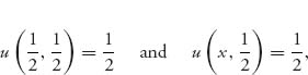
so ![]() for all
for all ![]() We now have to check the second possibility in definition (7.3):
We now have to check the second possibility in definition (7.3):
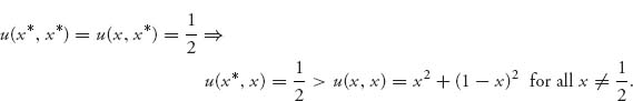
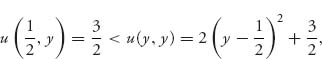
But that is false because there are plenty of x values for which this inequality does not hold. We can take, for instance ![]() to get
to get ![]() Consequently, the mixed Nash equilibrium X3 in which a player uses dollars and euros with equal likelihood is not an ESS. The conclusion is that eventually, the entire population will evolve to either all euros or all dollars, and the other currency will disappear. This seems to predict the future eventual use of one currency worldwide, just as the euro has become the currency for all of Europe.
Consequently, the mixed Nash equilibrium X3 in which a player uses dollars and euros with equal likelihood is not an ESS. The conclusion is that eventually, the entire population will evolve to either all euros or all dollars, and the other currency will disappear. This seems to predict the future eventual use of one currency worldwide, just as the euro has become the currency for all of Europe.
Example 7.3 Consider the symmetric game with

Earlier we saw that there are two pure Nash equilibria and they are both ESSs. There is also a mixed ESS given by ![]() but it is not an ESS. In fact, since
but it is not an ESS. In fact, since ![]() no matter which Y = (y, 1 − y) is used, any mixed strategy is a best response to X*. If X* is an ESS it must be true that
no matter which Y = (y, 1 − y) is used, any mixed strategy is a best response to X*. If X* is an ESS it must be true that ![]() for all
for all ![]() However,
However,
and X* is not an ESS.
Now consider the symmetric game with

We have seen that this game has two pure Nash equilibria neither of which is an ESS. There is a mixed symmetric Nash equilibrium given by ![]() and it is an ESS. In fact, we will show that
and it is an ESS. In fact, we will show that
for small enough 0 < p < 1. By calculation
and indeed for any ![]() we have
we have ![]() for any 0 < p < 1. Hence, by (7.6) X* is an ESS.
for any 0 < p < 1. Hence, by (7.6) X* is an ESS.
Example 7.4 Hawk–Dove Game. Each player can choose to act like a hawk or act like a dove, can either fight or yield, when they meet over some roadkill. The payoff matrix is
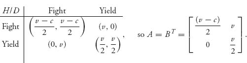
The reward for winning a fight is v > 0, and the cost of losing a fight is c > 0. Each player has an equal chance of winning a fight. The payoff to each player if they both fight is thus ![]() If hawk fights, and dove yields, hawk gets v while dove gets 0. If they both yield they both receive v/2. This is a symmetric two-person game.
If hawk fights, and dove yields, hawk gets v while dove gets 0. If they both yield they both receive v/2. This is a symmetric two-person game.
Consider the following cases:
Case 1. v > c. When the reward for winning a fight is greater than the cost of losing a fight, there is a unique symmetric Nash equilibrium at (fight, fight). In addition, it is strict, because ![]() and so it is the one and only ESS. Fighting is evolutionary stable, and you will end up with a population of fighters.
and so it is the one and only ESS. Fighting is evolutionary stable, and you will end up with a population of fighters.
Case 2. v = c. When the cost of losing a fight is the same as the reward of winning a fight, there are two nonstrict nonsymmetric Nash equilibria at (yield, fight) and (fight, yield). But there is only one symmetric, nonstrict Nash equilibrium at (fight, fight). Since u(fight, yield) = v > u(yield, yield) = v/2, the Nash equilibrium (fight, fight) satisfies the conditions in the definition of an ESS.
Case 3. c > v. Under the assumption c > v, we have two pure nonsymmetric Nash equilibria at X1 = (0, 1), Y1 = (1, 0) with payoff u(0, 1) = v/2 and X2 = (1, 0), Y2 = (0, 1), with payoff u(1, 0) = (v − c)/2. It is easy to calculate that ![]() is the symmetric mixed strategy Nash equilibrium. This is a symmetric game, and so we want to know which, if any, of the three Nash points are evolutionary stable in the sense of definition (7.3). But we can immediately eliminate the nonsymmetric equilibria.
is the symmetric mixed strategy Nash equilibrium. This is a symmetric game, and so we want to know which, if any, of the three Nash points are evolutionary stable in the sense of definition (7.3). But we can immediately eliminate the nonsymmetric equilibria.
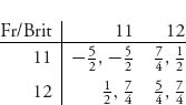
Before we consider the general case let’s take for the time being specifically v = 4, c = 6. Then ![]() so
so
Let’s consider the mixed strategy ![]() We have
We have
Since ![]() we need to show that the second case in definition (7.3) holds, namely,
we need to show that the second case in definition (7.3) holds, namely, ![]() for all
for all ![]() By algebra, this is the same as showing that
By algebra, this is the same as showing that ![]() for
for ![]() which is obvious. We conclude that
which is obvious. We conclude that ![]() is evolutionary stable.
is evolutionary stable.
For comparison purposes, let’s try to show that X1 = (0, 1) is not an ESS directly from the definition. Of course, we already know it isn’t because (X1, X1) is not a Nash equilibrium. So if we try the definition for X1 = (0, 1), we would need to have that
![]()
which is clearly false for any 0 < x ≤ 1. So X1 is not evolutionary stable.
From a biological perspective, this says that only the mixed strategy Nash equilibrium is evolutionary stable, and so always fighting, or always yielding is not evolutionary stable. Hawks and doves should fight two-thirds of the time when they meet.
In the general case with v < c, we have the mixed symmetric Nash equilibrium ![]() and since
and since
we need to check whether u(x*, x) > u(x, x). An algebra calculation shows that
![]()
Consequently, X* is an ESS.
It is not true that every symmetric game will have an ESS. The game in the next example will illustrate that.
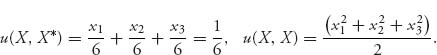
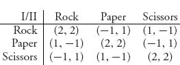
Example 7.5 We return to consideration of the rock-paper-scissors game with a variation on what happens when there is a tie. Consider the matrix
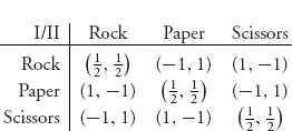
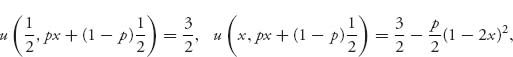
A tie in this game gives each player a payoff of ![]() so this is not a zero sum game, but it is symmetric. You can easily verify that there is one Nash equilibrium mixed strategy, and it is
so this is not a zero sum game, but it is symmetric. You can easily verify that there is one Nash equilibrium mixed strategy, and it is ![]() with expected payoff
with expected payoff ![]() to each player. (If the diagonal terms gave a payoff to each player ≥ 1, there would be many more Nash equilibria, both mixed and pure.) We claim that (X*, X*) is not an ESS.
to each player. (If the diagonal terms gave a payoff to each player ≥ 1, there would be many more Nash equilibria, both mixed and pure.) We claim that (X*, X*) is not an ESS.
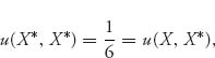
If X* is an ESS, it would have to be true that either
or
Note that this is a 3 × 3 game, and so we have to use strategies X = (x1, x2, x3) ![]() S3. Now
S3. Now ![]() where
where
and
The first possibility (7.9) does not hold.
For the second possibility condition (7.10), we have
but
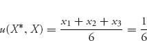
is not greater than ![]() for all mixed X ≠ X*. For example, take the pure strategy X = (1, 0, 0) to see that it fails. Therefore, neither possibility holds, and X* is not an ESS.
for all mixed X ≠ X*. For example, take the pure strategy X = (1, 0, 0) to see that it fails. Therefore, neither possibility holds, and X* is not an ESS.
Our conclusion can be phrased in this way. Suppose that one player decides to use ![]() The best response to X* is the strategy
The best response to X* is the strategy ![]() so that
so that
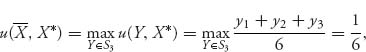
and any pure strategy, for instance ![]() will give that. But then
will give that. But then ![]() so that any deviant using any of the pure strategies can do better and will eventually invade the population. There is no uninvadable strategy.
so that any deviant using any of the pure strategies can do better and will eventually invade the population. There is no uninvadable strategy.
Remark There is much more to the theory of evolutionary stability and many extensions of the theory, as you will find in the references. In the next section, we will present one of these extensions because it shows how the stability theory of ordinary differential equations enters game theory.
Problems
7.1 In the currency game (Example 7.2), derive the same result we obtained but using the equivalent definition of ESS: X* is an evolutionary stable strategy if for every strategy X = (x, 1 − x), with x ≠ x*, there is some px ![]() (0, 1), which depends on the particular choice x, such that
(0, 1), which depends on the particular choice x, such that
![]()
Find the value of px in each case an ESS exists.
7.2 It is possible that there is an economy that uses a dominant currency in the sense that the matrix becomes
Find all Nash equilibria and determine which are ESSs.
7.3 The decision of whether or not each of two admirals should attack an island was studied in Problem 4.16. The analysis resulted in the following matrix.
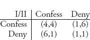
7.4 Analyze the Nash equilibria for a version of the prisoner’s dilemma game:
7.5 Determine the Nash equilibria for rock-paper-scissors with matrix
There are three pure Nash equilibria and four mixed equilibria (all symmetric). Determine which are evolutionary stable strategies, if any, and if an equilibrium is not an ESS, show how the requirements fail.
7.6 In Problem 3.18, we considered the game of the format to be used for radio stations WSUP and WHAP. The game matrix is
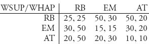
Determine which, if any of the three Nash equilibria are ESSs.
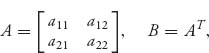
7.7 Consider a game with matrix ![]() Suppose that a b ≠ 0.
Suppose that a b ≠ 0.
7.8 Verify that X* = (x*, 1 − x*) is an ESS if and only if (X*, X*) is a Nash equilibrium and u(x*, x) > u(x, x) for every X = (x, 1 − x) ≠ X* that is a best response to X*.
7.2 Population Games
One important idea introduced by considering evolutionary stable strategies is the idea that eventually, players will choose strategies that produce a better-than-average payoff. The clues for this section are the words eventually and better-than-average. The word eventually implies a time dependence and a limit as time passes, so it is natural to try to model what is happening by introducing a time-dependent equation and let t → ∞. That is exactly what we study in this section.
Here is the setup. There are N members of a population. At random two members of the population are chosen to play a certain game against each other. It is assumed that N is a really big number, so that the probability of a faceoff between two of the same members is virtually zero.
We assume that the game they play is a symmetric two-person bimatrix game. Symmetry here again means that B = AT. Practically, it means that the players can switch roles without change. In a symmetric game it doesn’t matter who is player I and who is player II.
Assume that there are many players in the population. Any particular player is chosen from the population, chooses a mixed strategy, and plays in the bimatrix game with matrix A against any other player chosen from the population. This is called a random contest. Note that all players will be using the same payoff matrix.
The players in the population may use pure strategies 1, 2, …, n. Suppose that the percentage of players in the population using strategy j is
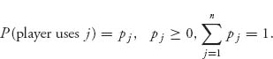
Set π = (p1, …, pn). These pi components of π are called the frequencies and represent the probability a randomly chosen individual in the population will use the strategy i. Denote by
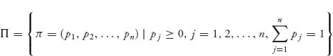
the set of all possible frequencies.
If two players are chosen from the population and player I chooses strategy i and player II chooses strategy j, we calculate the payoffs from the matrix A.
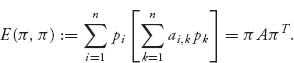
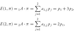
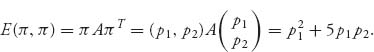
We define the fitness of a player playing strategy i = 1, 2, …, n as
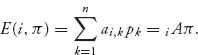
This is the expected payoff of a random contest to player I who uses strategy i against the other possible strategies 1, 2, … n, played with probabilities p1, …, pn. It measures the worth of strategy i in the population. You can see that the π looks just like a mixed strategy and we may identify E(i, π) as the expected payoff to player I if player I uses the pure strategy i and the opponent (player II) uses the mixed strategy π.
Next, we calculate the expected fitness of the entire population as
Now suppose that the frequencies π = (p1, …, pn) = π (t) ![]() Π can change with time. This is where the evolutionary characteristics are introduced. We need a model describing how the frequencies can change in time and we use the frequency dynamics as the following system of differential equations:
Π can change with time. This is where the evolutionary characteristics are introduced. We need a model describing how the frequencies can change in time and we use the frequency dynamics as the following system of differential equations:
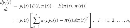
or, equivalently,
(7.12)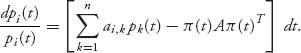
This is also called the replicator dynamics. The idea is that the growth rate at which the population percentage using strategy i changes is measured by how much greater (or less) the expected payoff (or fitness) using i is compared with the expected fitness using all strategies in the population. Better strategies should be used with increasing frequency and worse strategies with decreasing frequency. In the one-dimensional case, the right side will be positive if the fitness using pure strategy i is better than average and negative if worse than average. That makes the derivative dpi(t)/dt positive if better than average, which causes pi(t) to increase as time progresses, and strategy i will be used with increasing frequency.
We are not specifying at this point the initial conditions π(0) = (p1(0), …, pn(0)), but we know that ![]() We also note that any realistic solution of equations (7.11) must have 0 ≤ pi(t) ≤ 1 as well as
We also note that any realistic solution of equations (7.11) must have 0 ≤ pi(t) ≤ 1 as well as ![]() for all t > 0. In other words, we must have π(t)
for all t > 0. In other words, we must have π(t) ![]() Π for all t ≥ 0. Here is one way to check that: add up the equations in (7.11) to get
Π for all t ≥ 0. Here is one way to check that: add up the equations in (7.11) to get
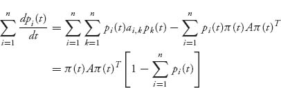
or, setting ![]()
![]()
If γ(0) = 1, the unique solution of this equation is γ(t) ≡ 1, as you can see by plugging in γ(t) = 1. Consequently, ![]() for all t ≥ 0. By uniqueness it is the one and only solution. In addition, assuming that pi(0) > 0, if it ever happens that pi(t0) = 0 for some t0 > 0, then, by considering the trajectory with that new initial condition, we see that pi(t) ≡ 0 for all t ≥ t0. This conclusion also follows from the fact that (7.11) has one and only one solution through any initial point, and zero will be a solution if the initial condition is zero. Similar reasoning, which we skip, shows that for each i, 0 ≤ pi(t) ≤ 1. Therefore π (t)
for all t ≥ 0. By uniqueness it is the one and only solution. In addition, assuming that pi(0) > 0, if it ever happens that pi(t0) = 0 for some t0 > 0, then, by considering the trajectory with that new initial condition, we see that pi(t) ≡ 0 for all t ≥ t0. This conclusion also follows from the fact that (7.11) has one and only one solution through any initial point, and zero will be a solution if the initial condition is zero. Similar reasoning, which we skip, shows that for each i, 0 ≤ pi(t) ≤ 1. Therefore π (t) ![]() Π, for all t ≥ 0, if π (0)
Π, for all t ≥ 0, if π (0) ![]() Π.
Π.
Note that when the right side of (7.11)
then dpi(t)/dt = 0 and pi(t) is not changing in time. In differential equations, a solution that doesn’t change in time will be a steady-state, equilibrium, or stationary solution. So, if there is a constant solution ![]() of
of
then if we start at π(0) = π*, we will stay there for all time and limt→∞ π(t) = π* is a steady-state solution of (7.11).
Remark If the symmetric game has a completely mixed Nash equilibrium ![]() then π* = X* is a stationary solution of (7.11). The reason is provided by the equality of payoffs Theorem 3.2.4, which guarantees that E(i, X*) = E(j, X*) = E(X*, X*) for any pure strategies i, j played with positive probability. So, if the strategy is completely mixed, then
then π* = X* is a stationary solution of (7.11). The reason is provided by the equality of payoffs Theorem 3.2.4, which guarantees that E(i, X*) = E(j, X*) = E(X*, X*) for any pure strategies i, j played with positive probability. So, if the strategy is completely mixed, then ![]() and the payoff using row i must be the average payoff to the player. But, then if E(i, X*) = E(i, π*) = E(π*, π*) = E(X*, X*), we have the right side of (7.11) is zero and then that π* = X* is a stationary solution.
and the payoff using row i must be the average payoff to the player. But, then if E(i, X*) = E(i, π*) = E(π*, π*) = E(X*, X*), we have the right side of (7.11) is zero and then that π* = X* is a stationary solution.
Example 7.6 Consider the symmetric game with
Suppose that the players in the population may use the pure strategies k ![]() {1, 2}. The frequency of using k is pk(t) at time t ≥ 0, and it is the case that π(t) = (p1(t), p2(t))
{1, 2}. The frequency of using k is pk(t) at time t ≥ 0, and it is the case that π(t) = (p1(t), p2(t)) ![]() Π . Then the fitness of a player using k = 1, 2 becomes
Π . Then the fitness of a player using k = 1, 2 becomes
and the average fitness in the population is
We end up with the following system of equations:
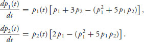
We are interested in the long-term behavior limt→∞ pi(t) of these equations because the limit is the eventual evolution of the strategies. The steady-state solution of these equations occurs when dpi(t)/dt = 0, which, in this case implies that
![]()
Since both p1 and p2 cannot be zero (because p1 + p2 = 1), you can check that we have steady-state solutions:

The arrows in Figure 7.1 show the direction a trajectory (=solution of the frequency dynamics) will take as time progresses depending on the starting condition. You can see in the figure that no matter where the initial condition is inside the square (p1, p2) ![]() (0, 1) × (0, 1), the trajectories will be sucked into the solution at the point
(0, 1) × (0, 1), the trajectories will be sucked into the solution at the point ![]() as the equilibrium solution.
as the equilibrium solution.
If, however, we start exactly at the edges p1(0) = 0, p2(0) = 1 or p1(0) = 1, p2(0) = 0, then we stay on the edge forever. Any deviation off the edge gets the trajectory sucked into ![]() where it stays forever.
where it stays forever.
Remark Whenever there are only two pure strategies used in the population, we can simplify down to one equation for p(t) using the substitutions p1(t) = p(t), p2(t) = 1 − p(t). Since
![]()
Equation (7.11) then becomes
(7.13)![]()
and we must have 0 ≤ p(t) ≤ 1. The equation for p2 in (7.11) is redundant.
FIGURE 7.1 Stationary solution at ![]()
For Example 7.6, the equation reduces to
![]()
which is no easier to solve exactly. This equation can be solved implicitly using integration by parts to give the implicitly defined solution
![]()
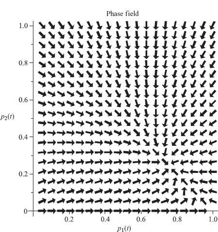
This is valid only away from the stationary points ![]() because, as you can see, the logarithm is a problem at those points. Figure 7.2 shows the direction field of p(t) versus time on the left and the direction field superimposed with the graphs of four trajectories starting from four different initial conditions, two on the edges, and two in the interior of (0, 1). The interior trajectories get pulled quickly as t → ∞ to the steady-state solution
because, as you can see, the logarithm is a problem at those points. Figure 7.2 shows the direction field of p(t) versus time on the left and the direction field superimposed with the graphs of four trajectories starting from four different initial conditions, two on the edges, and two in the interior of (0, 1). The interior trajectories get pulled quickly as t → ∞ to the steady-state solution ![]() while the trajectories that start on the edges stay there forever.
while the trajectories that start on the edges stay there forever.
FIGURE 7.2 Direction field and trajectories for dp(t)/dt = p(t)(1 − p(t))(− 4p(t) + 3), p(t) versus time with four initial conditions.
In the long run, as long as the population is not using strategies on the edges (i.e., pure strategies), the population will eventually use the pure strategy k = 1 exactly 75% of the time and strategy k = 2 exactly 25% of the time.
Now, the idea is that the limit behavior of π(t) will result in conclusions about how the population will evolve regarding the use of strategies. But that is what we studied in the previous section on evolutionary stable strategies. There must be a connection.
Example 7.7 In an earlier Problem 7.7, we looked at the game with matrix ![]() and assumed a b ≠ 0. You showed the following:
and assumed a b ≠ 0. You showed the following:
The system of equations for this population game becomes
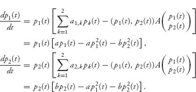
We can simplify using the fact that p2 = 1 − p1 to get
Now we can see that if a > 0 and b < 0, the right side is always > 0, and so p1(t) increases while p2(t) decreases. Similarly, if a < 0, b > 0, the right side of (7.14) is always < 0 and so p1(t) decreases while p2(t) increases. In either case, as t → ∞ we converge to either (p1, p2) = (1, 0) or (0, 1), which is at the unique ESS for the game. When p1(t) must always increase, for example, but cannot get above 1, we know it must converge to 1.
In the case when a > 0, b > 0 there is only one mixed Nash (which is not an ESS) occurring with the mixture ![]() It is not hard to see that in this case, the trajectory (p1(t), p2(t)) will converge to one of the two pure Nash equilibria that are the ESSs of this game. In fact, if we integrate the differential equation, which is (7.14), replacing p2 = 1 − p1 and p = p1, we have using integration by partial fractions
It is not hard to see that in this case, the trajectory (p1(t), p2(t)) will converge to one of the two pure Nash equilibria that are the ESSs of this game. In fact, if we integrate the differential equation, which is (7.14), replacing p2 = 1 − p1 and p = p1, we have using integration by partial fractions
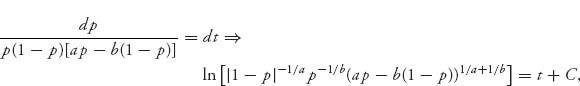
or
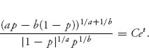
As t → ∞, assuming C > 0, the right side goes to ∞. There is no way that could happen on the left side unless p → 0 or p → 1. It would be impossible for the left side to become infinite if limt→∞ p(t) is strictly between 0 and 1.
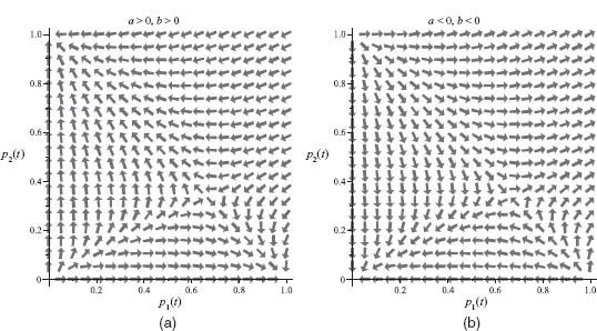
We illustrate the case a > 0, b > 0 in Figure 7.3a for choices a = 1, b = 2, and several distinct initial conditions. You can see that limt→∞ p2(t) = 0 or = 1, so it is converging to a pure ESS as long as we do not start at ![]()
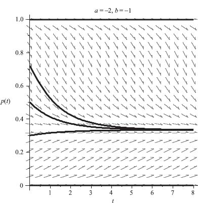
In the case a < 0, b < 0 the trajectories converges to the mixed Nash equilibrium, which is the unique ESS. This is illustrated in Figure 7.3b with a = −1, b = −2, and you can see that ![]() and so
and so ![]() The phase portraits in Figure 7.4 show clearly what is happening if you follow the arrows.
The phase portraits in Figure 7.4 show clearly what is happening if you follow the arrows.
The graphs in Figures 7.3 and 7.4 were created using the following Maple commands:
>restart:a:=1:b:=2:
> ode:=diff(p1(t), t)=p1(t)*(a*p1(t)-a*p1(t)^2-b*p2(t)^2),
       diff(p2(t), t)=p2(t)*(b*p2(t)-a*p1(t)^2-b*p2(t)^2);
> with(DEtools):
> DEplot([ode], [p1(t), p2(t)], t=0..20,
       [[p1(0)=.8, p2(0)=.2],
             [p1(0)=.1, p2(0)=.9], [p1(0)=2/3, p2(0)=1/3]],
       stepsize=.05, p1=0..1, p2=0..1,
       scene=[p1(t), p2(t)], arrows=large, linecolor=black,
       title="a>0, b>0");
> DEplot([ode], [p1(t), p2(t)], t=0..20,
       [[p1(0)=.8, p2(0)=.2], [p1(0)=.4, p2(0)=.6],
       [p1(0)=.6, p2(0)=.4], [p1(0)=.75, p2(0)=.25],
       [p1(0)=.1, p2(0)=.9], [p1(0)=2/3, p2(0)=1/3]],
       stepsize=.01, p1=0..1, p2=0..1,
       scene=[t, p2(t)], arrows=large, linecolor=black,
       title="a>0, b>0");
FIGURE 7.3 (a) a > 0, b > 0;. (b) a < 0, b < 0.
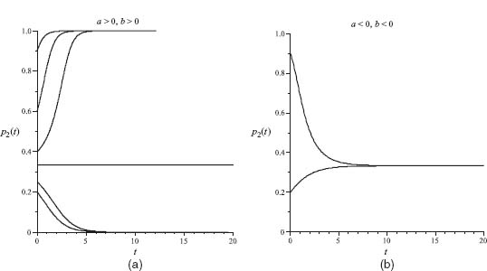
FIGURE 7.4 (a) Convergence to ESS (1, 0) or (0, 1). (b) Convergence to the mixed ESS.
Remark Example 7.7 is not as special as it looks because if we are given any two-player symmetric game with matrix
then the game is equivalent to the symmetric game with matrix
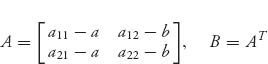
for any a, b, in the sense that they have the same set of Nash equilibria. This was Problem 3.28. In particular, if we take a = a21 and b = a12, we have the equivalent matrix game
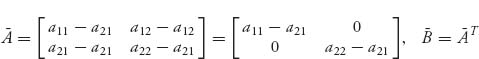
and so we are in the case discussed in the example.
Let’s step aside and write down some results we need from ordinary differential equations. Here is a theorem guaranteeing existence and uniqueness of solutions of differential equations.
Theorem 7.2.1 Suppose that you have a system of differential equations
Assume that ![]() and ∂f/∂pi are continuous. Then for any initial condition π(0) = π0, there is a unique solution up to some time T > 0.
and ∂f/∂pi are continuous. Then for any initial condition π(0) = π0, there is a unique solution up to some time T > 0.
Definition 7.2.2 A steady-state (or stationary, or equilibrium, or fixed-point) solution of the system of ordinary differential equations (7.15) is a constant vector π* that satisfies f(π*) = 0. It is (locally) stable if for any ε > 0 there is a δ > 0 so that every solution of the system with initial condition π0 satisfies
![]()
A stationary solution of (7.15) is (locally) asymptotically stable if it is locally stable and if there is ρ > 0 so that
The set
![]()
is called the basin of attraction of the steady state π*. Here π(t) is a trajectory through the initial point π(0) = π0. If every initial point that is possible is in the basin of attraction of π*, we say that the point π* is globally asymptotically stable.
Stability means that if you have a solution of the equations (7.15) that starts near the stationary solution, then it will stay near the stationary solution as time progresses. Asymptotic stability means that if a trajectory starts near enough to π*, then it must eventually converge to π*. For a system of two equations, such as those that arise with 2 × 2 games, or to which a 3 × 3 game may be reduced, we have the criterion given in the following theorem.
Theorem 7.2.3 A steady-state solution ![]() of the system
of the system
is asymptotically stable if
![]()
and
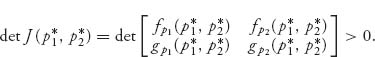
If either fp1 + g p2 > 0 or ![]() the steady-state solution
the steady-state solution ![]() is unstable (i.e., not stable).
is unstable (i.e., not stable).
The J matrix in the proposition is known as the Jacobian matrix of the system.
Example 7.8 If there is only one equation p′ = f(p), (where ′ = d/dt) then a steady state p* is asymptotically stable if f′(p*) < 0 and unstable if f′(p*) > 0. It is easy to see why that is true in the one-dimensional case. Set x(t) = p(t) − p*, so now we are looking at limt→∞ x(t) and testing whether that limit is zero. By Taylor’s theorem
![]()
should be true up to first-order terms. The solution of this linear equation is x(t) = C exp[f′(p*)t]. If f′(p*) < 0, we see that limt→∞ x(t) = 0, and if f′(p*) > 0, then limt→∞ x(t) does not exist. So that is why stability requires f′(p*) < 0.
Consider the differential equation
![]()
The stationary states are ![]() but only two of these are asymptotically stable. These are the pure states x = 0, 1, while the state
but only two of these are asymptotically stable. These are the pure states x = 0, 1, while the state ![]() is unstable because no matter how small you perturb the initial condition, the solution will eventually be drawn to one of the other asymptotically stable solutions. As t → ∞, the trajectory moves away from
is unstable because no matter how small you perturb the initial condition, the solution will eventually be drawn to one of the other asymptotically stable solutions. As t → ∞, the trajectory moves away from ![]() unless you start at exactly that point. Figure 7.5 shows this and shows how the arrows lead away from
unless you start at exactly that point. Figure 7.5 shows this and shows how the arrows lead away from ![]()
Checking the stability condition for ![]() we have
we have
f′(x) = −1 + 6x − 6x2, and f′(0) = f′(1) = −1 < 0, while ![]() and so x = 0, 1 are asymptotically stable, while
and so x = 0, 1 are asymptotically stable, while ![]() is not.
is not.
FIGURE 7.5 Trajectories of dx/dt = −x(1 − x)(1 − 2x); ![]() is unstable.
is unstable.
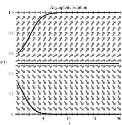
FIGURE 7.6 Convergence to p* = 1.
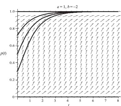
FIGURE 7.7 Mixed Nash not stable.
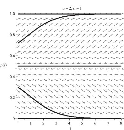
FIGURE 7.8 Convergence to the mixed ESS X* = (b/(a + b), a/(a + b)), in case a < 0, b < 0.
Now here is the connection for evolutionary game theory.
Theorem 7.2.4 In any 2 × 2 game, a strategy ![]() is an ESS if and only if the system (7.11) has
is an ESS if and only if the system (7.11) has ![]() as an asymptotically stable-steady state.
as an asymptotically stable-steady state.
Before we indicate the proof of this, let’s recall the definition of what it means to be an ESS. X* is an ESS if and only if either E(X*, X*) > E(Y, X*), for all strategies Y ≠ X* or E(X*, X*) = E(Y, X*) ⇒ E(X*, Y) > E(Y, Y), ![]() Y ≠ X*.
Y ≠ X*.
Proof Now we will show that any ESS of a 2 × 2 game must be asymptotically stable. We will use the stability criterion in Theorem 7.2.3 to do that. Because there are only two pure strategies, we have the equation for π = (p, 1 − p):
![]()
Because of an earlier Problem 7.7, we will consider only the case where
and, in general, a = a11 − a21, b = a22 − a12. Then
![]()
and
![]()
The three steady-state solutions where f(p) = 0 are p* = 0, 1, ![]() Now consider the following cases:
Now consider the following cases:
Case 1. a b < 0. In this case, there is a unique strict symmetric Nash equilibrium and so the ESSs are either X = (1, 0) (when a > 0, b < 0), or X = (0, 1) (when a < 0, b > 0). We look at a > 0, b < 0 and the steady-state solution p* = 1. Then, f′(1) = 2a + 4b − 3a − 3b − b = − a < 0, so that p* = 1 is asymptotically stable. Similarly, if a < 0, b > 0, the ESS is X = (0, 1) and p* = 0 is asymptotically stable. For an example, if we take a = 1, b = −2, Figure 7.6 shows convergence to p* = 1 for trajectories from fours different initial conditions.
Case 2. a > 0, b > 0. In this case, there are three symmetric Nash equilibria: X1 = (1, 0), X2 = (0, 1), and the mixed Nash X3 = (γ, 1 − γ), γ = b/(a + b). The two pure Nash X1, X2 are strict and thus are ESSs by the properties 7.9. The mixed Nash is not an ESS because E(X3, X3) = a γ is not larger than E(Y, X3) = a γ, ![]() Y ≠ X3 (they are equal), and taking Y = (1, 0), E(Y, Y) = E(1, 1) = a > aγ = E(X3, 1). Consequently, X3 does not satisfy the criteria to be an ESS. Hence, we only need consider the stationary solutions p* = 0, 1. But then, in the case a > 0, b > 0, we have f′(0) = −b < 0 and f′(1) = −a < 0, so they are both asymptotically stable. This is illustrated in the Figure 7.7 with a = 2, b = 1.
Y ≠ X3 (they are equal), and taking Y = (1, 0), E(Y, Y) = E(1, 1) = a > aγ = E(X3, 1). Consequently, X3 does not satisfy the criteria to be an ESS. Hence, we only need consider the stationary solutions p* = 0, 1. But then, in the case a > 0, b > 0, we have f′(0) = −b < 0 and f′(1) = −a < 0, so they are both asymptotically stable. This is illustrated in the Figure 7.7 with a = 2, b = 1.
You can see that from any initial condition ![]() the trajectory will converge to the stationary solution p* = 0. For any initial condition
the trajectory will converge to the stationary solution p* = 0. For any initial condition ![]() the trajectory will converge to the stationary solution p* = 1, and only for
the trajectory will converge to the stationary solution p* = 1, and only for ![]() will the trajectory stay at
will the trajectory stay at ![]() is unstable.
is unstable.
Case 3. a < 0, b < 0. In this case, there are two strict but asymmetric Nash equilibria and one symmetric Nash equilibrium X = (γ, 1 − γ). This symmetric X is an ESS because
and for every Y ≠ X,
![]()
since a < 0, b < 0. Consequently the only ESS is X = (γ, 1 − γ), and so we consider the steady state p* = γ. Then
and so p* = γ is asymptotically stable. For an example, if we take a = −2, b = −1, we get Figure 7.8, in which all interior initial conditions lead to convergence to ![]()
Figure 7.8 was created with the Maple commands:
> with(plots): with(DEtools):
> DEplot(D(x)(t)=(x(t)*(1-x(t))*(-2*x(t)+1*(1-x(t)))),
          x(t), t=0..8,
          [[x(0)=0], [x(0)=1], [x(0)=.5], [x(0)=.3], [x(0)=0.72]],
          title='a=-2, b=-1', colour=magenta, linecolor=
          [gold, yellow,
          black, red, blue], stepsize=0.05, labels=['t', 'p(t)']);
It is important to remember that if the trajectory starts exactly at one of the stationary solutions, then it stays there forever. It is starting nearby and seeing where it goes that determines stability.
We have proved that any ESS of a 2 × 2 game must be asymptotically stable. We skip the opposite direction of the proof and end this section by reviewing the remaining connections between Nash equilibria, ESSs, and stability. The first is a summary of the connections with Nash equilibria:
The converse statements do not necessarily hold. The verification of all these statements, and much more, can be found in the book by Weibull (1995). Now here is the main result for ESSs and stability.
Theorem 7.2.5 If X* is an ESS, then X* is an asymptotically stable stationary solution of (7.11). In addition, if X* is completely mixed, then it is globally asymptotically stable.
Again, the converse does not necessarily hold.
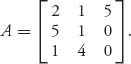
Example 7.9 In this example, we consider a 3 × 3 symmetric game so that the frequency dynamics is a system in the three variables (p1, p2, p3). Let’s look at the game with matrix
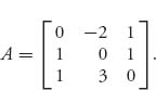
This game has Nash equilibria
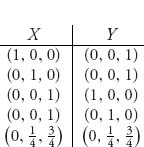
There is only one symmetric Nash equilibrium ![]() It will be an ESS because we will show that u(Y, Y) < u(X*, Y) for every best response strategy Y ≠ X* to the strategy X*. By properties 7.9(3), we then know that X* is an ESS.
It will be an ESS because we will show that u(Y, Y) < u(X*, Y) for every best response strategy Y ≠ X* to the strategy X*. By properties 7.9(3), we then know that X* is an ESS.
First, we find the set of best response strategies Y. To do that, calculate
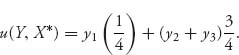
It is clear that u is maximized for y1 = 0, y2 + y3 = 1. This means that any best response strategy must be of the form Y = (0, y, 1 − y), where 0 ≤ y ≤ 1.
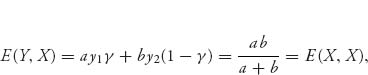
Next, taking any best response strategy, we have
![]()
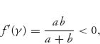
We have to determine whether ![]() for all
for all ![]() This is easy to do by calculus since
This is easy to do by calculus since ![]() has a minimum at
has a minimum at ![]() and
and ![]() Here are the Maple commands to get all of this:
Here are the Maple commands to get all of this:
> restart:with(LinearAlgebra):
> A:=Matrix([[0, -2, 1], [1, 0, 1], [1, 3, 0]]);
> X:=<0, 1/4, 3/4>; Y:=<y1, y2, y3>;
> uYY:=expand(Transpose(Y).A.Y); uYX:=expand(Transpose(Y).A.X);
> with(Optimization):
> Maximize(uYX, {y1+y2+y3=1, y1>=0, y2>=0, y3>=0});
> uXY:=Transpose(X).A.Y;
> w:=subs(y1=0, y2=y, y3=1-y, uYY); v:=subs(y1=0, y2=y, y3=1-y, uXY);
> plot(w-v, y=0..1);
The last plot, exhibited in Figure 7.9, shows that u(Y, Y) < u(X*, Y) for best response strategies, Y.
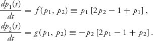
The replicator dynamics (7.11) for this game are as follows:
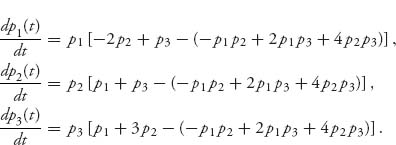
Since p1 + p2 + p3 = 1, they can be reduced to two equations to which we may apply the stability theorem. The equations become
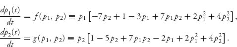
The steady-state solutions are given by the solutions of the pair of equations f(p1, p2) = 0, g(p1, p2) = 0, which make the derivatives zero and are given by
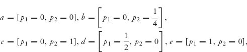
and we need to analyze each of these. We start with the condition from Theorem 7.2.3 that fp1 + gp2 < 0. Calculation yields
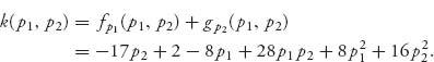
Directly plugging our points into k(p1, p2), we see that
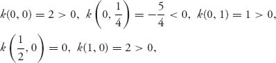
and since we only need to consider the negative terms as possibly stable, we are left with the one possible asymptotically stable value ![]()
Next, we check the Jacobian at that point and get
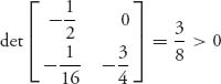
By the stability Theorem 7.2.3 ![]() is indeed an asymptotically stable solution, and hence a Nash equilibrium and an ESS. Figure 7.10 shows three trajectories (p1(t), p2(t)) starting at time t = 0 from the initial conditions (p1(0), p2(0)) = (0.1, 0.2), (0.6, 0.2), (0.33, 0.33).
is indeed an asymptotically stable solution, and hence a Nash equilibrium and an ESS. Figure 7.10 shows three trajectories (p1(t), p2(t)) starting at time t = 0 from the initial conditions (p1(0), p2(0)) = (0.1, 0.2), (0.6, 0.2), (0.33, 0.33).
We see the asymptotic convergence of (p1(t), p2(t)) to ![]() Since p1 + p2 + p3 = 1, this means
Since p1 + p2 + p3 = 1, this means ![]() It also shows a trajectory starting from p1 = 0, p2 = 0 and shows that the trajectory stays there for all time.
It also shows a trajectory starting from p1 = 0, p2 = 0 and shows that the trajectory stays there for all time.
Figure 7.10 was obtained using the following Maple commands:
> restart:with(DEtools):with(plots):with(LinearAlgebra):
> A:=Matrix([[0, -2, 1], [1, 0, 1], [1, 3, 0]]);
> X:=<x1, x2, x3>;
> Transpose(X).A.X;
> s:=expand(%);
> L:=A.X;
> L[1]-s;L[2]-s;L[3]-s;
> DEplot3d({D(p1)(t)=p1(t)*(-2*p2(t)+p3(t)+p1(t)*p2(t)
                        -2*p1(t)*p3(t)-4*p2(t)*p3(t)),
            D(p2)(t)=p2(t)*(p1(t)+p3(t)+p1(t)*p2(t)
                        -2*p1(t)*p3(t)-4*p2(t)*p3(t)),
            D(p3)(t)=p3(t)*(p1(t)+3*p2(t)+p1(t)*p2(t)
                        -2*p1(t)*p3(t)-4*p2(t)*p3(t))},
            {p1(t), p2(t), p3(t)},
            t=0..10, [[p1(0)=0.1, p2(0)=0.2, p3(0)=.7],
                      [p1(0)=0.6, p2(0)=.2, p3(0)=.2],
                      [p1(0)=1/3, p2(0)=1/3, p3(0)=1/3],
                      [p1(0)=0, p2(0)=0, p3(0)=1]],
            scene=[t, p1(t), p2(t)],
            stepsize=.1, linecolor=t);
The right sides of the frequency equations are calculated in L[i] − s, i = 1, 2, 3 and then explicitly entered in the DEplot3d command. Note the command scene = [t, p1(t), p2(t)] gives the plot viewing p1(t), p2(t) versus time. If you want to see p1 and p3 instead, then this is the command to change. These commands result in Figure 7.10.
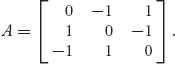
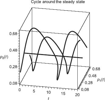
Example 7.10 This example also illustrates instability with cycling around the Nash mixed strategy as shown in Figure 7.11. The game matrix is
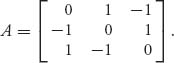
The system of frequency equations, after making the substitution p3 = 1 − p1 − p2, becomes
The steady-state solutions are (0, 0), (0, 1), (1, 0), and ![]() Then
Then
![]()
and, evaluating at the stationary points,
![]()
The steady-state solution (0, 0) is indeed asymptotically stable since the determinant of the Jacobian at that point is readily calculated to be J = 1 > 0, and so Theorem 7.2.3 tells us that (p1, p2, p3) = (0, 0, 1) is asymptotically stable. On the other hand, the unique mixed strategy corresponding to ![]() completely violates the conditions of the theorem because
completely violates the conditions of the theorem because ![]() as well as
as well as ![]()
It is unstable, as is shown in Figure 7.11.
Three trajectories are shown starting from the points (0.1, 0.2), (0.6, 0.2), and (0.33, 0.33). You can see that unless the starting position is exactly at (0.33, 0.33), the trajectories will cycle around and not converge to the mixed strategy.
Finally, a somewhat automated set of Maple commands to help with the algebra are given:
> restart:with(DEtools):with(plots):with(LinearAlgebra):
> A:=Matrix([[0, 1, -1], [-1, 0, 1], [1, -1, 0]]);
> X:=<x1, x2, x3>;
> Transpose(X).A.X;
> s:=expand(%);
> L:=A.X; L[1]-s;L[2]-s;L[3]-s;
> ode:={D(p1)(t)=p1(t)*(p2(t)-p3(t)),
           D(p2)(t)=p2(t)*(-p1(t)+p3(t)),
           D(p3)(t)=p3(t)*(p1(t)-p2(t))};
> subs(p3(t)=1-p1(t)-p2(t), ode);
> G:=simplify(%);
> DEplot3d({G[1], G[2]}, {p1(t), p2(t)}, t=0..20,
               [[p1(0)=0.1, p2(0)=0.2],
               [p1(0)=0.6, p2(0)=.2],
               [p1(0)=1/3, p2(0)=1/3]],
               scene=[t, p1(t), p2(t)],
               stepsize=.1, linecolor=t,
               title="Cycle around the steady state");
Remember that Maple makes X:=<x1, x2, x3> a column vector, and that is why we need Transpose(X).A.X to calculate E(X, X).
Problems
7.9 Consider a game in which a seller can be either honest or dishonest and a buyer can either inspect or trust (the seller). One game model of this is the matrix ![]() where the rows are inspect and trust, and the columns correspond to dishonest and honest.
where the rows are inspect and trust, and the columns correspond to dishonest and honest.
7.10 Analyze all stationary solutions for the game with matrix ![]()
7.11 Consider the symmetric game with matrix
7.12 Consider the symmetric game with matrix
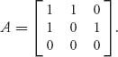
Show that X = (1, 0, 0) is an ESS that is asymptotically stable for (7.11).
7.13 The simplest version of the rock-paper-scissors game has matrix
7.14 Find the frequency dynamics (7.11) for the game
7.15 Consider the symmetric game with matrix 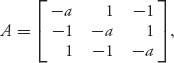 where a > 0. Show that
 ![]() is an ESS for any a > 0. Compare with Problem 7.13b.
is an ESS for any a > 0. Compare with Problem 7.13b.
7.16 Consider the symmetric game with matrix 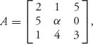 where α is a real number. This problem shows that a stable equilibrium of the replicator dynamics need not be an ESS.
Remark Do populations always choose a better strategy in the long run? There is a fictional story that implies that may not always be the case. The story starts with a measurement. In the United States, the distance between railroad rails is 4 feet 8.5 inches. Isn’t that strange? Why isn’t it 5 feet, or 4 feet? The distance between rails determines how rail cars are built, so wouldn’t it be easier to build a car with exact measurements, that determine all the parts in the drive train?
Why is that the measurement chosen?
Well, that’s the way they built them in Great Britain, and it was immigrants from Britain who built the US railroads.
Why did the English choose that measurement for the railroads in England?
Because, before there were railroads there were tramways, and that’s the measurement they chose for the tramways. (A tramway is a light-rail system for passenger trams.)
Why?
Because they used the same measurements as the people who built wagons for the wheel spacing.
And why did the wagon builders use that measurement?
Because the spacing of the wheel ruts in the old roads had that spacing, and if they used another spacing, the wagon wheels would break apart.
How did the road ruts get that spacing?
The Romans’ chariots for the legions made the ruts, and since Rome conquered most of the known world, the ruts ended up being the same almost everywhere they traveled because they were made by the same version of General Motors then, known as Imperial Chariots, Inc.
And why did they choose the spacing that started this story?
Well, that is exactly the width the chariots need to allow two horse’s rear ends to fit. And that is how the world’s most advanced transportation system is based on 4 feet 8.5 inches.
Bibliographic Notes
Evolutionary games can be approached with two distinct goals in mind. The first is the matter of determining a way to choose a correct Nash equilibrium in games with multiple equilibria. The second is to model biological processes in order to determine the eventual evolution of a population. This was the approach of Maynard-Smith and Price (see Vincent and Brown’s book (2005) for references and biologic applications) and has led to a significant impact in biology, both experimental and theoretical. Our motivation for the definition of evolutionary stable strategy is the very nice derivation in the treatise by Mesterton-Gibbons (2000). The equivalent definitions, some of which are easier to apply, are standard and appear in the literature (e.g., Weibull 1995; Vincent and Brown, 2005) as are many more results. The hawk–dove game is a classic example appearing in all books dealing with this topic. The rock-paper-scissors game is an illustrative example of a wide class of games (see the book by Weibull (1995) for a lengthy discussion of rock-paper-scissors).
Population games are a natural extension of the idea of evolutionary stability by allowing the strategies to change with time and letting time become infinite. The stability theory of ordinary differential equations can now be brought to bear on the problem (see the book by Scheinermann (1996) for the basic theory of stability). The first derivation of the replicator equations seems to have been due to Taylor and Jonker in the article in Jonker and Taylor (1978). Hofbauer and Sigmund, who have made important contributions to evolutionary game theory, have published recently an advanced survey of evolutionary dynamics in Hofbauer and Sigmund (2003). Refer to the book by Gintis (2000) for an exercise-based approach to population games and extensions.
FIGURE 7.9 Plot of ![]()
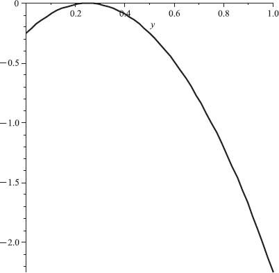
FIGURE 7.10 Convergence to ![]() from three different initial conditions.
from three different initial conditions.
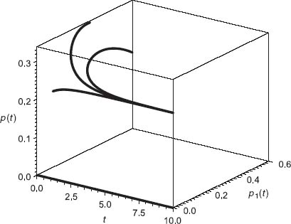
FIGURE 7.11 ![]() is unstable.
is unstable.
1 John Maynard-Smith, F.R.S. (January 6, 1920−April 19, 2004) was a British biologist and geneticist. George R. Price (1922–January 6, 1975) was an American population geneticist. He and Maynard-Smith introduced the concept of the evolutionary stable strategy (ESS).