This chapter covers

• Considering options for the various steps in the genetic algorithm life cycle

• Adjusting a genetic algorithm to solve varying problems

• The advanced parameters for configuring a genetic algorithm life cycle based on different scenarios, problems, and datasets

NOTE Chapter 4 is a prerequisite to this chapter.

Evolutionary algorithm life cycle

The general life cycle of a genetic algorithm is outlined in chapter 4. In this chapter, we consider other problems that may be suitable to be solved with a genetic algorithm, why some of the approaches demonstrated thus far won’t work, and alternative approaches.

As a reminder, the general life cycle of a genetic algorithm is as follows:

• Creating a population—Creating a random population of potential solutions.

• Measuring fitness of individuals in the population—Determining how good a specific solution is. This task is accomplished by using a fitness function that scores solutions to determine how good they are.

• Selecting parents based on their fitness—Selecting pairs of parents that will reproduce offspring.

• Reproducing individuals from parents—Creating offspring from their parents by mixing genetic information and applying slight mutations to the offspring.

• Populating the next generation—Selecting individuals and offspring from the population that will survive to the next generation.

Keep the life cycle flow (depicted in figure 5.1) in mind as we work through this chapter.

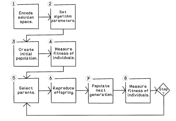
Figure 5.1 Genetic algorithm life cycle

This chapter starts by exploring alternative selection strategies; these individual approaches can be generically swapped in and out for any genetic algorithm. Then it follows three scenarios that are tweaks of the Knapsack Problem (chapter 4) to highlight the utility of the alternative encoding, crossover, and mutation approaches (figure 5.2).

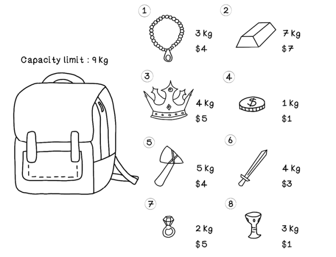
Figure 5.2 The example Knapsack Problem

Alternative selection strategies

In chapter 4, we explored one selection strategy: roulette-wheel selection, which is one of the simplest methods for selecting individuals. The following three selection strategies help mitigate the problems of roulette-wheel selection; each has advantages and disadvantages that affect the diversity of the population, which ultimately affects whether an optimal solution is found.

Rank selection: Even the playing field

One problem with roulette-wheel selection is the vast differences in the magnitude of fitness between chromosomes. This heavily biases the selection toward choosing individuals with high fitness scores or giving poor-performing individuals a larger chance of selection than desired. This problem affects the diversity of the population. More diversity means more exploration of the search space, but it can also make finding optimal solutions take too many generations.

Rank selection aims to solve this problem by ranking individuals based on their fitness and then using each individual’s rank as the value for calculating the size of its slice on the wheel. In the Knapsack Problem, this value is a number between 1 and 16, because we’re choosing among 16 individuals. Although strong individuals are more likely to be selected and weaker ones are less likely to be selected even though they are average, each individual has a fairer chance of being selected based on rank rather than exact fitness. When 16 individuals are ranked, the wheel looks slightly different from roulette-wheel selection (figure 5.3).

Figure 5.3 Example of rank selection

Figure 5.4 compares roulette-wheel selection and rank selection. It is clear that rank selection gives better-performing solutions a better chance of selection.

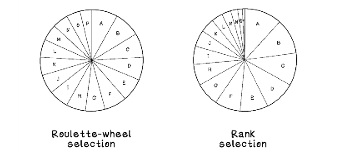
Figure 5.4 Roulette-wheel selection vs. rank selection

Tournament selection: Let them fight

Tournament selection plays chromosomes against one other. Tournament selection randomly chooses a set number of individuals from the population and places them in a group. This process is performed for a predetermined number of groups. The individual with the highest fitness score in each respective group is selected. The larger the group, the less diverse it is, because only one individual from each group is selected. As with rank selection, the actual fitness score of each individual is not the key factor in selecting individuals globally.

When 16 individuals are allocated to four groups, selecting only 1 individual from each group results in the choice of 4 of the strongest individuals from those groups. Then the 4 winning individuals can be paired to reproduce (figure 5.5).

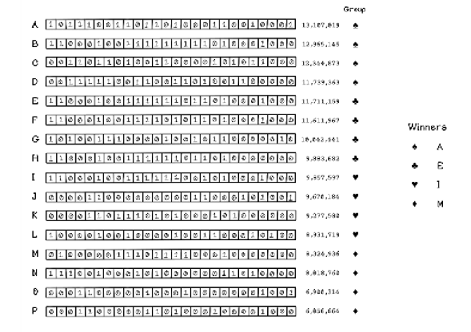
Figure 5.5 Example of tournament selection

Elitism selection: Choose only the best

The elitism approach selects the best individuals in the population. Elitism is useful for retaining strong-performing individuals and eliminating the risk that they will be lost through other selection methods. The disadvantage of elitism is that the population can fall into a local best solution space and never be diverse enough to find global bests.

Elitism is often used in conjunction with roulette-wheel selection, rank selection, and tournament selection. The idea is that several elite individuals are selected to reproduce, and the rest of the population is filled with individuals by means of one of the other selection strategies (figure 5.6).

Figure 5.6 Example of elitism selection

Chapter 4 explores a problem in which including items in or excluding items from the knapsack was important. A variety of problem spaces require a different encoding because binary encoding won’t make sense. The following three sections describe these scenarios.

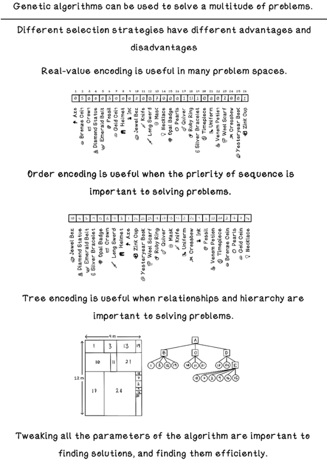
Real-value encoding: Working with real numbers

Consider that the Knapsack Problem has changed slightly. The problem remains choosing the most valuable items to fill the weight capacity of the knapsack. But the choice involves more than one unit of each item. As shown in table 5.1, the weights and values remain the same as the original dataset, but a quantity of each item is included. With this slight adjustment, a plethora of new solutions are possible, and one or more of those solutions may be more optimal, because a specific item can be selected more than once. Binary encoding is a poor choice in this scenario. Real-value encoding is better suited to representing the state of potential solutions.

Table 5.1 Knapsack capacity: 6,404,180 kg

Item ID	Item name	Weight (kg)	Value ($)	Quantity
1	Axe	32,252	68,674	19
2	Bronze coin	225,790	471,010	14
3	Crown	468,164	944,620	2
4	Diamond statue	489,494	962,094	9
5	Emerald belt	35,384	78,344	11
6	Fossil	265,590	579,152	6
7	Gold coin	497,911	902,698	4
8	Helmet	800,493	1,686,515	10
9	Ink	823,576	1,688,691	7
10	Jewel box	552,202	1,056,157	3
11	Knife	323,618	677,562	5
12	Long sword	382,846	833,132	13
13	Mask	44,676	99,192	15
14	Necklace	169,738	376,418	8
15	Opal badge	610,876	1,253,986	4
16	Pearls	854,190	1,853,562	9
17	Quiver	671,123	1,320,297	12
18	Ruby ring	698,180	1,301,637	17
19	Silver bracelet	446,517	859,835	16
20	Timepiece	909,620	1,677,534	7
21	Uniform	904,818	1,910,501	6
22	Venom potion	730,061	1,528,646	9
23	Wool scarf	931,932	1,827,477	3
24	Crossbow	952,360	2,068,204	1
25	Yesteryear book	926,023	1,746,556	7
26	Zinc cup	978,724	2,100,851	2

Real-value encoding at its core

Real-value encoding represents a gene in terms of numeric values, strings, or symbols, and expresses potential solutions in the natural state respective to the problem. This encoding is used when potential solutions contain continuous values that cannot be encoded easily with binary encoding. As an example, because more than one item is available to be carried in the knapsack, each item index cannot indicate only whether the item is included; it must indicate the quantity of that item in the knapsack (figure 5.7).

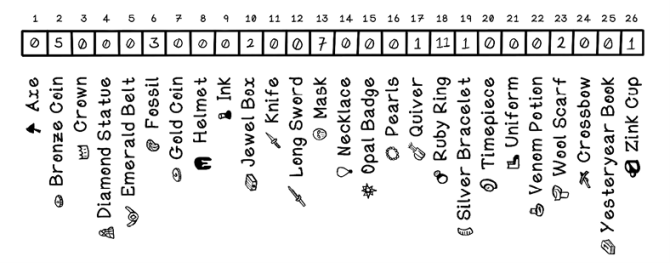
Figure 5.7 Example of real-value encoding

Because the encoding scheme has been changed, new crossover and mutation options become available. The crossover approaches discussed for binary encoding are still valid options to real-value encoding, but mutation should be approached differently.

Arithmetic crossover: Reproduce with math

Arithmetic crossover involves an arithmetic operation to be computed by using each parent as variables in the expression. The result of applying an arithmetic operation using both parents is the new offspring. When we use this strategy with binary encoding, it is important to ensure that the result of the operation is still a valid chromosome. Arithmetic crossover is applicable to binary encoding and real-value encoding (figure 5.8).

NOTE Be wary: this approach can create very diverse offspring, which can be problematic.

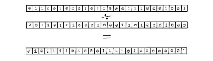
Figure 5.8 Example of arithmetic crossover

Boundary mutation

In boundary mutation, a gene randomly selected from a real-value encoded chromosome is set randomly to a lower bound value or upper bound value. Given 26 genes in a chromosome, a random index is selected, and the value is set to either a minimum value or a maximum value. In figure 5.9, the original value happens to be 0 and will be adjusted to 6, which is the maximum for that item. The minimum and maximum can be the same for all indexes or set uniquely for each index if knowledge of the problem informs the decision. This approach attempts to evaluate the impact of individual genes on the chromosome.

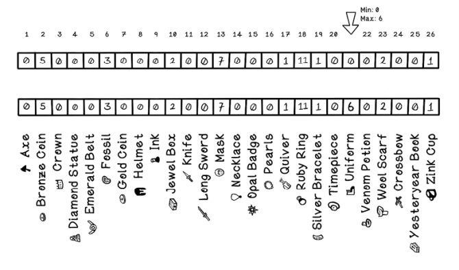
Figure 5.9 Example of boundary mutation

Arithmetic mutation

In arithmetic mutation, a randomly selected gene in a real-value-encoded chromosome is changed by adding or subtracting a small number. Note that although the example in figure 5.10 includes whole numbers, the numbers could be decimal numbers, including fractions.

Figure 5.10 Example of arithmetic mutation

Order encoding: Working with sequences

We still have the same items as in the Knapsack Problem. We won’t be determining the items that will fit into a knapsack; instead, all the items need to be processed in a refinery in which each item is broken down to extract its source material. Perhaps the gold coin, silver bracelet, and other items are smelted to extract only the source compounds. In this scenario, items are not selected to be included, but all are included.

To make things interesting, the refinery requires a steady rate of extraction, given the extraction time and the value of the item. It’s assumed that the value of the refined material is more or less the same as the value of the item. The problem becomes an ordering problem. In what order should the items be processed to maintain a constant rate of value? Table 5.2 describes the items with their respective extraction times.

Table 5.2 Factory value per hour: 600,000

Item ID	Item name	Weight (kg)	Value ($)	Extraction time
1	Axe	32,252	68,674	60
2	Bronze coin	225,790	471,010	30
3	Crown	468,164	944,620	45
4	Diamond statue	489,494	962,094	90
5	Emerald belt	35,384	78,344	70
6	Fossil	265,590	579,152	20
7	Gold coin	497,911	902,698	15
8	Helmet	800,493	1,686,515	20
9	Ink	823,576	1,688,691	10
10	Jewel box	552,202	1,056,157	40
11	Knife	323,618	677,562	15
12	Long sword	382,846	833,132	60
13	Mask	44,676	99,192	10
14	Necklace	169,738	376,418	20
15	Opal badge	610,876	1,253,986	60
16	Pearls	854,190	1,853,562	25
17	Quiver	671,123	1,320,297	30
18	Ruby ring	698,180	1,301,637	70
19	Silver bracelet	446,517	859,835	50
20	Timepiece	909,620	1,677,534	45
21	Uniform	904,818	1,910,501	5
22	Venom potion	730,061	1,528,646	5
23	Wool scarf	931,932	1,827,477	5
24	Crossbow	952,360	2,068,204	25
25	Yesteryear book	926,023	1,746,556	5
26	Zinc cup	978,724	2,100,851	10

Importance of the fitness function

With the change in the Knapsack Problem to the Refinery Problem, a key difference is the measurement of successful solutions. Because the factory requires a constant minimum rate of value per hour, the accuracy of the fitness function used becomes paramount to finding optimal solutions. In the Knapsack Problem, the fitness of a solution is trivial to compute, as it involves only two things: ensuring that the knapsack’s weight limit is respected and summing the selected items’ value. In the Refinery Problem, the fitness function must calculate the rate of value provided, given the extraction time for each item as well as the value of each item. This calculation is more complex, and an error in the logic of this fitness function directly influences the quality of solutions.

Order encoding at its core

Order encoding, also known as permutation encoding, represents a chromosome as a sequence of elements. Order encoding usually requires all elements to be present in the chromosome, which implies that corrections might need to be made when performing crossover and mutation to ensure that no elements are missing or duplicated. Figure 5.11 depicts how a chromosome represents the order of processing of the available items.

Figure 5.11 Example of order encoding

Another example in which order encoding is sensible is representing potential solutions to route optimization problems. Given a certain number of destinations, each of which must be visited at least once while minimizing the total distance traveled, the route can be represented as a string of the destinations in the order in which they are visited. We will use this example when covering swarm intelligence in chapter 6.

Order mutation: Order/permutation encoding

In order mutation, two randomly selected genes in an order-encoded chromosome swap positions, ensuring that all items remain in the chromosome while introducing diversity (figure 5.12).

Figure 5.12 Example of order mutation

Tree encoding: Working with hierarchies

The preceding sections show that binary encoding is useful for selecting items from a set, real-value encoding is useful when real numbers are important to the solution, and order encoding is useful for determining priority and sequences. Suppose that the items in the Knapsack Problem are placed in packages to be shipped to homes around the town. Each delivery wagon can hold a specific volume. The requirement is to determine the optimal positioning of packages to minimize empty space in each wagon (table 5.3).

Table 5.3 Wagon capacity: 1000 wide × 1000 high

Item ID	Item name	Weight (kg)	Value ($)	W	H
1	Axe	32,252	68,674	20	60
2	Bronze coin	225,790	471,010	10	10
3	Crown	468,164	944,620	20	20
4	Diamond statue	489,494	962,094	30	70
5	Emerald belt	35,384	78,344	30	20
6	Fossil	265,590	579,152	15	15
7	Gold coin	497,911	902,698	10	10
8	Helmet	800,493	1,686,515	40	50
9	Ink	823,576	1,688,691	5	10
10	Jewel box	552,202	1,056,157	40	30
11	Knife	323,618	677,562	10	30
12	Long sword	382,846	833,132	15	50
13	Mask	44,676	99,192	20	30
14	Necklace	169,738	376,418	15	20
15	Opal badge	610,876	1,253,986	5	5
16	Pearls	854,190	1,853,562	10	5
17	Quiver	671,123	1,320,297	30	70
18	Ruby ring	698,180	1,301,637	5	10
19	Silver bracelet	446,517	859,835	10	20
20	Timepiece	909,620	1,677,534	15	20
21	Uniform	904,818	1,910,501	30	40
22	Venom potion	730,061	1,528,646	15	15
23	Wool scarf	931,932	1,827,477	20	30
24	Crossbow	952,360	2,068,204	50	70
25	Yesteryear book	926,023	1,746,556	25	30
26	Zinc cup	978,724	2,100,851	15	25

In the interest of simplicity, suppose that the wagon’s volume is a two-dimensional rectangle and that the packages are rectangular rather than 3D boxes.

Tree encoding at its core

Tree encoding represents a chromosome as a tree of elements. Tree encoding is versatile for representing potential solutions in which the hierarchy of elements is important and/or required. Tree encoding can even represent functions, which consist of a tree of expressions. As a result, tree encoding could be used to evolve program functions in which the function solves a specific problem; the solution may work but look bizarre.

Here is an example in which tree encoding makes sense. We have a wagon with a specific height and width, and a certain number of packages must fit in the wagon. The goal is to fit the packages in the wagon so that empty space is minimized. A tree-encoding approach would work well in representing potential solutions to this problem.

In figure 5.13, the root node, node A, represents the packing of the wagon from top to bottom. Node B represents all packages horizontally, similarly to node C and node D. Node E represents packages packed vertically in its slice of the wagon.

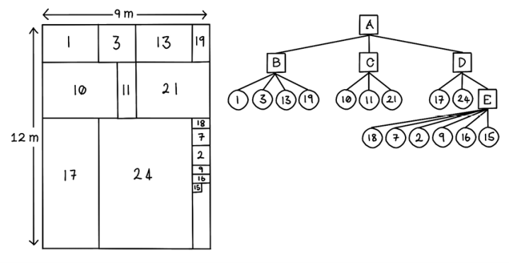
Figure 5.13 Example of a tree used to represent the Wagon Packing Problem

Tree crossover: Inheriting portions of a tree

Tree crossover is similar to single-point crossover (chapter 4) in that a single point in the tree structure is selected and then the parts are exchanged and combined with copies of the parent individuals to create an offspring individual. The inverse process can be used to make a second offspring. The resulting children must be verified to be valid solutions that obey the constraints of the problem. More than one point can be used for crossover if using multiple points makes sense in solving the problem (figure 5.14).

Figure 5.14 Example of tree crossover

Change node mutation: Changing the value of a node

In change node mutation, a randomly selected node in a tree-encoded chromosome is changed to a randomly selected valid object for that node. Given a tree representing an organization of items, we can change an item to another valid item (figure 5.15).

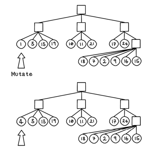
Figure 5.15 Change node mutation in a tree

This chapter and chapter 4 cover several encoding schemes, crossover schemes, and selection strategies. You could substitute your own approaches for these steps in your genetic algorithms if doing so makes sense for the problem you’re solving.

Common types of evolutionary algorithms

This chapter focuses on the life cycle and alternative approaches for a genetic algorithm. Variations of the algorithm can be useful for solving different problems. Now that we have a grounding in how a genetic algorithm works, we’ll look at these variations and possible use cases for them.

Genetic programming

Genetic programming follows a process similar to that of genetic algorithms but is used primarily to generate computer programs to solve problems. The process described in the previous section also applies here. The fitness of potential solutions in a genetic programming algorithm is how well the generated program solves a computational problem. With this in mind, we see that the tree-encoding method would work well here, because most computer programs are graphs consisting of nodes that indicate operations and processes. These trees of logic can be evolved, so the computer program will be evolved to solve a specific problem. One thing to note: these computer programs usually evolve to look like a mess of code that’s difficult for people to understand and debug.

Evolutionary programming

Evolutionary programming is similar to genetic programming, but the potential solution is parameters for a predefined fixed computer program, not a generated computer program. If a program requires finely tuned inputs, and determining a good combination of inputs is difficult, a genetic algorithm can be used to evolve these inputs. The fitness of potential solutions in an evolutionary programming algorithm is determined by how well the fixed computer program performs based on the parameters encoded in an individual. Perhaps an evolutionary programming approach could be used to find good parameters for an artificial neural network (chapter 9).

Glossary of evolutionary algorithm terms

Here is a useful glossary of evolutionary algorithms terms for future research and learning:

• Allele—The value of a specific gene in a chromosome

• Chromosome—A collection of genes that represents a possible solution

• Individual—A single chromosome in a population

• Population—A collection of individuals

• Genotype—The artificial representation of the potential solution population in the computation space

• Phenotype—The actual representation of the potential solution population in the real world

• Generation—A single iteration of the algorithm

• Exploration—The process of finding a variety of possible solutions, some of which may be good and some of which may be bad

• Exploitation—The process of honing in on good solutions and iteratively refining them

• Fitness function—A particular type of objective function

• Objective function—A function that attempts to maximize or minimize

More use cases for evolutionary algorithms

Some of the use cases for evolutionary algorithms are listed in chapter 4, but many more exist. The following use cases are particularly interesting because they use one or more of the concepts discussed in this chapter:

• Adjusting weights in artificial neural networks—Artificial neural networks are discussed later, in chapter 9, but a key concept is adjusting weights in the network to learn patterns and relationships in data. Several mathematical techniques adjust weights, but evolutionary algorithms are more efficient alternatives in the right scenarios.

• Electronic circuit design—Electronic circuits with the same components can be designed in many configurations. Some configurations are more efficient than others. If two components that work together often are closer together, this configuration may improve efficiency. Evolutionary algorithms can be used to evolve different circuit configurations to find the most optimal design.

• Molecular structure simulation and design—As in electronic circuit design, different molecules behave differently and have their own advantages and disadvantages. Evolutionary algorithms can be used to generate different molecular structures to be simulated and studied to determine their behavioral properties.

Now that we’ve been through the general genetic algorithm life cycle in chapter 4 and some advanced approaches in this chapter, you should be equipped to apply evolutionary algorithms in your contexts and solutions.

Summary of advanced evolutionary approaches