This chapter covers

• Understanding the inspiration for reinforcement learning

• Identifying problems to solve with reinforcement learning

• Designing and implementing a reinforcement learning algorithm

• Understanding reinforcement learning approaches

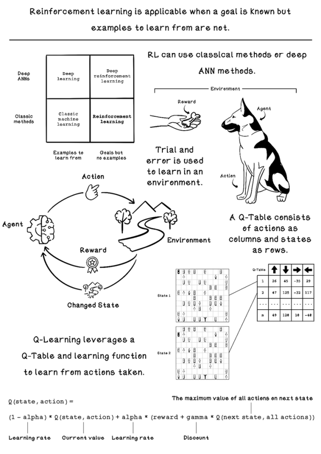
What is reinforcement learning?

Reinforcement learning (RL) is an area of machine learning inspired by behavioral psychology. The concept of reinforcement learning is based on cumulative rewards or penalties for the actions that are taken by an agent in a dynamic environment. Think about a young dog growing up. The dog is the agent in an environment that is our home. When we want the dog to sit, we usually say, “Sit.” The dog doesn’t understand English, so we might nudge it by lightly pushing down on its hindquarters. After it sits, we usually pet the dog or give it a treat. This process will need to be repeated several times, but after some time, we have positively reinforced the idea of sitting. The trigger in the environment is saying “Sit”; the behavior learned is sitting; and the reward is pets or treats.

Reinforcement learning is another approach to machine learning alongside supervised learning and unsupervised learning. Whereas supervised learning uses labeled data to make predictions and classifications, and unsupervised learning uses unlabeled data to find clusters and trends, reinforcement learning uses feedback from actions performed to learn what actions or sequence of actions are more beneficial in different scenarios toward an ultimate goal. Reinforcement learning is useful when you know what the goal is but don’t know what actions are reasonable to achieve it. Figure 10.1 shows the map of machine learning concepts and how reinforcement learning fits in.

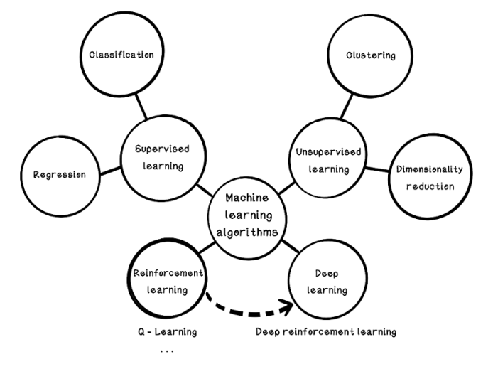
Figure 10.1 How reinforcement learning fits into machine learning

Reinforcement learning can be achieved through classical techniques or deep learning involving artificial neural networks. Depending on the problem being solved, either approach may be better.

Figure 10.2 illustrates when different machine learning approaches may be used. We will be exploring reinforcement learning through classical methods in this chapter.

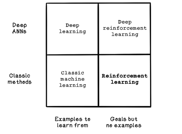
Figure 10.2 Categorization of machine learning, deep learning, and reinforcement learning

The inspiration for reinforcement learning

Reinforcement learning in machines is derived from behavioral psychology, a field that is interested in the behavior of humans and other animals. Behavioral psychology usually explains behavior by a reflex action, or something learned in the individual’s history. The latter includes exploring reinforcement through rewards or punishments, motivators for behaviors, and aspects of the individual’s environment that contribute to the behavior.

Trial and error is one of the most common ways that most evolved animals learn what is beneficial to them and what is not. Trial and error involves trying something, potentially failing at it, and trying something different until you succeed. This process may happen many times before a desired outcome is obtained, and it’s largely driven by some reward.

This behavior can be observed throughout nature. Newborn chicks, for example, try to peck any small piece of material that they come across on the ground. Through trial and error, the chicks learn to peck only food.

Another example is chimpanzees learning through trial and error that using a stick to dig the soil is more favorable than using their hands. Goals, rewards, and penalties are important in reinforcement learning. A goal for a chimpanzee is to find food; a reward or penalty may be the number of times it has dug a hole or the time taken to dig a hole. The faster it can dig a hole, the faster it will find some food.

Figure 10.3 looks at the terminology used in reinforcement learning with reference to the simple dog-training example.

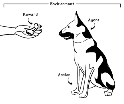
Figure 10.3 Example of reinforcement learning: teaching a dog to sit by using food as a reward

Reinforcement learning has negative and positive reinforcement. Positive reinforcement is receiving a reward after performing an action, such as a dog getting a treat after it sits. Negative reinforcement is receiving a penalty after performing an action, such as a dog getting scolded after it tears up a carpet. Positive reinforcement is meant to motivate desired behavior, and negative reinforcement is meant to discourage undesired behavior.

Another concept in reinforcement learning is balancing instant gratification with long-term consequences. Eating a chocolate bar is great for getting a boost of sugar and energy; this is instant gratification. But eating a chocolate bar every 30 minutes will likely cause health problems later in life; this is a long-term consequence. Reinforcement learning aims to maximize the long-term benefit over short-term benefit, although short-term benefit may contribute to long-term benefit.

Reinforcement learning is concerned with the long-term consequence of actions in an environment, so time and the sequence of actions are important. Suppose that we’re stranded in the wilderness, and our goal is to survive as long as possible while traveling as far as possible in hopes of finding safety. We’re positioned next to a river and have two options: jump into the river to travel downstream faster or walk along the side of the river. Notice the boat on the side of the river in figure 10.4. By swimming, we will travel faster but might miss the boat by being dragged down the wrong fork in the river. By walking, we will be guaranteed to find the boat, which will make the rest of the journey much easier, but we don’t know this at the start. This example shows how important the sequence of actions is in reinforcement learning. It also shows how instant gratification may lead to long-term detriment. Furthermore, in a landscape that didn’t contain a boat, the consequence of swimming is that we will travel faster but have soaked clothing, which may be problematic when it gets cold. The consequence of walking is that we will travel slower but not wet our clothing, which highlights the fact that a specific action may work in one scenario but not in others. Learning from many simulation attempts is important to finding more-generalist approaches.

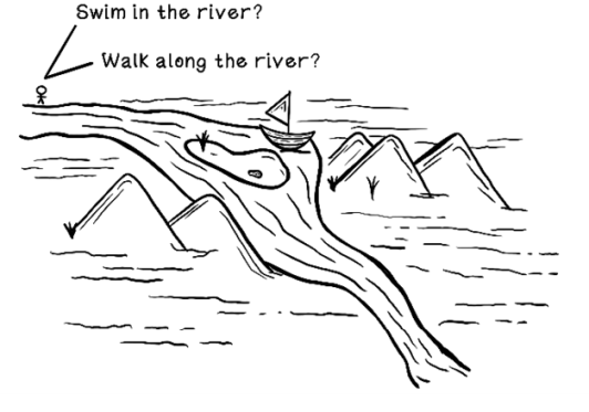
Figure 10.4 An example of possible actions that have long-term consequences

Problems applicable to reinforcement learning

To sum it up, reinforcement learning aims to solve problems in which a goal is known but the actions required to achieve it are not. These problems involve controlling an agent’s actions in an environment. Individual actions may be rewarded more than others, but the main concern is the cumulative reward of all actions.

Reinforcement learning is most useful for problems in which individual actions build up toward a greater goal. Areas such as strategic planning, industrial-process automation, and robotics are good cases for the use of reinforcement learning. In these areas, individual actions may be suboptimal to gain a favorable outcome. Imagine a strategic game such as chess. Some moves may be poor choices based on the current state of the board, but they help set the board up for a greater strategic win later in the game. Reinforcement learning works well in domains in which chains of events are important for a good solution.

To work through the steps in a reinforcement learning algorithm, we will use the example car-collision problem from chapter 9 as inspiration. This time, however, we will be working with visual data about a self-driving car in a parking lot trying to navigate to its owner. Suppose that we have a map of a parking lot, including a self-driving car, other cars, and pedestrians. Our self-driving car can move north, south, east, and west. The other cars and pedestrians remain stationary in this example.

The goal is for our car to navigate the road to its owner while colliding with as few cars and pedestrians as possible—ideally, not colliding with anything. Colliding with a car is not good because it damages the vehicles, but colliding with a pedestrian is more severe. In this problem, we want to minimize collisions, but if we have a choice between colliding with a car and a pedestrian, we should choose the car. Figure 10.5 depicts this scenario.

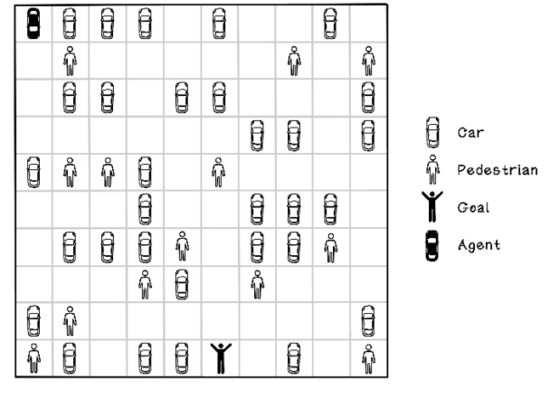
Figure 10.5 The self-driving car in a parking lot problem

We will be using this example problem to explore the use of reinforcement learning for learning good actions to take in dynamic environments.

The life cycle of reinforcement learning

Like other machine learning algorithms, a reinforcement learning model needs to be trained before it can be used. The training phase centers on exploring the environment and receiving feedback, given specific actions performed in specific circumstances or states. The life cycle of training a reinforcement learning model is based on the Markov Decision Process, which provides a mathematical framework for modeling decisions (figure 10.6). By quantifying decisions made and their outcomes, we can train a model to learn what actions toward a goal are most favorable.

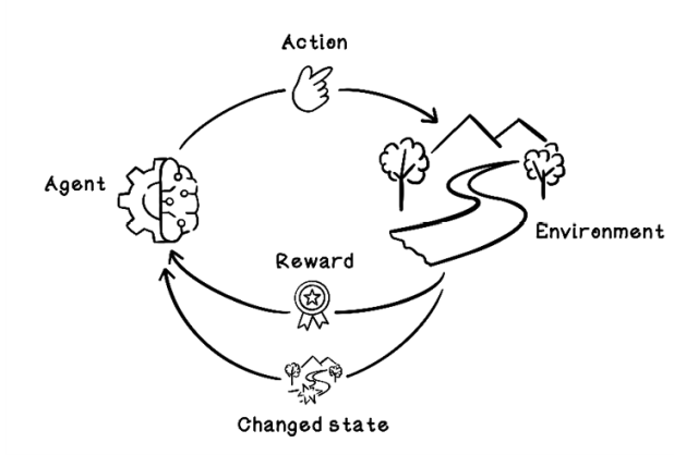
Figure 10.6 The Markov Decision Process for reinforcement learning

Before we can start tackling the challenge of training a model by using reinforcement learning, we need an environment that simulates the problem space we are working in. Our example problem entails a self-driving car trying to navigate a parking lot filled with obstacles to find its owner while avoiding collisions. This problem needs to be modeled as a simulation so that actions in the environment can be measured toward the goal. This simulated environment is different from the model that will learn what actions to take.

Simulation and data: Make the environment come alive

Figure 10.7 depicts a parking-lot scenario containing several other cars and pedestrians. The starting position of the self-driving car and the location of its owner are represented as black figures. In this example, the self-driving car that applies actions to the environment is known as the agent.

The self-driving car, or agent, can take several actions in the environment. In this simple example, the actions are moving north, south, east, and west. Choosing an action results in the agent moving one block in that direction. The agent can’t move diagonally.

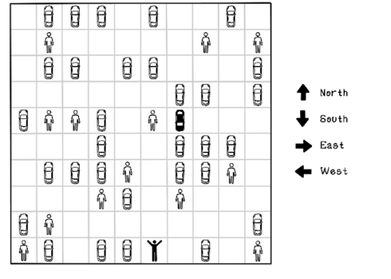
Figure 10.7 Agent actions in the parking-lot environment

When actions are taken in the environment, rewards or penalties occur. Figure 10.8 shows the reward points awarded to the agent based on the outcome in the environment. A collision with another car is bad; a collision with a pedestrian is terrible. A move to an empty space is good; finding the owner of the self-driving car is better. The specified rewards aim to discourage collisions with other cars and pedestrians, and to encourage moving into empty spaces and reaching the owner. Note that there could be a reward for out-of-bounds movements, but we will simply disallow this possibility for the sake of simplicity.

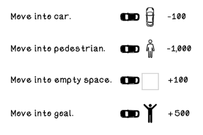
Figure 10.8 Rewards due to specific events in the environment due to actions performed

NOTE An interesting outcome of the rewards and penalties described is that the car may drive forward and backward on empty spaces indefinitely to accumulate rewards. We will dismiss this as a possibility for this example, but it highlights the importance of crafting good rewards.

The simulator needs to model the environment, the actions of the agent, and the rewards received after each action. A reinforcement learning algorithm will use the simulator to learn through practice by taking actions in the simulated environment and measuring the outcome. The simulator should provide the following functionality and information at minimum:

• Initialize the environment. This function involves resetting the environment, including the agent, to the starting state.

• Get the current state of the environment. This function should provide the current state of the environment, which will change after each action is performed.

• Apply an action to the environment. This function involves having the agent apply an action to the environment. The environment is affected by the action, which may result in a reward.

• Calculate the reward of the action. This function is related to applying the action to the environment. The reward for the action and effect on the environment need to be calculated.

• Determine whether the goal is achieved. This function determines whether the agent has achieved the goal. The goal can also sometimes be represented as is complete. In an environment in which the goal cannot be achieved, the simulator needs to signal completion when it deems necessary.

Figures 10.9 and 10.10 depict possible paths in the self-driving-car example. In figure 10.9, the agent travels south until it reaches the boundary; then it travels east until it reaches the goal. Although the goal is achieved, the scenario resulted in five collisions with other cars and one collision with a pedestrian—not an ideal result. Figure 10.10 depicts the agent traveling along a more specific path toward the goal, resulting in no collisions, which is great. It’s important to note that given the rewards that we have specified, the agent is not guaranteed to achieve the shortest path; because we heavily encourage avoiding obstacles, the agent may find any path that is obstacle-free.

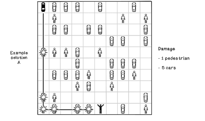
Figure 10.9 A bad solution to the parking-lot problem

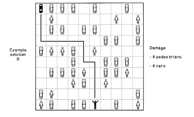
Figure 10.10 A good solution to the parking-lot problem

At this moment, there is no automation in sending actions to the simulator. It’s like a game in which we provide input as a person instead of an AI providing the input. The next section explores how to train an autonomous agent.

Pseudocode

The pseudocode for the simulator encompasses the functions discussed in this section. The simulator class would be initialized with the information relevant to the starting state of the environment.

The move_agent function is responsible for moving the agent north, south, east, or west, based on the action. It determines whether the movement is within bounds, adjusts the agent’s coordinates, determines whether a collision occurred, and returns a reward score based on the outcome:

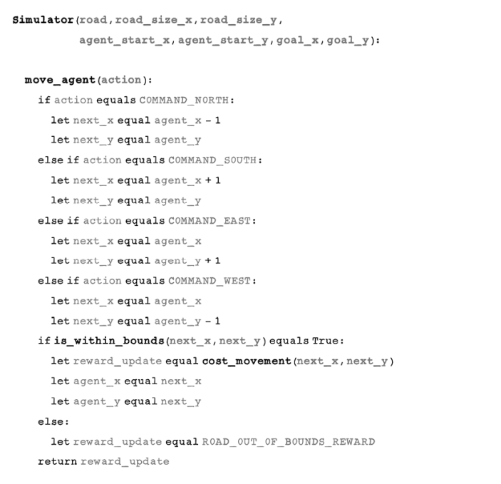
Here are descriptions of the next functions in the pseudocode:

• The cost_movement function determines the object in the target coordinate that the agent will move to and returns the relevant reward score.

• The is_within_bounds function is a utility function that makes sure the target coordinate is within the boundary of the road.

• The is_goal_achieved function determines whether the goal has been found, in which case the simulation can end.

• The get_state function uses the agent’s position to determine a number that enumerates the current state. Each state must be unique. In other problem spaces, the state may be represented by the actual native state itself.

Training with the simulation using Q-learning

Q-learning is an approach in reinforcement learning that uses the states and actions in an environment to model a table that contains information describing favorable actions based on specific states. Think of Q-learning as a dictionary in which the key is the state of the environment and the value is the best action to take for that state.

Reinforcement learning with Q-learning employs a reward table called a Q-table. A Q-table consists of columns that represent the possible actions and rows that represent the possible states in the environment. The point of a Q-table is to describe which actions are most favorable for the agent as it seeks a goal. The values that represent favorable actions are learned through simulating the possible actions in the environment and learning from the outcome and change in state. It’s worth noting that the agent has a chance of choosing a random action or an action from the Q-table, as shown later in figure 10.13. The Q represents the function that provides the reward, or quality, of an action in an environment.

Figure 10.11 depicts a trained Q-table and two possible states that may be represented by the action values for each state. These states are relevant to the problem we’re solving; another problem might allow the agent to move diagonally as well. Note that the number of states differs based on the environment and that new states can be added as they are discovered. In state 1, the agent is in the top-left corner, and in state 2, the agent is in the position below its previous state. The Q-table encodes the best actions to take, given each respective state. The action with the largest number is the most beneficial action. In this figure, the values in the Q-table have already been found through training. Soon, we will see how they’re calculated.

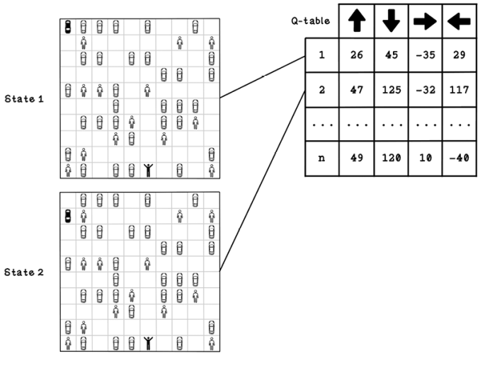
Figure 10.11 An example Q-table and states that it represents

The big problem with representing the state using the entire map is that the configuration of other cars and people is specific to this problem. The Q-table learns the best choices only for this map.

A better way to represent state in this example problem is to look at the objects adjacent to the agent. This approach allows the Q-table to adapt to other parking-lot configurations, because the state is less specific to the example parking lot from which it is learning. This approach may seem to be trivial, but a block could contain another car or a pedestrian, or it could be an empty block or an out-of-bounds block, which works out to four possibilities per block, resulting in 65,536 possible states. With this much variety, we would need to train the agent in many parking-lot configurations many times for it to learn good short-term action choices (figure 10.12).

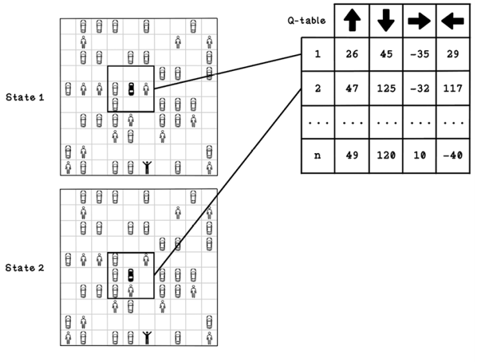
Figure 10.12 A better example of a Q-table and states that it represents

Keep the idea of a reward table in mind as we explore the life cycle of training a model using reinforcement learning with Q-learning. It will represent the model for actions that the agent will take in the environment.

Let’s take a look at the life cycle of a Q-learning algorithm, including the steps involved in training. We will look at two phases: initialization, and what happens over several iterations as the algorithm learns (figure 10.13):

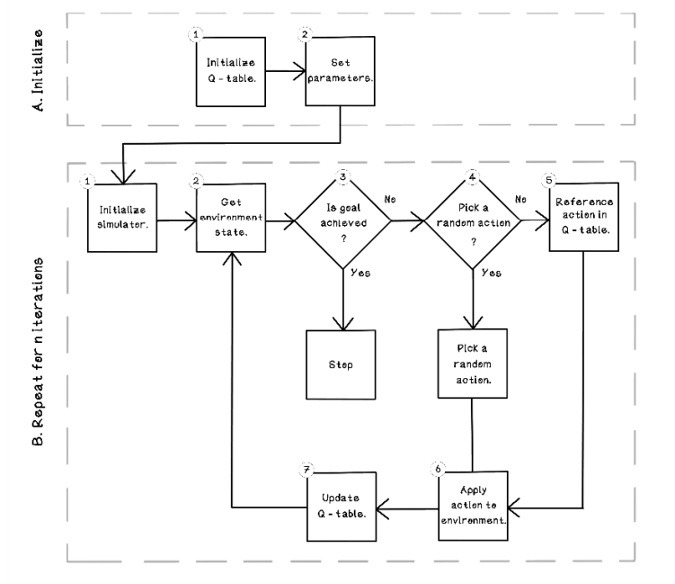
Figure 10.13 Life cycle of a Q-learning reinforcement learning algorithm

• Initialize. The initialize step involves setting up the relevant parameters and initial values for the Q-table:

  1. Initialize Q-table. Initialize a Q-table in which each column is an action and each row represents a possible state. Note that states can be added to the table as they are encountered, because it can be difficult to know the number of states in the environment at the beginning. The initial action values for each state are initialized with 0s.

  2. Set parameters. This step involves setting the parameters for different hyperparameters of the Q-learning algorithm, including:

     • Chance of choosing a random action—This is the value threshold for choosing a random action over choosing an action from the Q-table.
     • Learning rate—The learning rate is similar to the learning rate in supervised learning. It describes how quickly the algorithm learns from rewards in different states. With a high learning rate, values in the Q-table change erratically, and with a low learning rate, the values change gradually but it will potentially take more iterations to find good values.
     • Discount factor—The discount factor describes how much potential future rewards are valued, which translates to favoring immediate gratification or long-term reward. A small value favors immediate rewards; a large value favors long-term rewards.

• Repeat for n iterations. The following steps are repeated to find the best actions in the same states by evaluating these states multiple times. The same Q-table will be updated over all iterations. The key concept is that because the sequence of actions for an agent is important, the reward for an action in any state may change based on previous actions. For this reason, multiple iterations are important. See an iteration as a single attempt to achieving a goal:

  1. Initialize simulator. This step involves resetting the environment to the starting state, with the agent in a neutral state.

  2. Get environment state. This function should provide the current state of the environment. The state of the environment will change after each action is performed.

  3. Is goal achieved? Determine whether the goal is achieved (or the simulator deems the exploration to be complete). In our example, this goal is picking up the owner of the self-driving car. If the goal is achieved, the algorithm ends.

  4. Pick a random action. Determine whether a random action should be selected. If so, a random action will be selected (north, south, east, or west). Random actions are useful for exploring the possibilities in the environment instead of learning a narrow subset.

  5. Reference action in Q-table. If the decision to select a random action is not selected, the current environment state is transposed to the Q-table, and the respective action is selected based on the values in the table. More about the Q-table is coming up.

  6. Apply action to environment .This step involves applying the selected action to the environment, whether that action is random or one selected from the Q-table. An action will have a consequence in the environment and yield a reward.

  7. Update Q-table. The following material describes the concepts involved in updating the Q-table and the steps that are carried out.

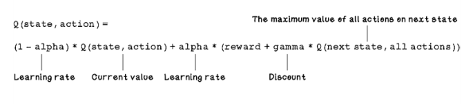
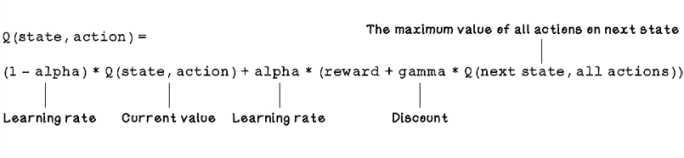
The key aspect of Q-learning is the equation used to update the values of the Q-table. This equation is based on the Bellman equation, which determines the value of a decision made at a certain point in time, given the reward or penalty for making that decision. The Q-learning equation is an adaptation of the Bellman equation. In the Q-learning equation, the most important properties for updating Q-table values are the current state, the action, the next state given the action, and the reward outcome. The learning rate is similar to the learning rate in supervised learning, which determines the extent to which a Q-table value is updated. The discount is used to indicate the importance of possible future rewards, which is used to balance favoring immediate rewards versus long-term rewards:

Because the Q-table is initialized with 0s, it looks similar to figure 10.14 in the initial state of the environment.

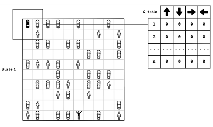
Figure 10.14 An example initialized Q-table

Next, we explore how to update the Q-table by using the Q-learning equation based on different actions with different reward values. These values will be used for the learning rate (alpha) and discount (gamma):

• Learning rate (alpha): 0.1

• Discount (gamma): 0.6

Figure 10.15 illustrates how the Q-learning equation is used to update the Q-table, if the agent selects the East action from the initial state in the first iteration. Remember that the initial Q-table consists of 0s. The learning rate (alpha), discount (gamma), current action value, reward, and next best state are plugged into the equation to determine the new value for the action that was taken. The action is East, which results in a collision with another car, which yields -100 as a reward. After the new value is calculated, the value of East on state 1 is -10.

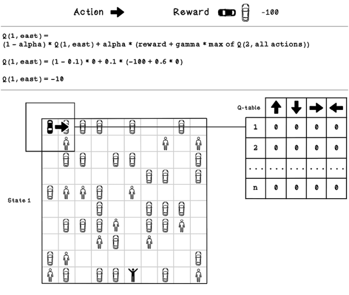
Figure 10.15 Example Q-table update calculation for state 1

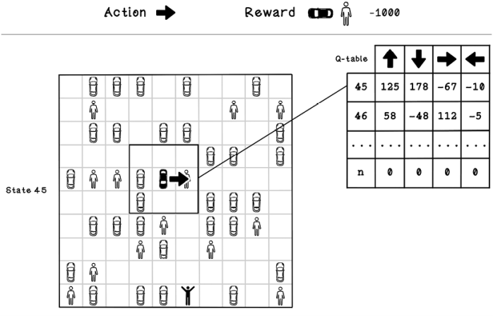
The next calculation is for the next state in the environment following the action that was taken. The action is South and results in a collision with a pedestrian, which yields -1,000 as the reward. After the new value is calculated, the value for the South action on state 2 is -100 (figure 10.16).

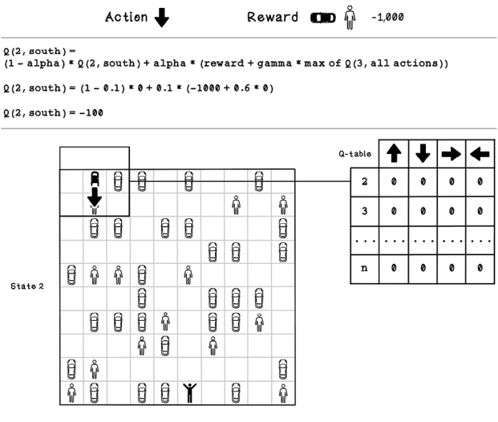
Figure 10.16 Example Q-table update calculation for state 2

Figure 10.17 illustrates how the calculated values differ in a Q-table with populated values because we worked on a Q-table initialized with 0s. The figure is an example of the Q-learning equation updated from the initial state after several iterations. The simulation can be run multiple times to learn from multiple attempts. So, this iteration is succeeding many before it, where the values of the table have been updated. The action for East results in a collision with another car and yields -100 as a reward. After the new value is calculated, the value for East on state 1 changes to -34.

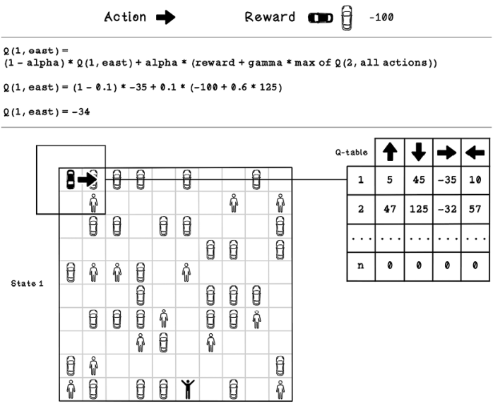
Figure 10.17 Example Q-table update calculation for state 1 after several iterations

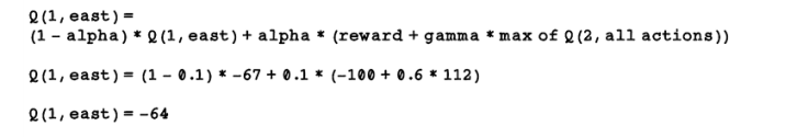
Exercise: Calculate the change in values for the Q-table

Using the Q-learning update equation and the following scenario, calculate the new value for the action performed. Assume that the last move was East with a value of -67:

Solution: Calculate the change in values for the Q-table

The hyperparameter and state values are plugged into the Q-learning equation, resulting in the new value for Q(1, east):

• Learning rate (alpha): 0.1
• Discount (gamma): 0.6
• Q(1, east): -67
• Max of Q(2, all actions): 112

Pseudocode

This pseudocode describes a function that trains a Q-table by using Q-learning. It could be broken into simpler functions but is represented this way for readability. The function follows the steps described in this chapter.

The Q-table is initialized with 0s; then the learning logic is run for several iterations. Remember that an iteration is an attempt to achieve the goal.

The next piece of logic runs while the goal has not been achieved:

1. Decide whether a random action should be taken to explore possibilities in the environment. If not, the highest value action for the current state is selected from the Q-table.

2. Proceed with the selected action, and apply it to the simulator.

3. Gather information from the simulator, including the reward, the next state given the action, and whether the goal is reached.

4. Update the Q-table based on the information gathered and hyperparameters. Note that in this code, the hyperparameters are passed through as arguments of this function.

5. Set the current state to the state outcome of the action just performed.

These steps will continue until a goal is found. After the goal is found and the desired number of iterations is reached, the result is a trained Q-table that can be used to test in other environments. We look at testing the Q-table in the next section:

Testing with the simulation and Q-table

We know that in the case of using Q-learning, the Q-table is the model that encompasses the learnings. When presented with a new environment with different states, the algorithm references the respective state in the Q-table and chooses the highest-valued action. Because the Q-table has already been trained, this process consists of getting the current state of the environment and referencing the respective state in the Q-table to find an action until a goal is achieved (figure 10.18).

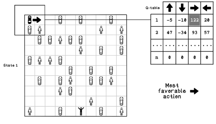
Figure 10.18 Referencing a Q-table to determine what action to take

Because the state learned in the Q-table considers the objects directly next to the agent’s current position, the Q-table has learned good and bad moves for short-term rewards, so the Q-table could be used in a different parking-lot configuration, such as the one shown in figure 10.18. The disadvantage is that the agent favors short-term rewards over long-term rewards because it doesn’t have the context of the rest of the map when taking each action.

One term that will likely come up in the process of learning more about reinforcement learning is episodes. An episode includes all the states between the initial state and the state when the goal is achieved. If it takes 14 actions to achieve a goal, we have 14 episodes. If the goal is never achieved, the episode is called infinite.

Measuring the performance of training

Reinforcement learning algorithms can be difficult to measure generically. Given a specific environment and goal, we may have different penalties and rewards, some of which have a greater effect on the problem context than others. In the parking-lot example, we heavily penalize collisions with pedestrians. In another example, we may have an agent that resembles a human and tries to learn what muscles to use to walk naturally as far as possible. In this scenario, penalties may be falling or something more specific, such as too-large stride lengths. To measure performance accurately, we need the context of the problem.

One generic way to measure performance is to count the number of penalties in a given number of attempts. Penalties could be events that we want to avoid that happen in the environment due to an action.

Another measurement of reinforcement learning performance is average reward per action. By maximizing the reward per action, we aim to avoid poor actions, whether the goal was reached or not. This measurement can be calculated by dividing the cumulative reward by the total number of actions.

Model-free and model-based learning

To support your future learning in reinforcement learning, be aware of two approaches for reinforcement learning: model-based and model-free, which are different from the machine learning models discussed in this book. Think of a model as being an agent’s abstract representation of the environment in which it is operating.

We may have a model in our heads about locations of landmarks, intuition of direction, and the general layout of the roads within a neighborhood. This model has been formed from exploring some roads, but we’re able to simulate scenarios in our heads to make decisions without trying every option. To decide how we will get to work, for example, we can use this model to make a decision; this approach is model-based. Model-free learning is similar to the Q-learning approach described in this chapter; trial and error is used to explore many interactions with the environment to determine favorable actions in different scenarios.

Figure 10.19 depicts the two approaches in road navigation. Different algorithms can be employed to build model-based reinforcement learning implementations.

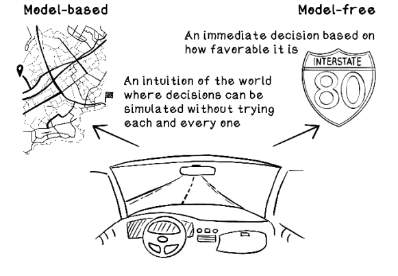
Figure 10.19 Examples of model-based and model-free reinforcement learning

Deep learning approaches to reinforcement learning

Q-learning is one approach to reinforcement learning. Having a good understanding of how it functions allows you to apply the same reasoning and general approach to other reinforcement learning algorithms. Several alternative approaches depend on the problem being solved. One popular alternative is deep reinforcement learning, which is useful for applications in robotics, video-game play, and problems that involve images and video.

Deep reinforcement learning can use artificial neural networks (ANNs) to process the states of an environment and produce an action. The actions are learned by adjusting weights in the ANN, using the reward feedback and changes in the environment. Reinforcement learning can also use the capabilities of convolutional neural networks (CNNs) and other purpose-built ANN architectures to solve specific problems in different domains and use cases.

Figure 10.20 depicts, at a high level, how an ANN can be used to solve the parking-lot problem in this chapter. The inputs to the neural network are the states; the outputs are probabilities for best action selection for the agent; and the reward and effect on the environment can be fed back using backpropagation to adjust the weights in the network.

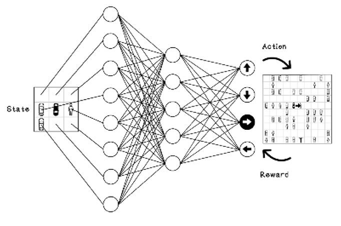
Figure 10.20 Example of using an ANN for the parking-lot problem

The next section looks at some popular use cases for reinforcement learning in the real world.

Use cases for reinforcement learning

Reinforcement learning has many applications where there is no or little historic data to learn from. Learning happens through interacting with an environment that has heuristics for good performance. Use cases for this approach are potentially endless. This section describes some popular use cases for reinforcement learning.

Robotics

Robotics involves creating machines that interact with real-world environments to accomplish goals. Some robots are used to navigate difficult terrain with a variety of surfaces, obstacles, and inclines. Other robots are used as assistants in a laboratory, taking instructions from a scientist, passing the right tools, or operating equipment. When it isn’t possible to model every outcome of every action in a large, dynamic environment, reinforcement learning can be useful. By defining a greater goal in an environment and introducing rewards and penalties as heuristics, we can use reinforcement learning to train robots in dynamic environments. A terrain-navigating robot, for example, may learn which wheels to drive power to and how to adjust its suspension to traverse difficult terrain successfully. This goal is achieved after many attempts.

These scenarios can be simulated virtually if the key aspects of the environment can be modeled in a computer program. Computer games have been used in some projects as a baseline for training self-driving cars before they’re trained on the road in the real world. The aim in training robots with reinforcement learning is to create more-general models that can adapt to new and different environments while learning more-general interactions, much the way that humans do.

Recommendation engines

Recommendation engines are used in many of the digital products we use. Video streaming platforms use recommendation engines to learn an individual’s likes and dislikes in video content and try to recommend something most suitable for the viewer. This approach has also been employed in music streaming platforms and e-commerce stores. Reinforcement learning models are trained by using the behavior of the viewer when faced with decisions to watch recommended videos. The premise is that if a recommended video was selected and watched in its entirety, there’s a strong reward for the reinforcement learning model, because it has assumed that the video was a good recommendation. Conversely, if a video never gets selected or little of the content is watched, it’s reasonable to assume that the video did not appeal to the viewer. This result would result in a weak reward or a penalty.

Financial trading

Financial instruments for trading include stock in companies, cryptocurrency, and other packaged investment products. Trading is a difficult problem. Analysts monitor patterns in price changes and news about the world, and use their judgment to make a decision to hold their investment, sell part of it, or buy more. Reinforcement learning can train models that make these decisions through rewards and penalties based on income made or loss incurred. Developing a reinforcement learning model to trade well takes a lot of trial and error, which means that large sums of money could be lost in training the agent. Luckily, most historic public financial data is freely available, and some investment platforms provide sandboxes to experiment with.

Although a reinforcement learning model could help generate a good return on investment, here’s an interesting question: if all investors were automated and completely rational, and the human element was removed from trading, what would the market look like?

Game playing

Popular strategy computer games have been pushing players’ intellectual capabilities for years. These games typically involve managing many types of resources while planning short-term and long-term tactics to overcome an opponent. These games have filled arenas, and the smallest mistakes have cost top-notch players many matches. Reinforcement learning has been used to play these games at the professional level and beyond. These reinforcement learning implementations usually involve an agent watching the screen the way a human player would, learning patterns, and taking actions. The rewards and penalties are directly associated with the game. After many iterations of playing the game in different scenarios with different opponents, a reinforcement learning agent learns what tactics work best toward the long-term goal of winning the game. The goal of research in this space is related to the search for more-general models that can gain context from abstract states and environments and understand things that cannot be mapped out logically. As children, for example, we never got burned by multiple objects before learning that hot objects are potentially dangerous. We developed an intuition and tested it as we grew older. These tests reinforced our understanding of hot objects and their potential harm or benefit.

In the end, AI research and development strives to make computers learn to solve problems in ways that humans are already good at: in a general way, stringing abstract ideas and concepts together with a goal in mind and finding good solutions to problems.

Summary of reinforcement learning