7 Swarm intelligence: Particles
-
Understanding the inspiration for particle swarm intelligence algorithms
-
Understanding and solving optimization problems
-
Designing and implementing a particle swarm optimization algorithm
What is particle swarm optimization?
Particle swarm optimization is another swarm algorithm. Swarm intelligence relies on emergent behavior of many individuals to solve difficult problems as a collective. We saw in chapter 6 how ants can find the shortest paths between destinations through their use of pheromones.
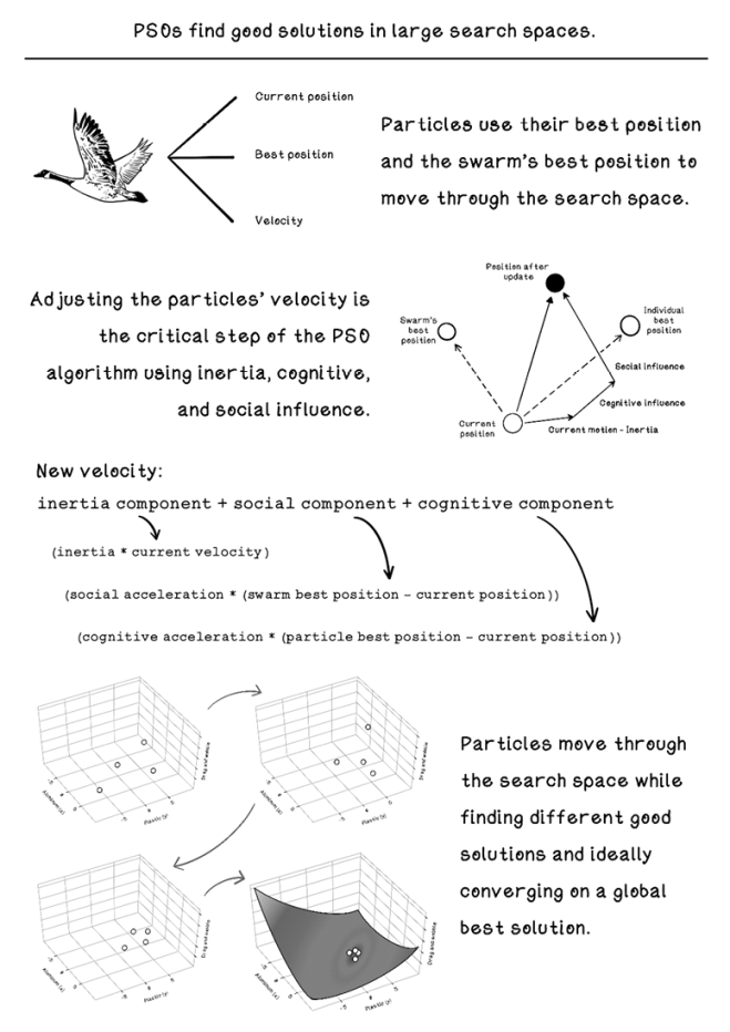
Bird flocks are another ideal example of swarm intelligence in nature. When a single bird is flying, it might attempt several maneuvers and techniques to preserve energy, such as jumping and gliding through the air or leveraging wind currents to carry it in the direction in which it intends to travel. This behavior indicates some primitive level of intelligence in a single individual. But birds also have the need to migrate during different seasons. In winter, there is less availability of insects and other food. Suitable nesting locations also become scarce. Birds tend to flock to warmer areas to take advantage of better weather conditions, which improves their likelihood of survival. Migration is usually not a short trip. It takes thousands of kilometers of movement to arrive at an area with suitable conditions. When birds travel these long distances, they tend to flock. Birds flock because there is strength in numbers when facing predators; additionally, it saves energy. The formation that we observe in bird flocks has several advantages. A large, strong bird will take the lead, and when it flaps its wings, it creates uplift for the birds behind it. These birds can fly while using significantly less energy. Flocks can change leaders if the direction changes or if the leader becomes fatigued. When a specific bird moves out of formation, it experiences more difficulty in flying via air resistance and corrects its movement to get back into formation. Figure 7.1 illustrates a bird flock formation; you may have seen something similar.

Figure 7.1 An example bird flock formation
Craig Reynolds developed a simulator program in 1987 to understand the attributes of emergent behavior in bird flocks and used the following rules to guide the group. These rules are extracted from observation of bird flocks:
-
Alignment—An individual should steer in the average heading of its neighbors to ensure that the group travels in a similar direction.
-
Cohesion—An individual should move toward the average position of its neighbors to maintain the formation of the group.
-
Separation—An individual should avoid crowding or colliding with its neighbors to ensure that individuals do not collide, disrupting the group.
Additional rules are used in different variants of attempting to simulate swarm behavior. Figure 7.2 illustrates the behavior of an individual in different scenarios, as well as the direction in which it is influenced to move to obey the respective rule. Adjusting movement is a balance of these three principles shown in the figure.
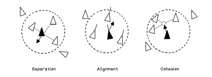
Figure 7.2 Rules that guide a swarm
Particle swarm optimization involves a group of individuals at different points in the solution space, all using real-life swarm concepts to find an optimal solution in the space. This chapter dives into the workings of the particle swarm optimization algorithm and shows how it can be used to solve problems. Imagine a swarm of bees that spreads out looking for flowers and gradually converges on an area that has the most density of flowers. As more bees find the flowers, more are attracted to the flowers. At its core, this example is what particle swarm optimization entails (figure 7.3).
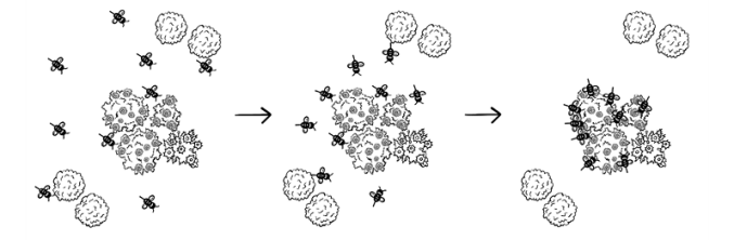
Figure 7.3 A bee swarm converging on its goal
Optimization problems have been mentioned in several chapters. Finding the optimal path through a maze, determining the optimal items for a knapsack, and finding the optimal path between attractions in a carnival are examples of optimization problems. We worked through them without diving into the details behind them. From this chapter on, however, a deeper understanding of optimization problems is important. The next section works through some of the intuition to be able to spot optimization problems when they occur.
Optimization problems: A slightly more technical perspective
Suppose that we have several peppers of different sizes. Usually, small peppers tend to be spicier than large peppers. If we plot all the peppers on a chart based on size and spiciness, it may look like figure 7.4.
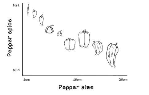
Figure 7.4 Pepper spice vs. pepper size
The figure depicts the size of each pepper and how spicy it is. Now, by removing the imagery of the peppers, plotting the data points, and drawing a possible curve between them, we are left with figure 7.5. If we had more peppers, we would have more data points, and the curve would be more accurate.
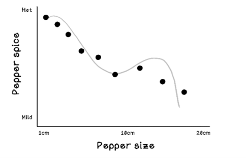
Figure 7.5 Pepper spice vs. pepper size trend
This example could potentially be an optimization problem. If we searched for a minimum from left to right, we would come across several points less than the previous ones, but in the middle, we encounter one that is higher. Should we stop? If we did, we would be missing the actual minimum, which is the last data point, known as the global minimum.
The trend line/curve that is approximated can be represented by a function, such as the one shown in figure 7.6. This function can be interpreted as the spiciness of the pepper being equal to the result of this function where the size of the pepper is represented by x.

Figure 7.6 An example function for pepper spice vs. pepper size
Real-world problems typically have thousands of data points, and the minimum output of the function is not as clear as this example. The search spaces are massive and difficult to solve by hand.
Notice that we have used only two properties of the pepper to create the data points, which resulted in a simple curve. If we consider another property of the pepper, such as color, the representation of the data changes significantly. Now the chart has to be represented in 3D, and the trend becomes a surface instead of a curve. A surface is like a warped blanket in three dimensions (figure 7.7). This surface is also represented as a function but is more complex.

Figure 7.7 Pepper spice vs. pepper size vs. pepper color
Furthermore, a 3D search space could look fairly simple, like figure 7.7, or be so complex that attempting to inspect it visually to find the minimum would be almost impossible (figure 7.8).

Figure 7.8 A function visualized in the 3D space as a plane
Figure 7.9 shows the function that represents this plane.

Figure 7.9 The function that represents the surface in figure 7.8
It gets more interesting! We have looked at three attributes of a pepper: its size, its color, and how spicy it is. As a result, we’re searching in three dimensions. What if we want to include the location of growth? This attribute would make it even more difficult to visualize and understand the data, because we are searching in four dimensions. If we add the pepper’s age and the amount of fertilizer used while growing it, we are left with a massive search space in six dimensions, and we can’t imagine what this search might look like. This search too is represented by a function, but again, it is too complex and difficult for a person to solve.
Particle swarm optimization algorithms are particularly good at solving difficult optimization problems. Particles are distributed over the multidimensional search space and work together to find good maximums or minimums.
Particle swarm optimization algorithms are particularly useful in the following scenarios:
-
Large search spaces—There are many data points and possibilities of combinations.
-
Search spaces with high dimensions—There is complexity in high dimensions. Many dimensions of a problem are required to find a good solution.
Exercise: How many dimensions will the search space for the following scenario be?
In this scenario, we need to determine a good city to live in based on the average minimum temperature during the year, because we don’t like the cold. It is also important that the population be less than 700,000 people, because crowded areas can be inconvenient. The average property price should be as little as possible, and the more trains in the city, the better.
Solution: How many dimensions will the search space for the following scenario be?
The problem in this scenario consists of five dimensions:
- Average temperature
- Size of population
- Average price of property
- Number of trains
- Result of these attributes, which will inform our decision
Problems applicable to particle swarm optimization
Imagine that we are developing a drone, and several materials are used to create its body and propeller wings (the blades that make it fly). Through many research trials, we have found that different amounts of two specific materials yield different results in terms of optimal performance for lifting the drone and resisting strong winds. These two materials are aluminum, for the chassis, and plastic, for the blades. Too much or too little of either material will result in a poor-performing drone. But several combinations yield a good-performing drone, and only one combination results in an exceptionally well-performing drone.
Figure 7.10 illustrates the components made of plastic and the components made of aluminum. The arrows illustrate the forces that influence the performance of the drone. In simple terms, we want to find a good ratio of plastic to aluminum for a version of the drone that reduces drag during lift and decreases wobble in the wind. So plastic and aluminum are the inputs, and the output is the resulting stability of the drone. Let’s describe ideal stability as reducing drag during liftoff and wobble in the wind.

Figure 7.10 The drone optimization example
Precision in the ratio of aluminum and plastic is important, and the range of possibilities is large. In this scenario, researchers have found the function for the ratio of aluminum and plastic. We will use this function in a simulated virtual environment that tests the drag and wobble to find the best values for each material before we manufacture another prototype drone. We also know that the maximum and minimum ratios for the materials are 10 and -10, respectively. This fitness function is similar to a heuristic.
Figure 7.11 shows the fitness function for the ratio between aluminum (x) and plastic (y). The result is a performance score based on drag and wobble, given the input values for x and y.

Figure 7.11 The example function for optimizing aluminum (x) and plastic (y)
How can we find the amount of aluminum and the amount of plastic required to create a good drone? One possibility is to try every combination of values for aluminum and plastic until we find the best ratio of materials for our drone. Take a step back and imagine the amount of computation required to find this ratio. We could conduct an almost-infinite number of computations before finding a solution if we try every possible number. We need to compute the result for the items in table 7.1. Note that negative numbers for aluminum and plastic are bizarre in reality; however, we’re using them in this example to demonstrate the fitness function used to optimize these values.
Table 7.1 Possible values for aluminum and plastic compositions
|
How many parts aluminum? (x) |
How many parts plastic? (y) |
|
-0.1 |
1.34 |
|
-0.134 |
0.575 |
|
-1.1 |
0.24 |
|
-1.1645 |
1.432 |
|
-2.034 |
-0.65 |
|
-2.12 |
-0.874 |
|
0.743 |
-1.1645 |
|
0.3623 |
-1.87 |
|
1.75 |
-2.7756 |
|
… |
… |
|
-10 ≥ Aluminum ≥ 10 |
-10 ≥ Plastic ≥ 10 |
This computation will go on for every possible number between the constraints and is computationally expensive, so it is realistically impossible to brute-force this problem. A better approach is needed.
Particle swarm optimization provides a means to search a large search space without checking every value in each dimension. In the drone problem, aluminum is one dimension of the problem, plastic is the second dimension, and the resulting performance of the drone is the third dimension.
In the next section, we determine the data structures required to represent a particle, including the data about the problem that it will contain.
Representing state: What do particles look like?
Because particles move across the search space, the concept of a particle must be defined (figure 7.12).

Figure 7.12 Properties of a particle
The following represent the concept of a particle:
-
Position—The position of the particle in all dimensions
-
Best position—The best position found using the fitness function
-
Velocity—The current velocity of the particle’s movement
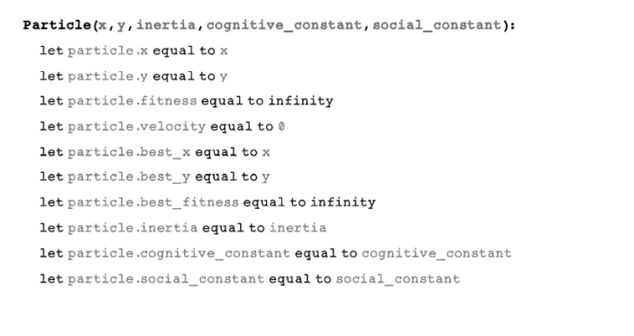
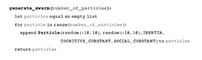
Pseudocode
To fulfill the three attributes of a particle, including position, best position, and velocity, the following properties are required in a constructor of the particle for the various operations of the particle swarm optimization algorithm. Don’t worry about the inertia, cognitive component, and social component right now; they will be explained in upcoming sections:
Particle swarm optimization life cycle
The approach to designing a particle swarm optimization algorithm is based on the problem space being addressed. Each problem has a unique context and a different domain in which data is represented. Solutions to different problems are also measured differently. Let’s dive into how a particle swarm optimization can be designed to solve the drone construction problem.
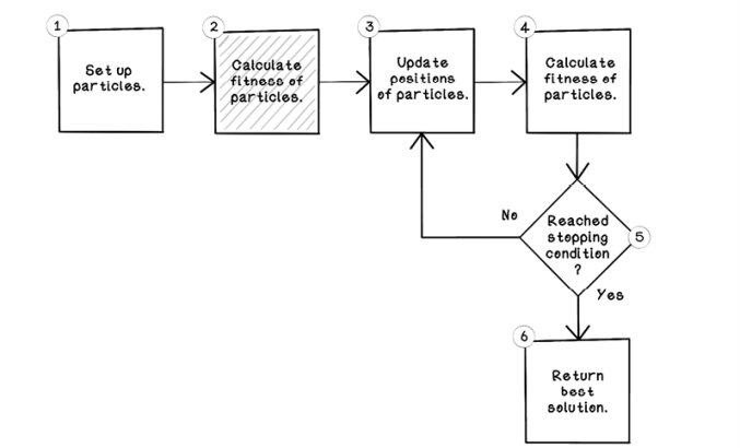
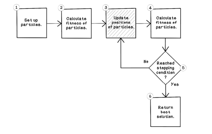
The general life cycle of a particle swarm optimization algorithm is as follows (figure 7.13):
-
Initialize the population of particles. Determine the number of particles to be used, and initialize each particle to a random position in the search space.
-
Calculate the fitness of each particle. Given the position of each particle, determine the fitness of that particle at that position.
-
Update the position of each particle. Repetitively update the position of all the particles, using principles of swarm intelligence. Particles will explore the search space and then converge to good solutions.
-
Determine the stopping criteria. Determine when the particles stop updating and the algorithm stops.
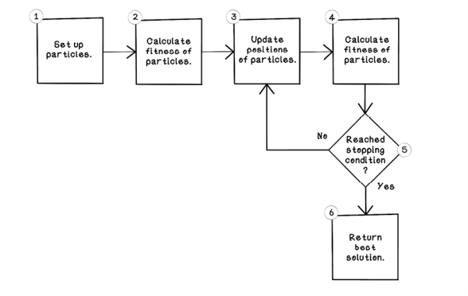
Figure 7.13 The life cycle of a particle swarm optimization algorithm
The particle swarm optimization algorithm is fairly simple, but the details of step 3 are particularly intricate. The following sections look at each step in isolation and uncover the details that make the algorithm work.
Initialize the population of particles
The algorithm starts by creating a specific number of particles, which will remain the same for the lifetime of the algorithm (figure 7.14).
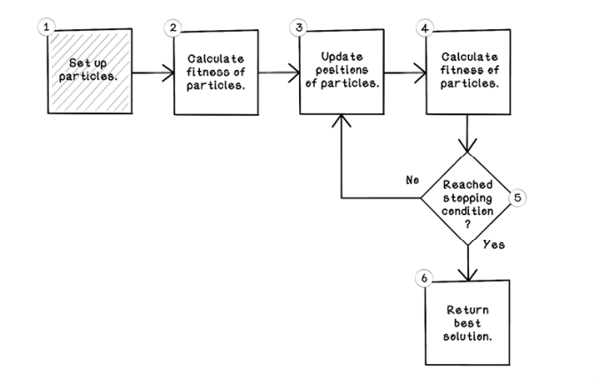
1. Create a swarm of particles with each particle’s position initialized to a random point, and set the particles’ velocities to zero.
Figure 7.14 Set up the particles.
The three factors that are important in initializing the particles are (figure 7.15):
-
Number of particles—The number of particles influences computation. The more particles that exist, the more computation is required. Additionally, more particles will likely mean that converging on a global best solution will take longer because more particles are attracted to their local best solutions. The constraints of the problem also affect the number of particles. A larger search space may need more particles to explore it. There could be as many as 1,000 particles or as few as 4. Usually, 50 to 100 particles produce good solutions without being too computationally expensive.
-
Starting position for each particle—The starting position for each particle should be a random position in all the respective dimensions. It is important that the particles are distributed evenly across the search space. If most of the particles are in a specific region of the search space, they will struggle to find solutions outside that area.
-
Starting velocity for each particle—The velocity of particles is initialized to 0 because the particles have not been affected yet. A good analogy is that birds begin takeoff for flight from a stationary position.

Figure 7.15 A visualization of the initial positions of four particles in a 3D plane
Table 7.2 describes the data encapsulated by each particle at the initialization step of the algorithm. Notice that the velocity is 0; the current fitness and best fitness values are 0 because they have not been calculated yet.
Table 7.2 Data attributes for each particle
|
Particle |
Velocity |
Current aluminum (x) |
Current plastic (y) |
Current fitness |
Best aluminum (x) |
Best plastic (y) |
Best fitness |
|
1 |
0 |
7 |
1 |
0 |
7 |
1 |
0 |
|
2 |
0 |
-1 |
9 |
0 |
-1 |
9 |
0 |
|
3 |
0 |
-10 |
1 |
0 |
-10 |
1 |
0 |
|
4 |
0 |
-2 |
-5 |
0 |
-2 |
-5 |
0 |
Pseudocode
The method to generate a swarm consists of creating an empty list and appending new particles to it. The key factors are:
-
Ensuring that the number of particles is configurable.
-
Ensuring that the random number generation is done uniformly; numbers are distributed across the search space within the constraints. This implementation depends on the features of the random number generator used.
-
Ensuring that the constraints of the search space are specified: in this case, -10 and 10 for both x and y of the particle.
Calculate the fitness of each particle
The next step is calculating the fitness of each particle at its current position. The fitness of particles is calculated every time the entire swarm changes position (figure 7.16).
2. Determine how well each particle solves the problem using the fitness function.
Figure 7.16 Calculate the fitness of the particles.
In the drone scenario, the scientists provided a function in which the result is the amount of drag and wobble given a specific number of aluminum and plastic components. This function is used as the fitness function in the particle swarm optimization algorithm in this example (figure 7.17).

Figure 7.17 The example function for optimizing aluminum (x) and plastic (y)
If x is aluminum and y is plastic, the calculations in figure 7.18 can be made for each particle to determine its fitness by substituting x and y for the values of aluminum and plastic.
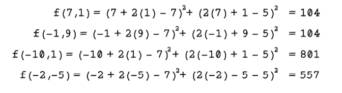
Figure 7.18 Fitness calculations for each particle
Now the table of particles represents the calculated fitness for each particle (table 7.3). It is also set as the best fitness for each particle because it is the only known fitness in the first iteration. After the first iteration, the best fitness for each particle is the best fitness in each specific particle’s history.
Table 7.3 Data attributes for each particle
|
Particle |
Velocity |
Current aluminum (x) |
Current plastic (y) |
Current fitness |
Best aluminum (x) |
Best plastic (y) |
Best fitness |
|
1 |
0 |
7 |
1 |
296 |
7 |
1 |
296 |
|
2 |
0 |
-1 |
9 |
104 |
-1 |
9 |
104 |
|
3 |
0 |
-10 |
1 |
80 |
-10 |
1 |
80 |
|
4 |
0 |
-2 |
-5 |
365 |
-2 |
-5 |
365 |
Exercise: What would the fitness be for the following inputs given the drone fitness function?

|
Particle |
Velocity |
Current aluminum (x) |
Current plastic (y) |
Current fitness |
Best aluminum (x) |
Best plastic (y) |
Best fitness |
|
1 |
0 |
5 |
-3 |
0 |
5 |
-3 |
0 |
|
2 |
0 |
-6 |
-1 |
0 |
-6 |
-1 |
0 |
|
3 |
0 |
7 |
3 |
0 |
7 |
3 |
0 |
|
4 |
0 |
-1 |
9 |
0 |
-1 |
9 |
0 |
Solution: What would the fitness be for the following inputs given the drone fitness function?

Pseudocode
The fitness function is representing the mathematical function in code. Any math library will contain the operations required, such as a power function and a square-root function:

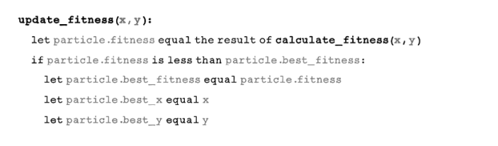
The function for updating the fitness of a particle is also trivial, in that it determines whether the new fitness is better than a past best and then stores that information:
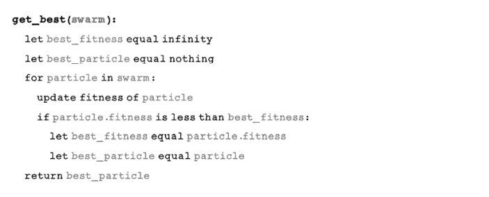
The function to determine the best particle in the swarm iterates through all particles, updates their fitness based on their new positions, and finds the particle that yields the smallest value for the fitness function. In this case, we are minimizing, so a smaller value is better:
Update the position of each particle
The update step of the algorithm is the most intricate, because it is where the magic happens. The update step encompasses the properties of swarm intelligence in nature into a mathematical model that allows the search space to be explored while honing in on good solutions (figure 7.19).
3. Update the velocity and position of all particles while balancing exploration and exploitation of solutions.
Figure 7.19 Update the positions of the particles.
Particles in the swarm update their position given a cognitive ability and factors in the environment around them, such as inertia and what the swarm is doing. These factors influence the velocity and position of each particle. The first step is understanding how velocity is updated. The velocity determines the direction and speed of movement of the particle.
The particles in the swarm move to different points in the search space to find better solutions. Each particle relies on its memory of a good solution and the knowledge of the swarm’s best solution. Figure 7.20 illustrates the movement of the particles in the swarm as their positions are updated.
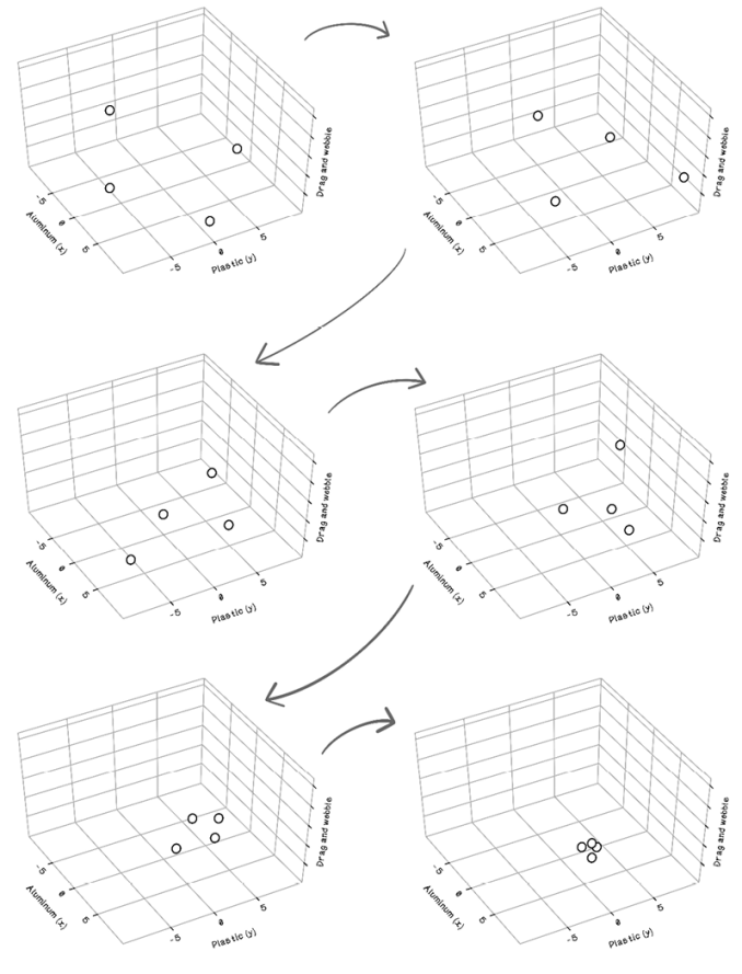
Figure 7.20 The movement of particles over five iterations
The components of updating velocity
Three components are used to calculate the new velocity of each particle: inertia, cognitive, and social. Each component influences the movement of the particle. We will look at each of the components in isolation before diving into how they are combined to update the velocity and, ultimately, the position of a particle:
-
Inertia—The inertia component represents the resistance to movement or change in direction for a specific particle that influences its velocity. The inertia component consists of two values: the inertia magnitude and the current velocity of the particle. The inertia value is a number between 0 and 1.

- A value closer to 0 translates to exploration, potentially taking more iterations.
- A value closer to 1 translates to more exploration for particles in fewer iterations.
-
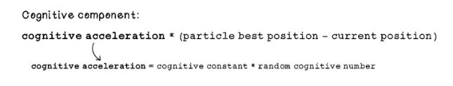
Cognitive—The cognitive component represents the internal cognitive ability of a specific particle. The cognitive ability is a sense of a particle knowing its best position and using that position to influence its movement. The cognitive constant is a number greater than 0 and less than 2. A greater cognitive constant means more exploitation by the particles.
-
Social—The social component represents the ability of a particle to interact with the swarm. A particle knows the best position in the swarm and uses this information to influence its movement. Social acceleration is determined by using a constant and scaling it with a random number. The social constant remains the same for the lifetime of the algorithm, and the random factor encourages diversity in favoring the social factor.
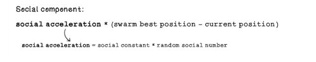
The greater the social constant, the more exploration there will be, because the particle favors its social component more. The social constant is a number between 0 and 2. A greater social constant means more exploration.
Updating velocity
Now that we understand the inertia component, cognitive component, and social component, let’s look at how they can be combined to update a new velocity for the particles (figure 7.21).
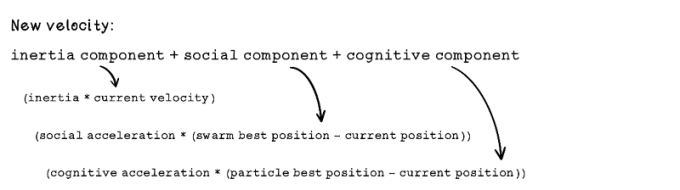
Figure 7.21 Formula to calculate velocity
By looking at the math, we may find it difficult to understand how the different components in the function affect the velocity of the particles. Figure 7.22 depicts how the different factors influence a particle.

Figure 7.22 The intuition of the factors influencing velocity updates
Table 7.4 shows the attributes of each particle after the fitness of each is calculated.
Table 7.4 Data attributes for each particle
|
Particle |
Velocity |
Current aluminum |
Current plastic |
Current fitness |
Best aluminum |
Best plastic |
Best fitness |
|
1 |
0 |
7 |
1 |
296 |
2 |
4 |
296 |
|
2 |
0 |
-1 |
9 |
104 |
-1 |
9 |
104 |
|
3 |
0 |
-10 |
1 |
80 |
-10 |
1 |
80 |
|
4 |
0 |
-2 |
-5 |
365 |
-2 |
-5 |
365 |
Next, we will dive into the velocity update calculations for a particle, given the formulas that we have worked through.
Here are the constant configurations that have been set for this scenario:
-
Inertia is set to 0.2. This setting favors slower exploration.
-
Cognitive constant is set to 0.35. Because this constant is less than the social constant, the social component is favored over an individual particle’s cognitive component.
-
Social constant is set to 0.45. Because this constant is more than the cognitive constant, the social component is favored. Particles put more weight on the best values found by the swarm.
Figure 7.23 describes the calculations of the inertia component, cognitive component, and social component for the velocity update formula.
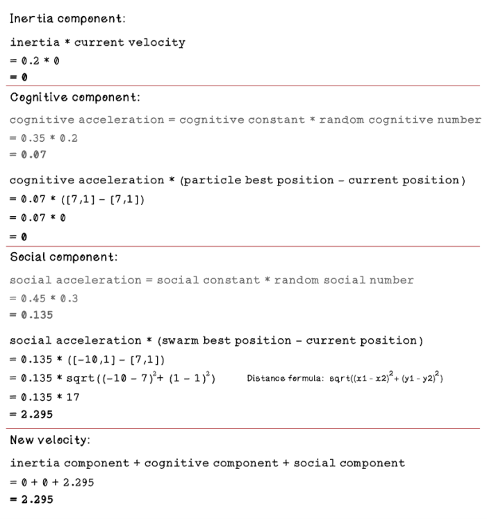
Figure 7.23 Particle velocity calculation walkthrough
After these calculations have been completed for all particles, the velocity of each particle is updated, as represented in table 7.5.
Table 7.5 Data attributes for each particle
|
Particle |
Velocity |
Current aluminum |
Current plastic |
Current fitness |
Best aluminum |
Best plastic |
Best fitness |
|
1 |
2.295 |
7 |
1 |
296 |
7 |
1 |
296 |
|
2 |
1.626 |
-1 |
9 |
104 |
-1 |
9 |
104 |
|
3 |
2.043 |
-10 |
1 |
80 |
-10 |
1 |
80 |
|
4 |
1.35 |
-2 |
-5 |
365 |
-2 |
-5 |
365 |
Position update
Now that we understand how velocity is updated, we can update the current position of each particle, using the new velocity (figure 7.24).

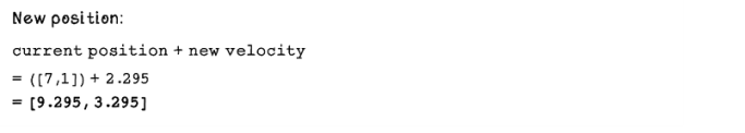
Figure 7.24 Calculating the new position of a particle
By adding the current position and new velocity, we can determine the new position of each particle and update the table of particle attributes with the new velocities. Then the fitness of each particle is calculated again, given its new position, and its best position is remembered (table 7.6).
Table 7.6 Data attributes for each particle
|
Particle |
Velocity |
Current aluminum |
Current plastic |
Current fitness |
Best aluminum |
Best plastic |
Best fitness |
|
1 |
2.295 |
9.925 |
3.325 |
721.286 |
7 |
1 |
296 |
|
2 |
1.626 |
0.626 |
10 |
73.538 |
0.626 |
10 |
73.538 |
|
3 |
2.043 |
7.043 |
1.043 |
302.214 |
-10 |
1 |
80 |
|
4 |
1.35 |
-0.65 |
-3.65 |
179.105 |
-0.65 |
-3.65 |
179.105 |
Calculating the initial velocity for each particle in the first iteration is fairly simple because there was no previous best position for each particle—only a swarm best position that affected only the social component.
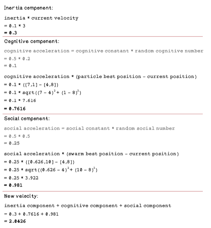
Let’s examine what the velocity update calculation will look like with the new information for each particle’s best position and the swarm’s new best position. Figure 7.25 describes the calculation for particle 1 in the list.
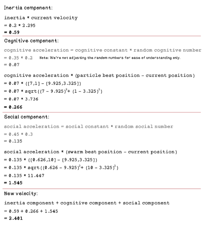
Figure 7.25 Particle velocity calculation walkthrough
In this scenario, the cognitive component and the social component both play a role in updating the velocity, whereas the scenario described in figure 7.23 is influenced by the social component, due to it being the first iteration.
Particles move to different positions over several iterations. Figure 7.26 depicts the particles’ movement and their convergence on a solution.
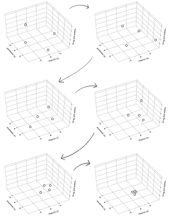
Figure 7.26 A visualization of the movement of particles in the search space
In the last frame of figure 7.26, all the particles have converged in a specific region in the search space. The best solution from the swarm will be used as the final solution. In real-world optimization problems, it is not possible to visualize the entire search space (which would make optimization algorithms unnecessary). But the function that we used for the drone example is a known function called the Booth function. By mapping it to the 3D Cartesian plane, we can see that the particles indeed converge on the minimum point in the search space (figure 7.27).

Figure 7.27 Visualization of convergence of particles and a known surface
After using the particle swarm optimization algorithm for the drone example, we find that the optimal ratio of aluminum and plastic to minimize drag and wobble is 1:3—that is, 1 part aluminum and 3 parts plastic. When we feed these values into the fitness function, the result is 0, which is the minimum value for the function.
Pseudocode
The update step can seem to be daunting, but if the components are broken into simple focused functions, the code becomes simpler and easier to write, use, and understand. The first functions are the inertia calculation function, the cognitive acceleration function, and the social acceleration function. We also need a function to measure the distance between two points, which is represented by squaring the sum of the square of the difference in x values summed with the square of the difference in the y values:
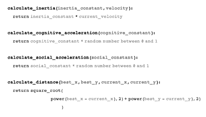
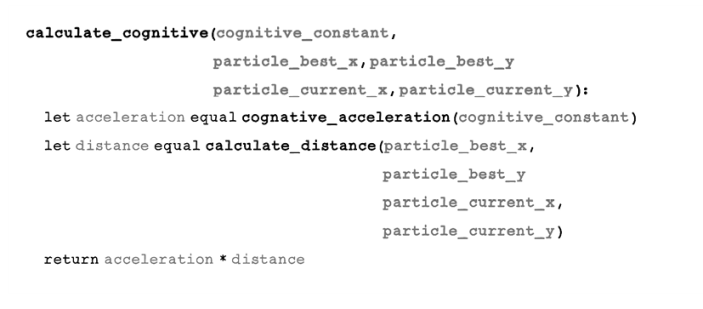
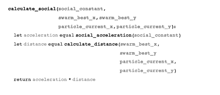
The cognitive component is calculated by finding the cognitive acceleration, using the function that we defined in an earlier section, and the distance between the particle’s best position and its current position:
The social component is calculated by finding the social acceleration, using the function that we defined earlier, and the distance between the swarm’s best position and the particle’s current position:
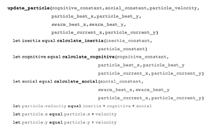
The update function wraps everything that we have defined to carry out the actual update of a particle’s velocity and position. The velocity is calculated by using the inertia component, cognitive component, and social component. The position is calculated by adding the new velocity to the particle’s current position:
Exercise: Calculate the new velocity and position for particle 1 given the following information about the particles
-
Inertia is set to 0.1.
-
The cognitive constant is set to 0.5, and the cognitive random number is 0.2.
- The social constant is set to 0.5, and the cognitive random number is 0.5.
Particle
Velocity
Current aluminum
Current plastic
Current fitness
Best aluminum
Best plastic
Best fitness
1
3
4
8
721.286
7
1
296
2
4
3
3
73.538
0.626
10
73.538
3
1
6
2
302.214
-10
1
80
4
2
2
5
179.105
-0.65
-3.65
179.105
Solution: Calculate the new velocity and position for particle 1 given the following information about the particles
Determine the stopping criteria
The particles in the swarm cannot keep updating and searching indefinitely. A stopping criterion needs to be determined to allow the algorithm to run for a reasonable number of iterations to find a suitable solution (figure 7.28).

5. Determine how many iterations the algorithm runs for—this is the number of times all particles are updated.
Figure 7.28 Has the algorithm reached a stopping condition?
The number of iterations influences several aspects of finding solutions, including:
-
Exploration—Particles require time to explore the search space to find areas with better solutions. Exploration is also influenced by the constants defined in the update velocity function.
-
Exploitation—Particles should converge on a good solution after reasonable exploration occurs.
A strategy to stop the algorithm is to examine the best solution in the swarm and determine whether it is stagnating. Stagnation occurs when the value of the best solution doesn’t change or doesn’t change by a significant amount. Running more iterations in this scenario will not help find better solutions. When the best solution stagnates, the parameters in the update function can be adjusted to favor more exploration. If more exploration is desired, this adjustment usually means more iterations. Stagnation could mean that a good solution was found or that that the swarm is stuck on a local best solution. If enough exploration occurred at the start, and the swarm gradually stagnates, the swarm has converged on a good solution (figure 7.29).

Figure 7.29 Exploration converging and exploiting
Use cases for particle swarm optimization algorithms
Particle swarm optimization algorithms are interesting because they simulate a natural phenomenon, which makes them easier to understand, but they can be applied to a range of problems at different levels of abstraction. This chapter looked at an optimization problem for drone manufacturing, but particle swarm optimization algorithms can be used in conjunction with other algorithms, such as artificial neural networks, playing a small but critical role in finding good solutions.
One interesting application of a particle swarm optimization algorithm is deep brain stimulation. The concept involves installing probes with electrodes into the human brain to stimulate it to treat conditions such as Parkinson’s disease. Each probe contains electrodes that can be configured in different directions to treat the condition correctly per patient. Researchers at the University of Minnesota have developed a particle swarm optimization algorithm to optimize the direction of each electrode to maximize the region of interest, minimize the region of avoidance, and minimize energy use. Because particles are effective in searching these multidimensional problem spaces, the particle swarm optimization algorithm is effective for finding optimal configurations for electrodes on the probes (figure 7.30).
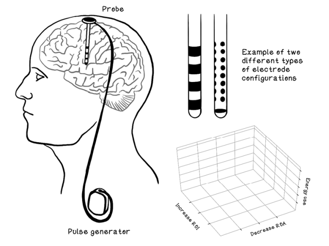
Figure 7.30 Example of factors involved for probes in deep brain stimulation
Here are some other real-world applications of particle swarm optimization algorithms:
-
Optimizing weights in an artificial neural network—Artificial neural networks are modeled on an idea of how the human brain works. Neurons pass signals to other neurons, and each neuron adjusts the signal before passing it on. An artificial neural network uses weights to adjust each signal. The power of the network is finding the right balance of weights to form patterns in relationships of the data. Adjusting weights is computationally expensive, as the search space is massive. Imagine having to brute-force every possible decimal number combination for 10 weights. That process would take years.
Don’t panic if this concept sounds confusing. We explore how artificial neural networks operate in chapter 9. Particle swarm optimization can be used to adjust the weights of neural networks faster, because it seeks optimal values in the search space without exhaustively attempting each one.
-
Motion tracking in videos—Motion tracking of people is a challenging task in computer vision. The goal is to identify the poses of people and imply a motion by using the information from the images in the video alone. People move differently, even though their joints move similarly. Because the images contain many aspects, the search space becomes large, with many dimensions to predict the motion for a person. Particle swarm optimization works well in high-dimension search spaces and can be used to improve the performance of motion tracking and prediction.
-
Speech enhancement in audio—Audio recordings are nuanced. There is always background noise that may interfere with what someone is saying in the recording. A solution is to remove the noise from recorded speech audio clips. A technique used for this purpose is filtering the audio clip with noise and comparing similar sounds to remove the noise in the audio clip. This solution is still complex, as reduction of certain frequencies may be good for parts of the audio clip but may deteriorate other parts of it. Fine searching and matching must be done for good noise removal. Traditional methods are slow, as the search space is large. Particle swarm optimization works well in large search spaces and can be used to speed the process of removing noise from audio clips.
Summary of particle swarm optimization