This chapter covers

• The intuition of planning and searching

• Identifying problems suited to be solved using search algorithms

• Representing problem spaces in a way suitable to be processed by search algorithms

• Understanding and designing fundamental search algorithms to solve problems

What are planning and searching?

When we think about what makes us intelligent, the ability to plan before carrying out actions is a prominent attribute. Before embarking on a trip to a different country, before starting a new project, before writing functions in code, planning happens. Planning happens at different levels of detail in different contexts to strive for the best possible outcome when carrying out the tasks involved in accomplishing goals (figure 2.1).

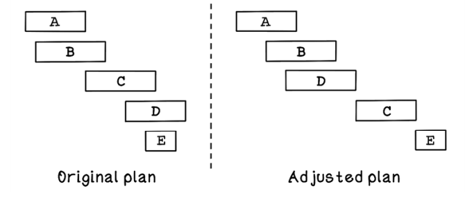
Figure 2.1 Example of how plans change in projects

Plans rarely work out perfectly in the way we envision at the start of an endeavor. We live in a world in which environments are constantly changing, so it is impossible to account for all the variables and unknowns along the way. Regardless of the plan we started with, we almost always deviate due to changes in the problem space. We need to (again) make a new plan from our current point going forward, if after we take more steps, unexpected events occur that require another iteration of planning to meet the goals. As a result, the final plan that is carried out is usually different from the original one.

Searching is a way to guide planning by creating steps in a plan. When we plan a trip, for example, we search for routes to take, evaluate the stops along the way and what they offer, and search for accommodations and activities that align with our liking and budget. Depending on the results of these searches, the plan changes.

Suppose that we have settled on a trip to the beach, which is 500 kilometers away, with two stops: one at a petting zoo and one at a pizza restaurant. We will sleep at a lodge close to the beach on arrival and partake in three activities. The trip to the destination will take approximately 8 hours. We’re also taking a shortcut private road after the restaurant, but it’s open only until 2:00.

We start the trip, and everything is going according to plan. We stop at the petting zoo and see some wonderful animals. We drive on and start getting hungry; it’s time for the stop at the restaurant. But to our surprise, the restaurant recently went out of business. We need to adjust our plan and find another place to eat, which involves searching for a close-by establishment of our liking and adjusting our plan.

After driving around for a while, we find a restaurant, enjoy a pizza, and get back on the road. Upon approaching the shortcut private road, we realize that it’s 2:20. The road is closed; yet again, we need to adjust our plan. We search for a detour and find that it will add 120 kilometers to our drive, and we will need to find accommodations for the night at a different lodge before we even get to the beach. We search for a place to sleep and plot out our new route. Due to lost time, we can partake in only two activities at the destination. The plan has been adjusted heavily through searching for different options that satisfy each new situation, but we end up having a great adventure en route to the beach.

This example shows how search is used for planning and influences planning toward desirable outcomes. As the environment changes, our goals may change slightly, and our path to them inevitably needs to be adjusted (figure 2.2). Adjustments in plans can almost never be anticipated and need to be made as required.

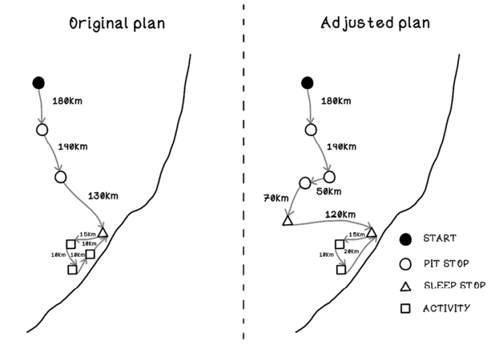
Figure 2.2 Original plan versus adjusted plan for a road trip

Searching involves evaluating future states toward a goal with the aim of finding an optimal path of states until the goal is reached. This chapter centers on different approaches to searching depending on different types of problems. Searching is an old but powerful tool for developing intelligent algorithms to solve problems.

Cost of computation: The reason for smart algorithms

In programming, functions consist of operations, and due to the way that traditional computers work, different functions use different amounts of processing time. The more computation required, the more expensive the function is. Big O notation is used to describe the complexity of a function or algorithm. Big O notation models the number of operations required as the input size increases. Here are some examples and associated complexities:

• A single operation that prints Hello World—This operation is a single operation, so the cost of computation is O(1).

• A function that iterates over a list and prints each item in the list—The number of operations is dependent on the number of items in the list. The cost is O(n).

• A function that compares every item in a list with every item in another list—This operation costs O(n²).

Figure 2.3 depicts different costs of algorithms. Algorithms that require operations to explore as the size of the input increases are the worst-performing; algorithms that require a more constant number of operations as the number of inputs increases are better.

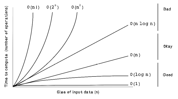
Figure 2.3 Big O complexity

Understanding that different algorithms have different computation costs is important because addressing this is the entire purpose of intelligent algorithms that solve problems well and quickly. Theoretically, we can solve almost any problem by brute-forcing every possible option until we find the best one, but in reality, the computation could take hours or even years, which makes it infeasible for real-world scenarios.

Problems applicable to searching algorithms

Almost any problem that requires a series of decisions to be made can be solved with search algorithms. Depending on the problem and the size of the search space, different algorithms may be employed to help solve it. Depending on the search algorithm selected and the configuration used, the optimal solution or a best available solution may be found. In other words, a good solution will be found, but it might not necessarily be the best solution. When we speak about a “good solution” or “optimal solution,” we are referring to the performance of the solution in addressing the problem at hand.

One scenario in which search algorithms are useful is being stuck in a maze and attempting to find the shortest path to a goal. Suppose that we’re in a square maze consisting of an area of 10 blocks by 10 blocks (figure 2.4). There exists a goal that we want to reach and barriers that we cannot step into. The objective is to find a path to the goal while avoiding barriers with as few steps as possible by moving north, south, east, or west. In this example, the player cannot move diagonally.

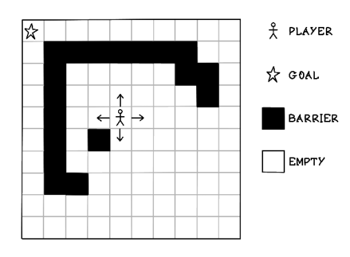
Figure 2.4 An example of the maze problem

How can we find the shortest path to the goal while avoiding barriers? By evaluating the problem as a human, we can try each possibility and count the moves. Using trial and error, we can find the paths that are the shortest, given that this maze is relatively small.

Using the example maze, figure 2.5 depicts some possible paths to reach the goal, although note that we don’t reach the goal in option 1.

Figure 2.5 Examples of possible paths to the maze problem

By looking at the maze and counting blocks in different directions, we can find several solutions to the problem. Five attempts have been made to find four successful solutions out of an unknown number of solutions. It will take exhaustive effort to attempt to compute all possible solutions by hand:

• Attempt 1 is not a valid solution. It took 4 actions, and the goal was not found.

• Attempt 2 is a valid solution, taking 17 actions to find the goal.

• Attempt 3 is a valid solution, taking 23 actions to find the goal.

• Attempt 4 is a valid solution, taking 17 actions to find the goal.

• Attempt 5 is the best valid solution, taking 15 actions to find the goal. Although this attempt is the best one, it was found by chance.

If the maze were a lot larger, like the one in figure 2.6, it would take an immense amount of time to compute the best possible path manually. Search algorithms can help.

Figure 2.6 A large example of the maze problem

Our power as humans is to perceive a problem visually, understand it, and find solutions given the parameters. As humans, we understand and interpret data and information in an abstract way. A computer cannot yet understand generalized information in the natural form that we do. The problem space needs to be represented in a form that is applicable to computation and can be processed with search algorithms.

Representing state: Creating a framework to represent problem spaces and solutions

When representing data and information in a way that a computer can understand, we need to encode it logically so that it can be understood objectively. Although the data will be encoded subjectively by the person who performs the task, there should be a concise, consistent way to represent it.

Let’s clarify the difference between data and information. Data is raw facts about something, and information is an interpretation of those facts that provides insight about the data in the specific domain. Information requires context and processing of data to provide meaning. As an example, each individual distance traveled in the maze example is data, and the sum of the total distance traveled is information. Depending on the perspective, level of detail, and desired outcome, classifying something as data or information can be subjective to the context and person or team (figure 2.7).

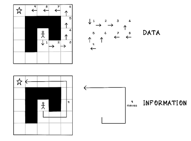
Figure 2.7 Data versus information

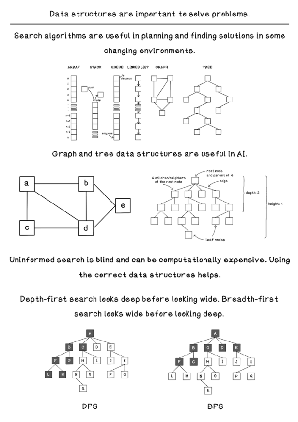
Data structures are concepts in computer science used to represent data in a way that is suitable for efficient processing by algorithms. A data structure is an abstract data type consisting of data and operations organized in a specific way. The data structure we use is influenced by the context of the problem and the desired goal.

An example of a data structure is an array, which is simply a collection of data. Different types of arrays have different properties that make them efficient for different purposes. Depending on the programming language used, an array could allow each value to be of a different type or require each value to be the same type, or the array may disallow duplicate values. These different types of arrays usually have different names. The features and constraints of different data structures also enable more efficient computation (figure 2.8).

Figure 2.8 Data structures used with algorithms

Other data structures are useful in planning and searching. Trees and graphs are ideal for representing data in a way that search algorithms can use.

Graphs: Representing search problems and solutions

A graph is a data structure containing several states with connections among them. Each state in a graph is called a node (or sometimes a vertex), and a connection between two states is called an edge. Graphs are derived from graph theory in mathematics and used to model relationships among objects. Graphs are useful data structures that are easy for humans to understand, due to the ease of representing them visually as well as to their strong logical nature, which is ideal for processing via various algorithms (figure 2.9).

Figure 2.9 The notation used to represent graphs

Figure 2.10 is a graph of the trip to the beach discussed in the first section of this chapter. Each stop is a node on the graph; each edge between nodes represent points traveled between; and the weights on each edge indicate the distance traveled.

Figure 2.10 The example road trip represented as a graph

Representing a graph as a concrete data structure

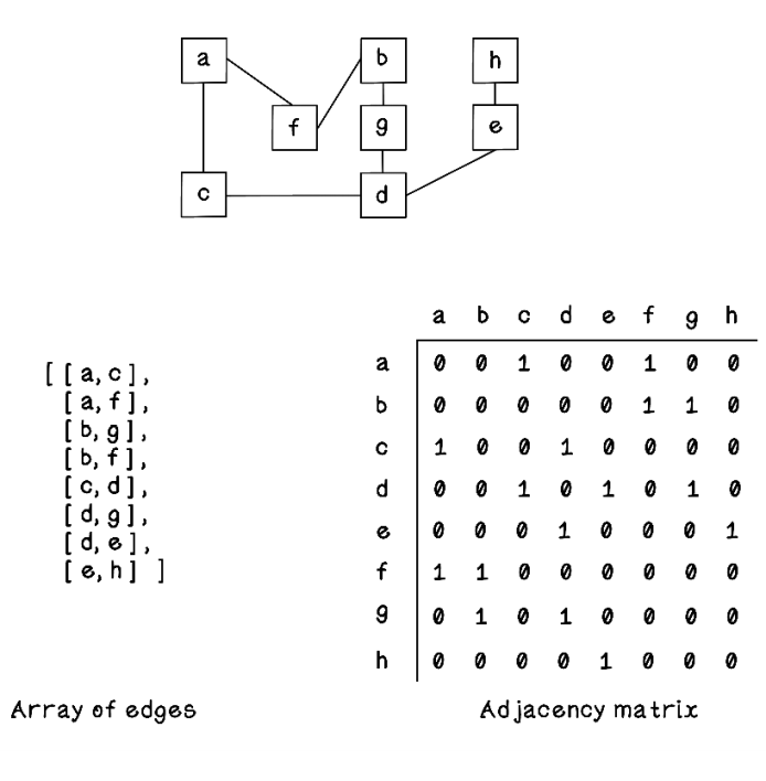
A graph can be represented in several ways for efficient processing by algorithms. At its core, a graph can be represented by an array of arrays that indicates relationships among nodes, as shown in figure 2.11. It is sometimes useful to have another array that simply lists all nodes in the graph so that the distinct nodes do not need to be inferred from the relationships.

Figure 2.11 Representing a graph as an array of arrays

Other representations of graphs include an incidence matrix, an adjacency matrix, and an adjacency list. By looking at the names of these representations, you see that the adjacency of nodes in a graph is important. An adjacent node is a node that is connected directly to another node.

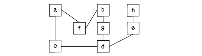
Exercise: Represent a Graph as a Matrix

How would you represent the following graph using edge arrays?

Solution: Represent a Graph as a Matrix

Trees: The concrete structures used to represent search solutions

A tree is a popular data structure that simulates a hierarchy of values or objects. A hierarchy is an arrangement of things in which a single object is related to several other objects below it. A tree is a connected acyclic graph—every node has an edge to another node, and no cycles exist.

In a tree, the value or object represented at a specific point is called a node. Trees typically have a single root node with zero or more child nodes that could contain subtrees. Let’s take a deep breath and jump into some terminology. When a node has connected nodes, the root node is called the parent. You can apply this thinking recursively. A child node may have its own child nodes, which may also contain subtrees. Each child node has a single parent node. A node without any children is a leaf node.

Trees also have a total height. The level of specific nodes is called a depth.

The terminology used to relate family members is heavily used in working with trees. Keep this analogy in mind, as it will help you connect the concepts in the tree data structure. Note that in figure 2.12, the height and depth are indexed from 0 from the root node.

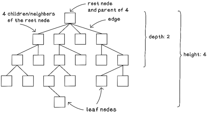
Figure 2.12 The main attributes of a tree

The topmost node in a tree is called the root node. A node directly connected to one or more other nodes is called a parent node. The nodes connected to a parent node are called child nodes or neighbors. Nodes connected to the same parent node are called siblings. A connection between two nodes is called an edge.

A path is a sequence of nodes and edges connecting nodes that are not directly connected. A node connected to another node by following a path away from the root node is called a descendent, and a node connected to another node by following a path toward the root node is called an ancestor. A node with no children is called a leaf node. The term degree is used to describe the number of children a node has; therefore, a leaf node has degree zero.

Figure 2.13 represents a path from the start point to the goal for the maze problem. This path contains nine nodes that represent different moves being made in the maze.

Figure 2.13 A solution to the maze problem represented as a tree

Trees are the fundamental data structure for search algorithms, which we will be diving into next. Sorting algorithms are also useful in solving certain problems and computing solutions more efficiently. If you’re interested in learning more about sorting algorithms, take a look at Grokking Algorithms (Manning Publications).

Uninformed search: Looking blindly for solutions

Uninformed search is also known as unguided search, blind search, or brute-force search. Uninformed search algorithms have no additional information about the domain of the problem apart from the representation of the problem, which is usually a tree.

Think about exploring things you want to learn. Some people might look at a wide breadth of different topics and learn the basics of each, whereas other people might choose one narrow topic and explore its subtopics in depth. This is what breadth-first search (BFS) and depth-first search (DFS) involve, respectively. Depth-first search explores a specific path from the start until it finds a goal at the utmost depth. Breadth-first search explores all options at a specific depth before moving to options deeper in the tree.

Consider the maze scenario (figure 2.14). In attempting to find an optimal path to the goal, assume the following simple constraint to prevent getting stuck in an endless loop and prevent cycles in our tree: the player cannot move into a block that they have previously occupied. Because uninformed algorithms attempt every possible option at every node, creating a cycle will cause the algorithm to fail catastrophically.

Figure 2.14 The constraint for the maze problem

This constraint prevents cycles in the path to the goal in our scenario. But this constraint will introduce problems if, in a different maze with different constraints or rules, moving into a previously occupied block more than once is required for the optimal solution.

In figure 2.15, all possible paths in the tree are represented to highlight the different options available. This tree contains seven paths that lead to the goal and one path that results in an invalid solution, given the constraint of not moving to previously occupied blocks. It’s important to understand that in this small maze, representing all the possibilities is feasible. The entire point of search algorithms, however, is to search or generate these trees iteratively, because generating the entire tree of possibilities up front is inefficient due to being computationally expensive.

It is also important to note that the term visiting is used to indicate different things. The player visits blocks in the maze. The algorithm also visits nodes in the tree. The order of choices will influence the order of nodes being visited in the tree. In the maze example, the priority order of movement is north, south, east, and then west.

Figure 2.15 All possible movement options represented as a tree

Now that we understand the ideas behind trees and the maze example, let’s explore how search algorithms can generate trees that seek out paths to the goal.

Breadth-first search: Looking wide before looking deep

Breadth-first search is an algorithm used to traverse or generate a tree. This algorithm starts at a specific node, called the root, and explores every node at that depth before exploring the next depth of nodes. It essentially visits all children of nodes at a specific depth before visiting the next depth of child until it finds a goal leaf node.

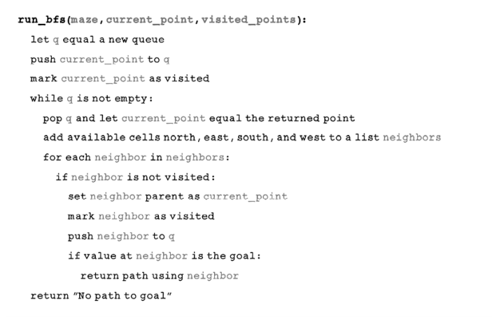
The breadth-first search algorithm is best implemented by using a first-in, first-out queue in which the current depths of nodes are processed, and their children are queued to be processed later. This order of processing is exactly what we require when implementing this algorithm.

Figure 2.16 is a flow chart describing the sequence of steps involved in the breadth-first search algorithm.

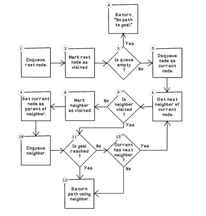
Figure 2.16 Flow of the breadth-first search algorithm

Here are some notes and additional remarks about each step in the process:

1. Enqueue root node. The breadth-first search algorithm is best implemented with a queue. Objects are processed in the sequence in which they are added to the queue. This process is also known as first in, first out (FIFO). The first step is adding the root node to the queue. This node will represent the starting position of the player on the map.

2. Mark root node as visited. Now that the root node has been added to the queue for processing, it is marked as visited to prevent it from being revisited for no reason.

3. Is queue empty? If the queue is empty (all nodes have been processed after many iterations), and if no path has been returned in step 12 of the algorithm, there is no path to the goal. If there are still nodes in the queue, the algorithm can continue its search to find the goal.

4. Return No path to goal. This message is the one possible exit from the algorithm if no path to the goal exists.

5. Dequeue node as current node. By pulling the next object from the queue and setting it as the current node of interest, we can explore its possibilities. When the algorithm starts, the current node will be the root node.

6. Get next neighbor of current node. This step involves getting the next possible move in the maze from the current position by referencing the maze and determining whether a north, south, east, or west movement is possible.

7. Is neighbor visited? If the current neighbor has not been visited, it hasn’t been explored yet and can be processed now.

8. Mark neighbor as visited. This step indicates that this neighbor node has been visited.

9. Set current node as parent of neighbor. Set the origin node as the parent of the current neighbor. This step is important for tracing the path from the current neighbor to the root node. From a map perspective, the origin is the position that the player moved from, and the current neighbor is the position that the player moved to.

10. Enqueue neighbor. The neighbor node is queued for its children to be explored later. This queuing mechanism allows nodes from each depth to be processed in that order.

11. Is goal reached? This step determines whether the current neighbor contains the goal that the algorithm is searching for.

12. Return path using neighbor. By referencing the parent of the neighbor node, then the parent of that node, and so on, the path from the goal to the root will be described. The root node will be a node without a parent.

13. Current has next neighbor? If the current node has more possible moves to make in the maze, jump to step 6 for that move.

Let’s walk through what that would look like in a simple tree. Notice that as the tree is explored and nodes are added to the FIFO queue, the nodes are processed in the order desired by leveraging the queue (figures 2.17 and 2.18).

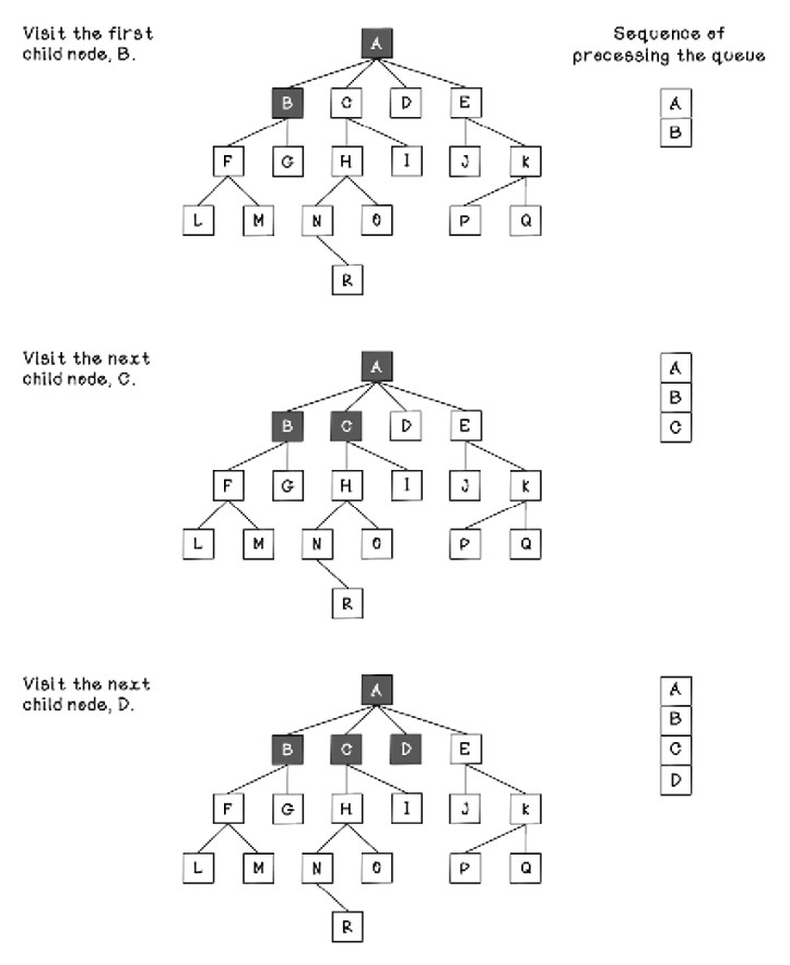
Figure 2.17 The sequence of tree processing using breadth-first search (part 1)

Figure 2.18 The sequence of tree processing using breadth-first search ( part 2)

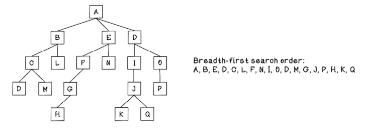
Exercise: Determine the path to the solution

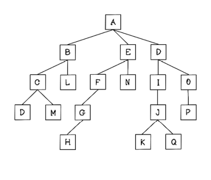
What would be the order of visits using breadth-first search for the following tree?

Solution: Determine the path to the solution

In the maze example, the algorithm needs to understand the current position of the player in the maze, evaluate all possible choices for movement, and repeat that logic for each choice of movement made until the goal is reached. By doing this, the algorithm generates a tree with a single path to the goal.

It is important to understand that the processes of visiting nodes in a tree is used to generate nodes in a tree. We are simply finding related nodes through a mechanism.

Each path to the goal consists of a series of moves to reach the goal. The number of moves in the path is the distance to reach the goal for that path, which we will call the cost. The number of moves also equals the number of nodes visited in the path, from the root node to the leaf node that contains the goal. The algorithm moves down the tree depth by depth until it finds a goal; then it returns the first path that got it to the goal as the solution. There may be a more optimal path to the goal, but because breadth-first search is uninformed, it is not guaranteed to find that path.

NOTE In the maze example, all search algorithms used terminate when they’ve found a solution to the goal. It is possible to allow these algorithms to find multiple solutions with a small tweak to each algorithm, but the best use cases for search algorithms find a single goal, as it is often too expensive to explore the entire tree of possibilities.

Figure 2.19 shows the generation of a tree using movements in the maze. Because the tree is generated using breadth-first search, each depth is generated to completion before looking at the next depth (figure 2.20).

Figure 2.19 Maze movement tree generation using breadth-first search

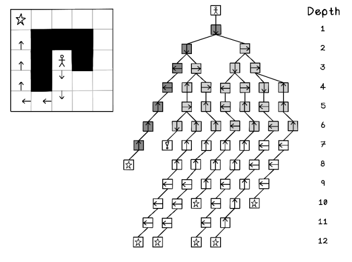
Figure 2.20 Nodes visited in the entire tree after breadth-first search

Pseudocode

As mentioned previously, the breadth-first search algorithm uses a queue to generate a tree one depth at a time. Having a structure to store visited nodes is critical to prevent getting stuck in cyclic loops; and setting the parent of each node is important for determining a path from the starting point in the maze to the goal:

Depth-first search: Looking deep before looking wide

Depth-first search is another algorithm used to traverse a tree or generate nodes and paths in a tree. This algorithm starts at a specific node and explores paths of connected nodes of the first child, doing this recursively until it reaches the farthest leaf node before backtracking and exploring other paths to leaf nodes via other child nodes that have been visited. Figure 2.21 illustrates the general flow of the depth-first search algorithm.

Figure 2.21 Flow of the depth-first search algorithm

Let’s walk through the flow of the depth-first search algorithm:

1. Add root node to stack. The depth-first search algorithm can be implemented by using a stack in which the last object added is processed first. This process is known as last in, first out (LIFO). The first step is adding the root node to the stack.

2. Is stack empty? If the stack is empty and no path has been returned in step 8 of the algorithm, there is no path to the goal. If there are still nodes in the stack, the algorithm can continue its search to find the goal.

3. Return No path to goal. This return is the one possible exit from the algorithm if no path to the goal exists.

4. Pop node from stack as current node. By pulling the next object from the stack and setting it as the current node of interest, we can explore its possibilities.

5. Is current node visited? If the current node has not been visited, it hasn’t been explored yet and can be processed now.

6. Mark current node as visited. This step indicates that this node has been visited to prevent unnecessary repeat processing of it.

7. Is goal reached? This step determines whether the current neighbor contains the goal that the algorithm is searching for.

8. Return path using current node. By referencing the parent of the current node, then the parent of that node, and so on, the path from the goal to the root is described. The root node will be a node without a parent.

9. Current has next neighbor? If the current node has more possible moves to make in the maze, that move can be added to the stack to be processed. Otherwise, the algorithm can jump to step 2, where the next object in the stack can be processed if the stack is not empty. The nature of the LIFO stack allows the algorithm to process all nodes to a leaf node depth before backtracking to visit other children of the root node.

10. Set current node as parent of neighbor. Set the origin node as the parent of the current neighbor. This step is important for tracing the path from the current neighbor to the root node. From a map perspective, the origin is the position that the player moved from, and the current neighbor is the position that the player moved to.

11. Add neighbor to stack. The neighbor node is added to the stack for its children to be explored later. Again, this stacking mechanism allows nodes to be processed to the utmost depth before processing neighbors at shallow depths.

Figures 2.22 and 2.23 explore how the LIFO stack is used to visit nodes in the order desired by depth-first search. Notice that nodes get pushed onto and popped from the stack as the depths of the nodes visited progress. The term push describes adding objects to a stack, and the term pop describes removing the topmost object from the stack.

Figure 2.22 The sequence of tree processing using depth-first search (part 1)

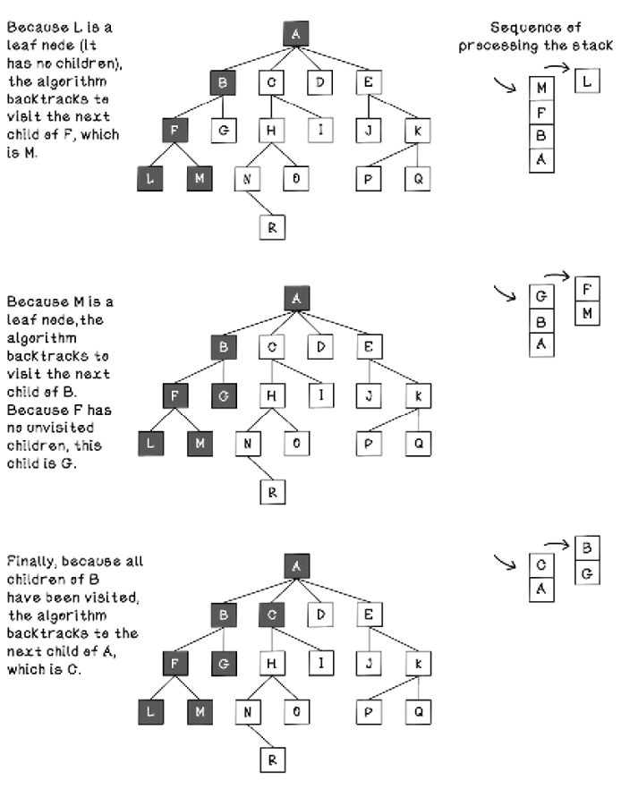
Figure 2.23 The sequence of tree processing using depth-first search (part 2)

Exercise: Determine the path to the solution

What would the order of visits be in depth-first search for the following tree?

Solution: Determine the path to the solution

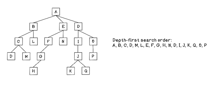
It is important to understand that the order of children matters substantially when using depth-first search, as the algorithm explores the first child until it finds leaf nodes before backtracking.

In the maze example, the order of movement (north, south, east, and west) influences the path to the goal that the algorithm finds. A change in order will result in a different solution. The forks represented in figures 2.24 and 2.25 don’t matter; what matters is the order of the movement choices in our maze example.

Figure 2.24 Maze movement tree generation using depth-first search

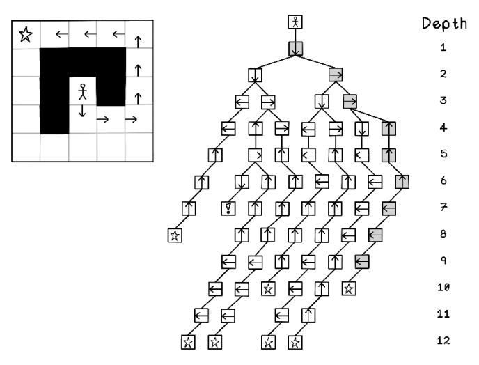
Figure 2.25 Nodes visited in the entire tree after depth-first search

Pseudocode

Although the depth-first search algorithm can be implemented with a recursive function, we’re looking at an implementation that is achieved with a stack to better represent the order in which nodes are visited and processed. It is important to keep track of the visited points so that the same nodes do not get visited unnecessarily, creating cyclic loops:

Use cases for uninformed search algorithms

Uninformed search algorithms are versatile and useful in several real-world use cases, such as

• Finding paths between nodes in a network—When two computers need to communicate over a network, the connection passes through many connected computers and devices. Search algorithms can be used to establish a path in that network between two devices.

• Crawling web pages—Web searches allow us to find information on the internet across a vast number of web pages. To index these web pages, crawlers typically read the information on each page, as well as follow each link on that page recursively. Search algorithms are useful for creating crawlers, metadata structures, and relationships between content.

• Finding social network connections—Social media applications contain many people and their relationships. Bob may be friends with Alice, for example, but not direct friends with John, so Bob and John are indirectly related via Alice. A social media application can suggest that Bob and John should become friends because they may know each other through their mutual friendship with Alice.

Optional: More about graph categories

Graphs are useful for many computer science and mathematical problems, and due to the nature of different types of graphs, different principles and algorithms may apply to specific categories of graphs. A graph is categorized based on its overall structure, number of nodes, number of edges, and interconnectivity between nodes.

These categories of graphs are good to know about, as they are common and sometimes referenced in search and other AI algorithms:

• Undirected graph—No edges are directed. Relationships between two nodes are mutual. As with roads between cities, there are roads traveling in both directions.

• Directed graph—Edges indicate direction. Relationships between two nodes are explicit. As in a graph representing a child of a parent, the child cannot be the parent of its parent.

• Disconnected graph—One or more nodes are not connected by any edges. As in a graph representing physical contact between continents, some nodes are not connected. Like continents, some are connected by land, and others are separated by oceans.

• Acyclic graph—A graph that contains no cycles. As with time as we know it, the graph does not loop back to any point in the past (yet).

• Complete graph—Every node is connected to every other node by an edge. As in the lines of communication in a small team, everyone talks to everyone else to collaborate.

• Complete bipartite graph—A vertex partition is a grouping of vertices. Given a vertex partition, every node from one partition is connected to every node of the other partition with edges. As at a cheese-tasting event, typically, every person tastes every type of cheese.

• Weighted graph—A graph in which the edges between nodes have a weight. As in the distance between cities, some cities are farther than others. The connections “weigh” more.

It is useful to understand the different types of graphs to best describe the problem and use the most efficient algorithm for processing (figure 2.26). Some of these categories of graphs are discussed in upcoming chapters, such as chapter 6 on ant colony optimization and chapter 8 on neural networks.

Figure 2.26 Types of graphs

Optional: More ways to represent graphs

Depending on the context, other encodings of graphs may be more efficient for processing or easier to work with, depending on the programming language and tools you’re using.

Incidence matrix

An incidence matrix uses a matrix in which the height is the number of nodes in the graph and the width is the number of edges. Each row represents a node’s relationship with a specific edge. If a node is not connected by a specific edge, the value 0 is stored. If a node is connected by a specific edge as the receiving node in the case of a directed graph, the value -1 is stored. If a node is connected by a specific edge as an outgoing node or connected in an undirected graph, the value 1 is stored. An incidence matrix can be used to represent both directed and undirected graphs (figure 2.27).

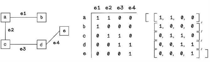
Figure 2.27 Representing a graph as an incidence matrix

Adjacency list

An adjacency list uses linked lists in which the size of the initial list is the number of nodes in the graph and each value represents the connected nodes for a specific node. An adjacency list can be used to represent both directed and undirected graphs (figure 2.28).

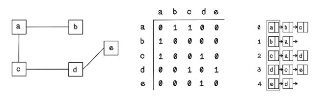
Figure 2.28 Representing a graph as an adjacency list

Graphs are also interesting and useful data structures because they can easily be represented as mathematical equations, which are the backing for all algorithms we use. You can find more information about this topic throughout the book.

Summary of search fundamentals