This chapter covers

• Understanding the inspiration and intuition of artificial neural networks

• Identifying problems that can be solved with artificial neural networks

• Understanding and implementing forward propagation using a trained network

• Understanding and implementing backpropagation to train a network

• Designing artificial neural network architectures to tackle different problems

What are artificial neural networks?

Artificial neural networks (ANNs) are powerful tools in the machine learning toolkit, used in a variety of ways to accomplish objectives such as image recognition, natural language processing, and game playing. ANNs learn in a similar way to other machine learning algorithms: by using training data. They are best suited to unstructured data where it’s difficult to understand how features relate to one another. This chapter covers the inspiration of ANNs; it also shows how the algorithm works and how ANNs are designed to solve different problems.

To gain a clear understanding of how ANNs fit into the bigger machine learning landscape, we should review the composition and categorization of machine learning algorithms. Deep learning is the name given to algorithms that use ANNs in varying architectures to accomplish an objective. Deep learning, including ANNs, can be used to solve supervised learning, unsupervised learning, and reinforcement learning problems. Figure 9.1 shows how deep learning relates to ANNs and other machine learning concepts.

Figure 9.1 A map describing the flexibility of deep learning and ANNs

ANNs can be seen as just another model in the machine learning life cycle (chapter 8). Figure 9.2 recaps that life cycle. A problem needs to be identified; that data needs to be collected, understood, and prepared; and the ANN model will be tested and improved if necessary.

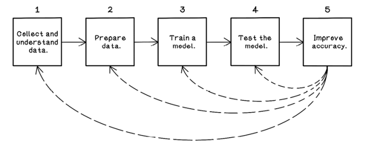
Figure 9.2 A workflow for machine learning experiments and projects

Now that we have an idea of how ANNs fit into the abstract machine learning landscape and know that an ANN is another model that is trained in the life cycle, let’s explore the intuition and workings of ANNs. Like genetic algorithms and swarm-intelligence algorithms, ANNs are inspired by natural phenomena—in this case, the brain and nervous system. The nervous system is a biological structure that allows us to feel sensations and is the basis of how our brains operate. We have nerves across our entire bodies and neurons that behave similarly in our brains.

Neural networks consist of interconnected neurons that pass information by using electrical and chemical signals. Neurons pass information to other neurons and adjust information to accomplish a specific function. When you grab a cup and take a sip of water, millions of neurons process the intention of what you want to do, the physical action to accomplish it, and the feedback to determine whether you were successful. Think about little children learning to drink from a cup. They usually start out poorly, dropping the cup a lot. Then they learn to grab it with two hands. Gradually, they learn to grab the cup with a single hand and take a sip without any problems. This process takes months. What’s happening is that their brains and nervous systems are learning through practice or training. Figure 9.3 depicts a simplified model of receiving inputs (stimuli), processing them in a neural network, and providing outputs (response).

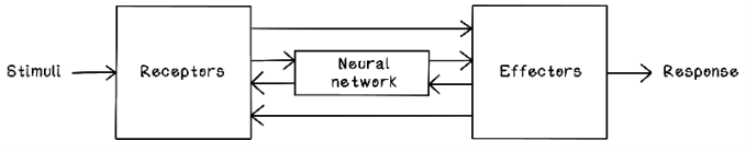
Figure 9.3 A simplified model of a biological neural system

Simplified, a neuron (figure 9.4) consists of dendrites that receive signals from other neurons; a cell body and a nucleus that activates and adjusts the signal; an axon that passes the signal to other neurons; and synapses that carry, and in the process adjust, the signal before it is passed to the next neuron’s dendrites. Through approximately 90 billion neurons working together, our brains can function at the high level of intelligence that we know.

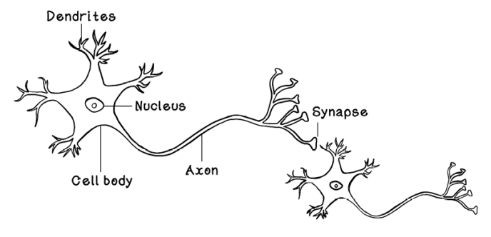
Figure 9.4 The general composition of neurons

Although ANNs are inspired by biological neural networks and use many of the concepts that are observed in these systems, ANNs are not identical representations of biological neural systems. We still have a lot to learn about the brain and nervous system.

The Perceptron: A representation of a neuron

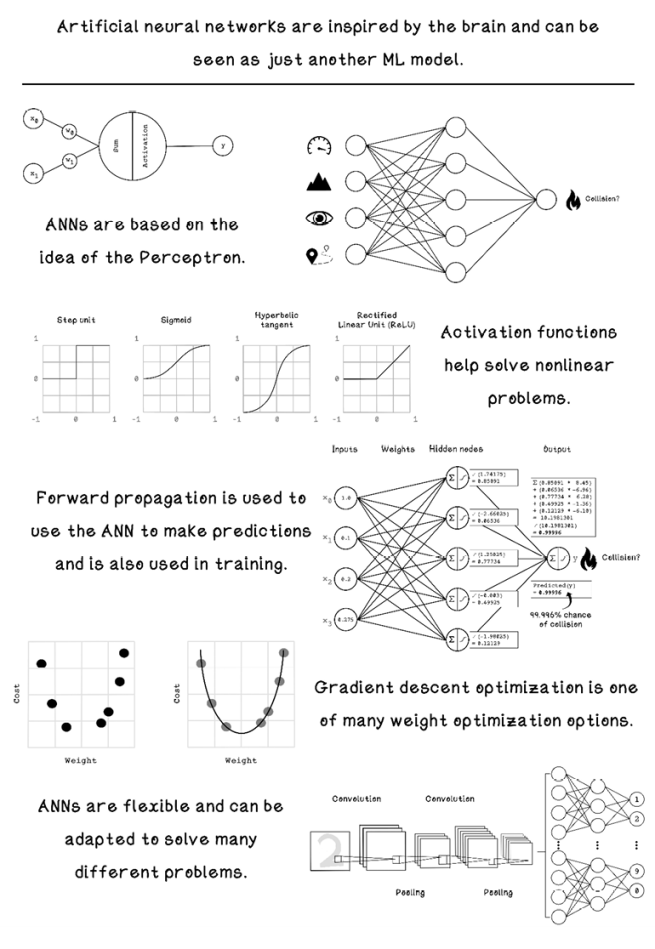
The neuron is the fundamental concept that makes up the brain and nervous system. As mentioned earlier, it accepts many inputs from other neurons, processes those inputs, and transfers the result to other connected neurons. ANNs are based on the fundamental concept of the Perceptron—a logical representation of a single biological neuron.

Like neurons, the Perceptron receives inputs (like dendrites), alters these inputs by using weights (like synapses), processes the weighted inputs (like the cell body and nucleus), and outputs a result (like axons). The Perceptron is loosely based on a neuron. You may notice that the synapses are depicted after the dendrites, representing the influence of synapses on incoming inputs. Figure 9.5 depicts the logical architecture of the Perceptron.

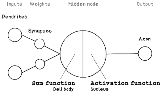
Figure 9.5 Logical architecture of the Perceptron

The components of the Perceptron are described by variables that are useful in calculating the output. Weights modify the inputs; that value is processed by a hidden node; and finally, the result is provided as the output.

Here is a brief description of the components of the Perceptron:

• Inputs—Describe the input values. In a neuron, these values would be an input signal.

• Weights—Describe the weights on each connection between an input and the hidden node. Weights influence the intensity of an input and result in a weighted input. In a neuron, these connections would be the synapses.

• Hidden node (sum and activation)—Sums the weighted input values and then applies an activation function to the summed result. An activation function determines the activation/output of the hidden node/neuron.

• Output—Describes the final output of the Perceptron.

To understand the workings of the Perceptron, we will examine the use of one by revisiting the apartment-hunting example from chapter 8. Suppose that we are real estate agents trying to determine whether a specific apartment will be rented within a month, based on the size of the apartment and the price of the apartment. Assume that a Perceptron has already been trained, meaning that the weights for the Perceptron have already been adjusted. We explore the way Perceptions and ANNs are trained later in this chapter; for now, understand that the weights encode relationships among the inputs by adjusting the strength of inputs.

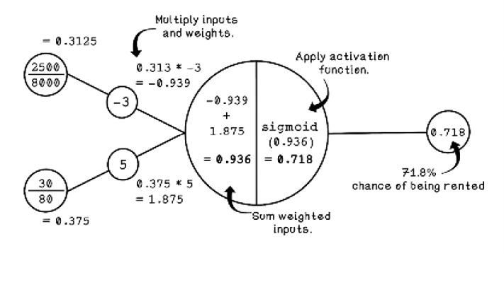
Figure 9.6 shows how we can use a pretrained Perceptron to classify whether an apartment will be rented. The inputs represent the price of a specific apartment and the size of that apartment. We’re also using the maximum price and size to scale the inputs ($8,000 for maximum price and 80 square meters for maximum size). For more about scaling data, see the next section.

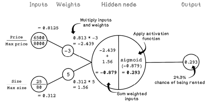
Figure 9.6 An example of using a trained Perceptron

Notice that the price and size are the inputs and that the predicted chance of the apartment being rented is the output. The weights are key to achieving the prediction. Weights are the variables in the network that learn relationships among inputs. The summation and activation functions are used to process the inputs multiplied by the weights to make a prediction.

Notice that we’re using an activation function called the sigmoid function. Activation functions play a critical role in the Perceptron and ANNs. In this case, the activation function is helping us solve a linear problem. But when we look at ANNs in the next section, we will see how activation functions are useful for receiving inputs to solve nonlinear problems. Figure 9.7 describes the basics of linear problems.

The sigmoid function results in an S curve between 0 and 1, given inputs between 0 and 1. Because the sigmoid function allows changes in x to result in small changes in y, it allows for gradual learning. When we get to the deeper workings of ANNs later in this chapter, we will see how this function helps solve nonlinear problems as well.

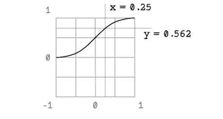
Figure 9.7 The sigmoid function

Let’s take a step back and look at the data that we’re using for the Perceptron. Understanding the data related to whether an apartment was sold is important for understanding what the Perceptron is doing. Figure 9.8 illustrates the examples in the dataset, including the price and size of each apartment. Each apartment is labeled as one of two classes: rented or not rented. The line separating the two classes is the function described by the Perceptron.

Figure 9.8 Example of a linear classification problem

Although the Perceptron is useful for solving linear problems, it cannot solve nonlinear problems. If a dataset cannot be classified by a straight line, the Perceptron will fail.

ANNs use the concept of the Perceptron at scale. Many neurons similar to the Perceptron work together to solve nonlinear problems in many dimensions. Note that the activation function used influences the learning capabilities of the ANN.

Exercise: Calculate the output of the following input for the Perceptron

Using your knowledge of how the Perceptron works, calculate the output for the following:

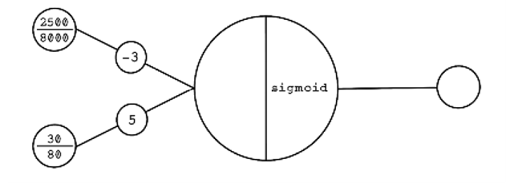
Solution: Calculate the output of the following input for the Perceptron

Defining artificial neural networks

The Perceptron is useful for solving simple problems, but as the dimensions of the data increases, it becomes less feasible. ANNs use the principles of the Perceptron and apply them to many hidden nodes as opposed to a single one.

To explore the workings of multi-node ANNs, consider an example dataset related to car collisions. Suppose that we have data from several cars at the moment that an unforeseen object enters the path of their movement. The dataset contains features related to the conditions and whether a collision occurred, including the following:

• Speed—The speed at which the car was traveling before encountering the object

• Terrain quality—The quality of the road on which the car was traveling before encountering the object

• Degree of vision—The driver’s degree of vision before the car encountered the object

• Total experience—The total driving experience of the driver of the car

• Collision occurred?—Whether a collision occurred or not

Given this data, we want to train a machine learning model—namely, an ANN—to learn the relationship between the features that contribute to a collision, as shown in table 9.1.

Table 9.1 Car collision dataset

	Speed	Terrain quality	Degree of vision	Total experience	Collision occurred?
1	65 km/h	5/10	180°	80,000 km	No
2	120 km/h	1/10	72°	110,000 km	Yes
3	8 km/h	6/10	288°	50,000 km	No
4	50 km/h	2/10	324°	1,600 km	Yes
5	25 km/h	9/10	36°	160,000 km	No
6	80 km/h	3/10	120°	6,000 km	Yes
7	40 km/h	3/10	360°	400,000 km	No

An example ANN architecture can be used to classify whether a collision will occur based on the features we have. The features in the dataset must be mapped as inputs to the ANN, and the class that we are trying to predict is mapped as the output of the ANN. In this example, the input nodes are speed, terrain quality, degree of vision, and total experience; the output node is whether a collision happened (figure 9.9).

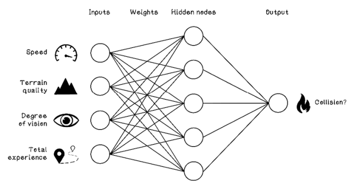
Figure 9.9 Example ANN architecture for the car-collision example

As with the other machine learning algorithms that we’ve worked through, preparing data is important for making an ANN classify data successfully. The primary concern is representing data in comparable ways. As humans, we understand the concept of speed and degree of vision, but the ANN doesn’t have this context. Directly comparing 65 km/h and 36-degree vision doesn’t make sense for the ANN, but comparing the ratio of speed with the degree of vision is useful. To accomplish this task, we need to scale our data.

A common way to scale data so that it can be compared is to use the min-max scaling approach, which aims to scale data to values between 0 and 1. By scaling all the data in a dataset to be consistent in format, we make the different features comparable. Because ANNs do not have any context about the raw features, we also remove bias with large input values. As an example, 1,000 seems to be much larger than 65, but 1,000 in the context of total driving experience is poor, and 65 in the context of driving speed is significant. Min-max scaling represents these pieces of data with the correct context by taking into account the minimum and maximum possible values for each feature.

Here are the minimum and maximum values selected for the features in the car-collision data:

• Speed—The minimum speed is 0, which means that the car is not moving. We will use the maximum speed of 120, because 120 km/h is the maximum legal speed limit in most places around the world. We will assume that the driver follows the rules.

• Terrain quality—Because the data is already in a rating system, the minimum value is 0, and the maximum value is 10.

• Degree of vision—We know that the total field of view in degrees is 360. So the minimum value is 0, and the maximum value is 360.

• Total experience—The minimum value is 0 if the driver has no experience. We will subjectively make the maximum value 400,000 for driving experience. The rationale is that if a driver has 400,000 km of driving experience, we consider that driver to be highly competent, and any further experience doesn’t matter.

Min-max scaling uses the minimum and maximum values for a feature and finds the percentage of the actual value for the feature. The formula is simple: subtract the minimum from the value, and divide the result by the minimum subtracted from the maximum. Figure 9.10 illustrates the min-max scaling calculation for the first row of data in the car-collision example:

	Speed	Terrain quality	Degree of vision	Total experience	Collision occurred?
1	65 km/h	5/10	180°	80,000 km	No

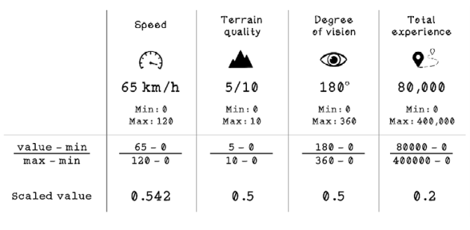
Figure 9.10 Min-max scaling example with car collision data

Notice that all the values are between 0 and 1 and can be compared equally. The same formula is applied to all the rows in the dataset to ensure that every value is scaled. Note that for the value for the “Collision occurred?” feature, Yes is replaced with 1, and No is replaced with 0. Table 9.2 depicts the scaled car-collision data.

Table 9.2 Car collision dataset scaled

	Speed	Terrain quality	Degree of vision	Total experience	Collision occurred?
1	0.542	0.5	0.5	0.200	0
2	1.000	0.1	0.2	0.275	1
3	0.067	0.6	0.8	0.125	0
4	0.417	0.2	0.9	0.004	1
5	0.208	0.9	0.1	0.400	0
6	0.667	0.3	0.3	0.015	1
7	0.333	0.3	1.0	1.000	0

Pseudocode

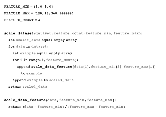
The code for scaling the data follows the logic and calculations for min-max scaling identically. We need the minimums and maximums for each feature, as well as the total number of features in our dataset. The scale_dataset function uses these parameters to iterate over every example in the dataset and scale the value by using the scale_data_feature function:

Now that we have prepared the data in a way that is suitable for an ANN to process, let’s explore the architecture of a simple ANN. Remember that the features used to predict a class are the input nodes, and the class that is being predicted is the output node.

Figure 9.11 shows an ANN with one hidden layer, which is the single vertical layer in the figure, with five hidden nodes. These layers are called hidden layers because they are not directly observed from outside the network. Only the inputs and outputs are interacted with, which leads to the perception of ANNs as being black boxes. Each hidden node is similar to the Perceptron. A hidden node takes inputs and weights and then computes the sum and an activation function. Then the results of each hidden node are processed by a single output node.

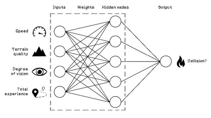
Figure 9.11 Example ANN architecture for the car-collision problem

Before we consider the calculations and computation of an ANN, let’s try to dig intuitively into what the network weights are doing at a high level. Because a single hidden node is connected to every input node but every connection has a different weight, independent hidden nodes might be concerned with specific relationships among two or more input nodes.

Figure 9.12 depicts a scenario in which the first hidden node has strong weightings on the connections to terrain quality and degree of vision but weak weightings on the connections to speed and total experience. This specific hidden node is concerned with the relationship between terrain quality and degree of vision. It might gain an understanding of the relationship between these two features and how it influences whether collisions happen; poor terrain quality and poor degree of vision, for example, might influence the likelihood of collisions more than good terrain quality and an average degree of vision. These relationships are usually more intricate than this simple example.

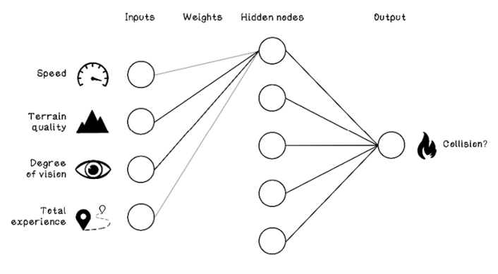
Figure 9.12 Example of a hidden node comparing terrain quality and degree of vision

In figure 9.13, the second hidden node might have strong weightings on the connections to terrain quality and total experience. Perhaps there is a relationship among different terrain qualities and variance in total driving experience that contributes to collisions.

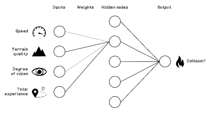
Figure 9.13 Example of a hidden node comparing terrain quality and total experience

The nodes in a hidden layer can be conceptually compared with the analogy of ants discussed in chapter 6. Individual ants fulfill small tasks that are seemingly insignificant, but when the ants act as a colony, intelligent behavior emerges. Similarly, individual hidden nodes contribute to a greater goal in the ANN.

By analyzing the figure of the car-collision ANN and the operations within it, we can describe the data structures required for the algorithm:

• Input nodes—The input nodes can be represented by a single array that stores the values for a specific example. The array size is the number of features in the dataset that are being used to predict a class. In the car-collision example, we have four inputs, so the array size is 4.

• Weights—The weights can be represented by a matrix (a 2D array), because each input node has a connection to each hidden node and each input node has five connections. Because there are 4 input nodes with 5 connections each, the ANN has 20 weights toward the hidden layer and 5 toward the output layer, because there are 5 hidden nodes and 1 output node.

• Hidden nodes—The hidden nodes can be represented by a single array that stores the results of activation of each respective node.

• Output node—The output node is a single value representing the predicted class of a specific example or the chance that the example will be in a specific class. The output might be 1 or 0, indicating whether a collision occurred; or it could be something like 0.65, indicating a 65% chance that the example resulted in a collision.

Pseudocode

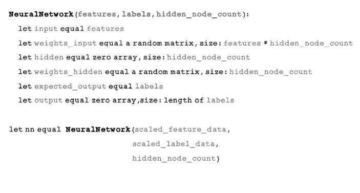
The next piece of pseudocode describes a class that represents a neural network. Notice that the layers are represented as properties of the class and that all the properties are arrays, with the exception of the weights, which are matrices. An output property represents the predictions for the given examples, and an expected_output property is used during the training process:

Forward propagation: Using a trained ANN

A trained ANN is a network that has learned from examples and adjusted its weights to best predict the class of new examples. Don’t panic about how the training happens and how the weights are adjusted; we will tackle this topic in the next section. Understanding forward propagation will assist us in grasping backpropagation (how weights are trained).

Now that we have a grounding in the general architecture of ANNs and the intuition of what nodes in the network might be doing, let’s walk through the algorithm for using a trained ANN (figure 9.14).

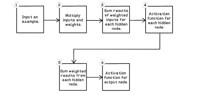
Figure 9.14 Life cycle of forward propagation in an ANN

As mentioned previously, the steps involved in calculating the results for the nodes in an ANN are similar to the Perceptron. Similar operations are performed on many nodes that work together; this addresses the Perceptron’s flaws and is used to solve problems that have more dimensions. The general flow of forward propagation includes the following steps:

1. Input an example—Provide a single example from the dataset for which we want to predict the class.

2. Multiply inputs and weights—Multiply every input by each weight of its connection to hidden nodes.

3. Sum results of weighted inputs for each hidden node—Sum the results of the weighted inputs.

4. Activation function for each hidden node—Apply an activation function to the summed weighted inputs.

5. Sum results of weighted outputs of hidden nodes to the output node—Sum the weighted results of the activation function from all hidden nodes.

6. Activation function for output node—Apply an activation function to the summed weighted hidden nodes.

For the purpose of exploring forward propagation, we will assume that the ANN has been trained and the optimal weights in the network have been found. Figure 9.15 depicts the weights on each connection. The first box next to the first hidden node, for example, has the weight 3.35, which is related to the Speed input node; the weight -5.82 is related to the Terrain Quality input node; and so on.

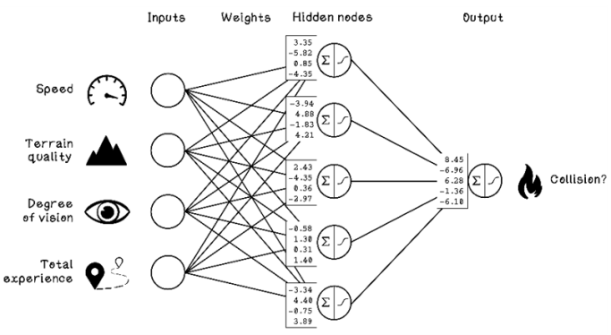
Figure 9.15 Example of weights in a pretrained ANN

Because the neural network has been trained, we can use it to predict the chance of collisions by providing it with a single example. Table 9.3 serves as a reminder of the scaled dataset that we are using.

Table 9.3 Car collision dataset scaled

	Speed	Terrain quality	Degree of vision	Total experience	Collision occurred?
1	0.542	0.5	0.5	0.200	0
2	1.000	0.1	0.2	0.275	1
3	0.067	0.6	0.8	0.125	0
4	0.417	0.2	0.9	0.004	1
5	0.208	0.9	0.1	0.400	0
6	0.667	0.3	0.3	0.015	1
7	0.333	0.3	1.0	1.000	0

If you’ve ever looked into ANNs, you may have noticed some potentially frightening mathematical notations. Let’s break down some of the concepts that can be represented mathematically.

The inputs of the ANN are denoted by X. Every input variable will be X subscripted by a number. Speed is X0, Terrain Quality is X1, and so on. The output of the network is denoted by y, and the weights of the network are denoted by W. Because we have two layers in the ANN—a hidden layer and an output layer—there are two groups of weights. The first group is superscripted by W0, and the second group is W1. Then each weight is denoted by the nodes to which it is connected. The weight between the Speed node and the first hidden node is W00,0, and the weight between the Terrain Quality node and the first hidden node is W01,0. These denotations aren’t necessarily important for this example, but understanding them now will support future learning.

Figure 9.16 shows how the following data is represented in an ANN:

	Speed	Terrain quality	Degree of vision	Total experience	Collision occurred?
1	0.542	0.5	0.5	0.200	0

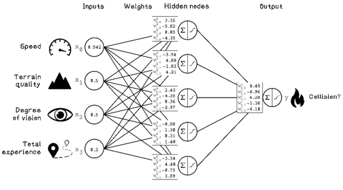
Figure 9.16 Mathematical denotation of an ANN

As with the Perceptron, the first step is calculating the weighted sum of the inputs and the weight of each hidden node. In figure 9.17, each input is multiplied by each weight and summed for every hidden node.

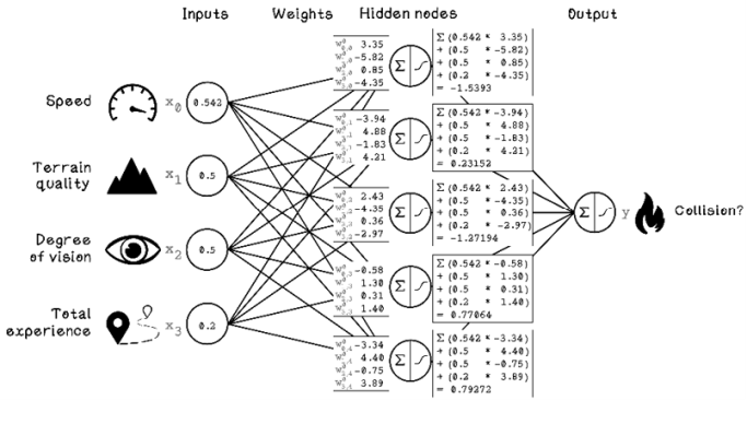
Figure 9.17 Weighted sum calculation for each hidden node

The next step is calculating the activation of each hidden node. We are using the sigmoid function, and the input for the function is the weighted sum of the inputs calculated for each hidden node (figure 9.18).

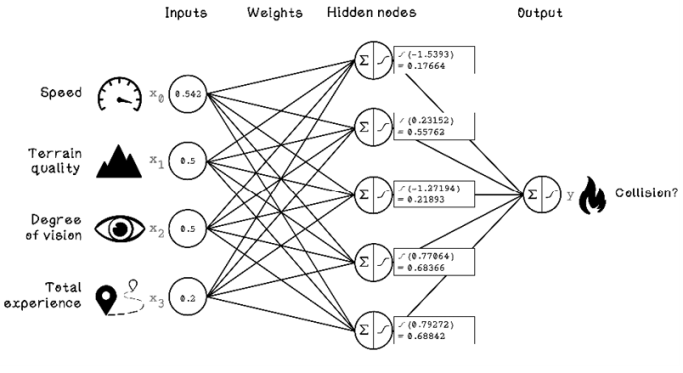
Figure 9.18 Activation function calculation for each hidden node

Now we have the activation results for each hidden node. When we mirror this result back to neurons, the activation results represent the activation intensity of each neuron. Because different hidden nodes may be concerned with different relationships in the data through the weights, the activations can be used in conjunction to determine an overall activation that represents the chance of a collision, given the inputs.

Figure 9.19 depicts the activations for each hidden node and the weights from each hidden node to the output node. To calculate the final output, we repeat the process of calculating the weighted sum of the results from each hidden node and applying the sigmoid activation function to that result.

Note The sigma symbol (Σ) in the hidden nodes depicts the sum operation.

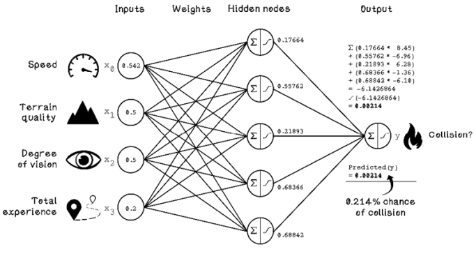
Figure 9.19 Final activation calculation for the output node

We have calculated the output prediction for our example. The result is 0.00214, but what does this number mean? The output is a value between 0 and 1 that represents the probability that a collision will occur. In this case, the output is 0.214 percent (0.00214 × 100), indicating that the chance of a collision is almost 0.

The following exercise uses another example from the dataset.

Exercise: Calculate the prediction for the example BY using forward propagation with the following ANN

	Speed	Terrain quality	Degree of vision	Total experience	Collision occurred?
2	1.000	0.1	0.2	0.275	1

Solution: Calculate the prediction for the example BY using forward propagation with the following ANN

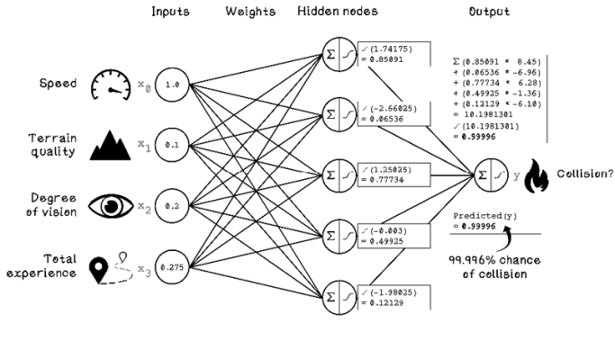
When we run this example through our pretrained ANN, the output is 0.99996, or 99.996 percent, so there is an extremely high chance that a collision will occur. By applying some human intuition to this single example, we can see why a collision is likely. The driver was traveling at the maximum legal speed, on the poorest-quality terrain, with a poor field of vision.

Pseudocode

One of the important functions for activation in our example is the sigmoid function. This method describes the mathematical function that represents the S curve:

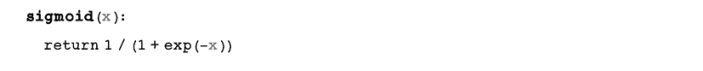
b Exp is a mathematical constant called Euler’s number, approximately 2.71828.

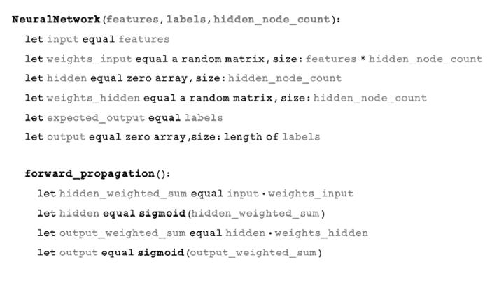
Notice that the same neural network class defined earlier in the chapter is described in the following code. This time, a forward_propagation function is included. This function sums the input and weights between input and hidden nodes, applies the sigmoid function to each result, and stores the output as the result for the nodes in the hidden layer. This is done for the hidden node output and weights to the output node as well:

Backpropagation: Training an ANN

Understanding how forward propagation works is useful for understanding how ANNs are trained, because forward propagation is used in the training process. The machine learning life cycle and principles covered in chapter 8 are important for tackling backpropagation in ANNs. An ANN can be seen as another machine learning model. We still need to have a question to ask. We’re still collecting and understanding data in the context of the problem, and we need to prepare the data in a way that is suitable for the model to process.

We need a subset of data for training and a subset of data for testing how well the model performs. Also, we will be iterating and improving through collecting more data, preparing it differently, or changing the architecture and configuration of the ANN.

Training an ANN consists of three main phases. Phase A involves setting up the ANN architecture, including configuring the inputs, outputs, and hidden layers. Phase B is forward propagation. And phase C is backpropagation, which is where the training happens (figure 9.20).

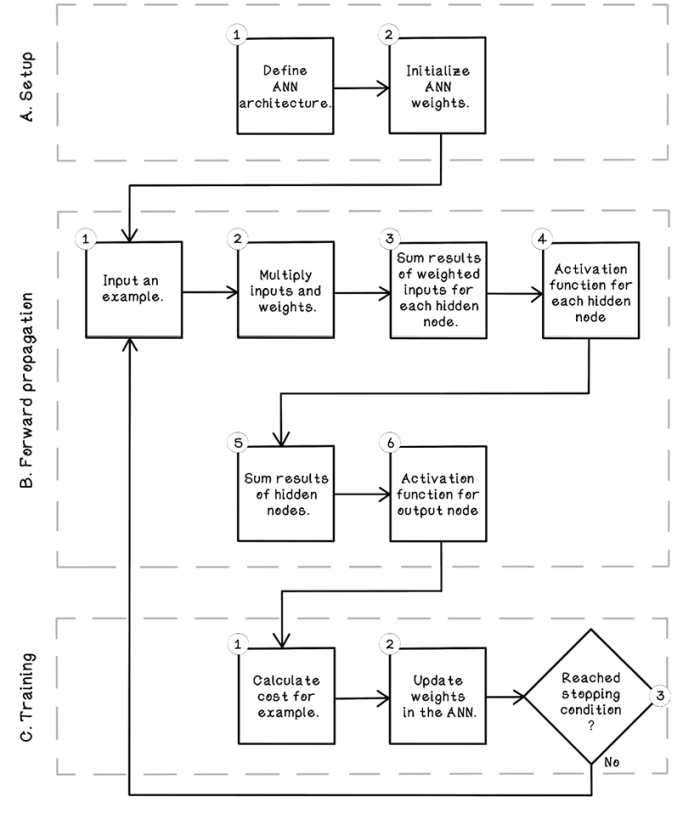
Figure 9.20 Life cycle of training an ANN

Phase A, Phase B, and Phase C describe the phases and operations involved in the back-propagation algorithm.

Phase A: Setup

1. Define ANN architecture. This step involves defining the input nodes, the output nodes, the number of hidden layers, the number of neurons in each hidden layer, the activation functions used, and more.

2. Initialize ANN weights. The weights in the ANN must be initialized to some value. We can take various approaches. The key principle is that the weights will be adjusted constantly as the ANN learns from training examples.

Phase B: Forward propagation

This process is the same one that we covered in Phase A. The same calculations are carried out. The predicted output, however, will be compared with the actual class for each example in the training set to train the network.

Phase C: Training

1. Calculate cost. Following from forward propagation, the cost is the difference between the predicted output and the actual class for the examples in the training set. The cost effectively determines how bad the ANN is at predicting the class of examples.

2. Update weights in the ANN. The weights of the ANN are the only things that can be adjusted by the network itself. The architecture and configurations that we defined in phase A don’t change during training the network. The weights essentially encode the intelligence of the network. Weights are adjusted to be larger or smaller, affecting the strength of the inputs.

3. Define a stopping condition. Training cannot happen indefinitely. As with many of the algorithms explored in this book, a sensible stopping condition needs to be determined. If we have a large dataset, we might decide that we will use 500 examples in our training dataset over 1,000 iterations to train the ANN. In this example, the 500 examples will be passed through the network 1,000 times, and the weights will be adjusted in every iteration.

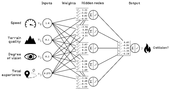
When we worked through forward propagation, the weights were already defined because the network was pretrained. Before we start training the network, we need to initialize the weights to some value, and the weights need to be adjusted based on training examples. One approach to initializing weights is to choose random weights from a normal distribution.

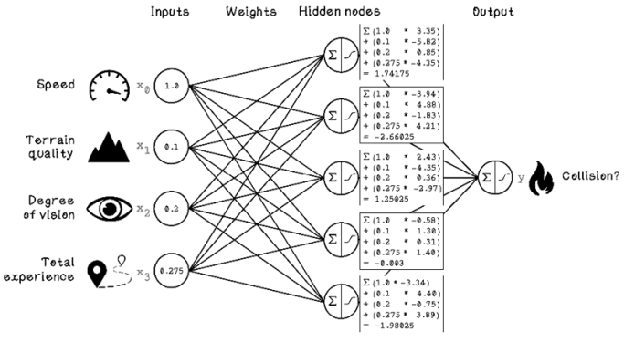
Figure 9.21 illustrates the randomly generated weights for our ANN. It also shows the calculations for forward propagation for the hidden nodes, given a single training example. The first example input used in the forward propagation section is used here to highlight the differences in output, given different weights in the network.

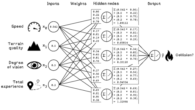
Figure 9.21 Example initial weights for an ANN

The next step is forward propagation (figure 9.22). The key change is checking the difference between the obtained prediction and the actual class.

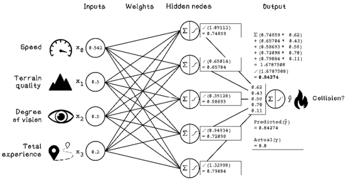
Figure 9.22 Example of forward propagation with randomly initialized weights

By comparing the predicted result with the actual class, we can calculate a cost. The cost function that we will use is simple: subtract the predicted output from the actual output. In this example, 0.84274 is subtracted from 0.0, and the cost is -0.84274. This result indicates how incorrect the prediction was and can be used to adjust the weights in the ANN. Weights in the ANN are adjusted slightly every time a cost is calculated. This happens thousands of times using training data to determine the optimal weights for the ANN to make accurate predictions. Note that training too long on the same set of data can lead to overfitting, described in chapter 8.

Here is where some potentially unfamiliar math comes into play: the Chain Rule. Before we use the Chain Rule, let’s gain some intuition about what the weights mean and how adjusting them improves the ANN’s performance.

If we plot possible weights against their respective cost on a graph, we find some function that represents the possible weights. Some points on the function yield a lower cost, and other points yield a higher cost. We are seeking points that minimize cost (figure 9.23).

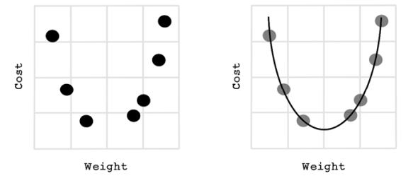
Figure 9.23 Weight versus cost plotted

A useful tool from the field of calculus, called gradient descent, can help us move the weight closer to the minimum value by finding the derivative. The derivative is important because it measures the sensitivity to change for that function. For example, velocity might be the derivative of an object’s position with respect to time; and acceleration is the derivative of the object’s velocity with respect to time. Derivatives can find the slope at a specific point in the function. Gradient descent uses the knowledge of the slope to determine which way to move and by how much. Figures 9.24 and 9.25 describe how the derivatives and slope indicate the direction of the minimums.

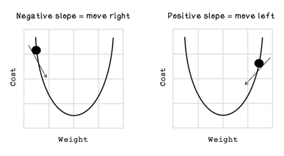
Figure 9.24 Derivatives’ slopes and direction of minimums

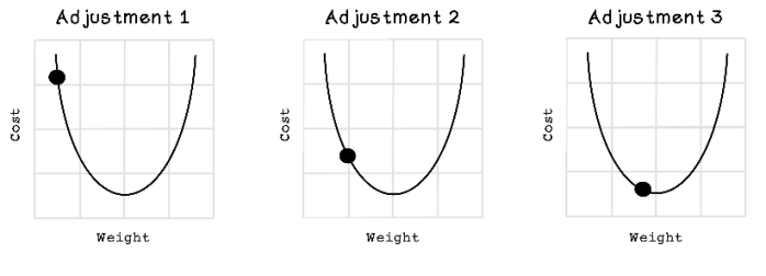
Figure 9.25 Example of adjusting a weight by using gradient descent

When we look at one weight in isolation, it may seem trivial to find a value that minimizes the cost, but many weights being balanced affect the cost of the overall network. Some weights may be close to their optimal points in reducing cost, and others may not, even though the ANN performs well.

Because many functions comprise the ANN, we can use the Chain Rule. The Chain Rule is a theorem from the field of calculus that calculates the derivative of a composite function. A composite function uses a function g as the parameter for a function f to produce a function h, essentially using a function as a parameter of another function.

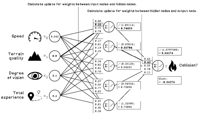
Figure 9.26 illustrates the use of the Chain Rule in calculating the update value for weights in the different layers of the ANN.

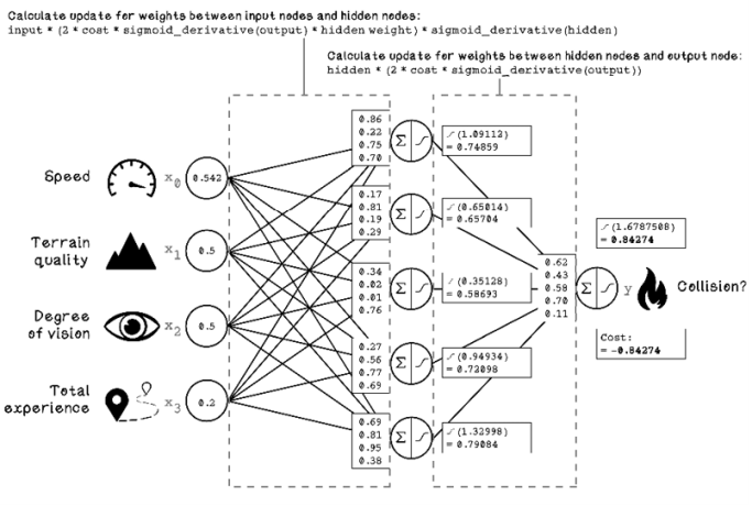
Figure 9.26 Formula for calculating weight updates with the Chain Rule

We can calculate the weight update by plugging the respective values into the formula described. The calculations look scary, but pay attention to the variables being used and their role in the ANN. Although the formula looks complex, it uses the values that we have already calculated (figure 9.27).

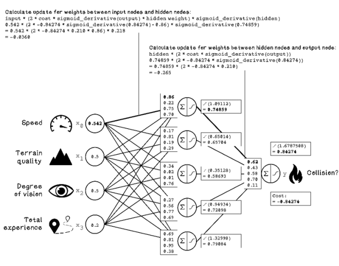
Figure 9.27 Weight-update calculation with the Chain Rule

Here’s a closer look at the calculations used in figure 9.27:

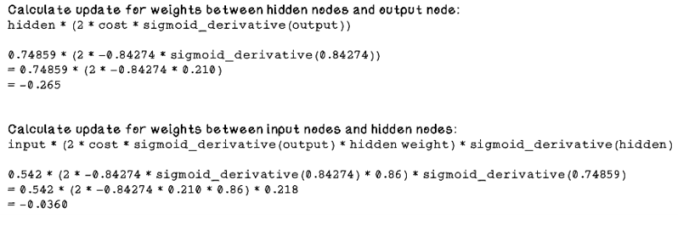
Now that the update values are calculated, we can apply the results to the weights in the ANN by adding the update value to the respective weights. Figure 9.28 depicts the application of the weight-update results to the weights in the different layers.

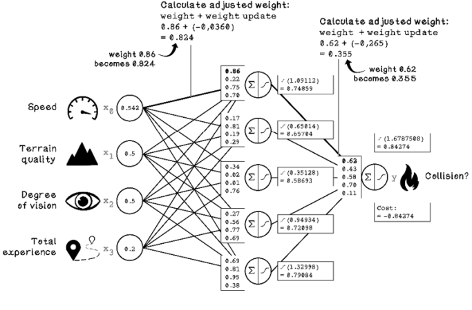
Figure 9.28 Example of the final weight-update for the ANN

Exercise: Calculate the new weights for the highlighted weights

Solution: Calculate the new weights for the highlighted weights

The problem that the Chain Rule is solving may remind you of the drone problem example in chapter 7. Particle-swarm optimization is effective for finding optimal values in high-dimensional spaces such as this one, which has 25 weights to optimize. Finding the weights in an ANN is an optimization problem. Gradient descent is not the only way to optimize weights; we can use many approaches, depending on the context and problem being solved.

Pseudocode

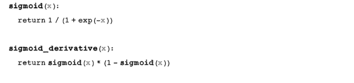
The derivative is important in the backpropagation algorithm. The following piece of pseudocode revisits the sigmoid function and describes the formula for its derivative, which we need to adjust weights:

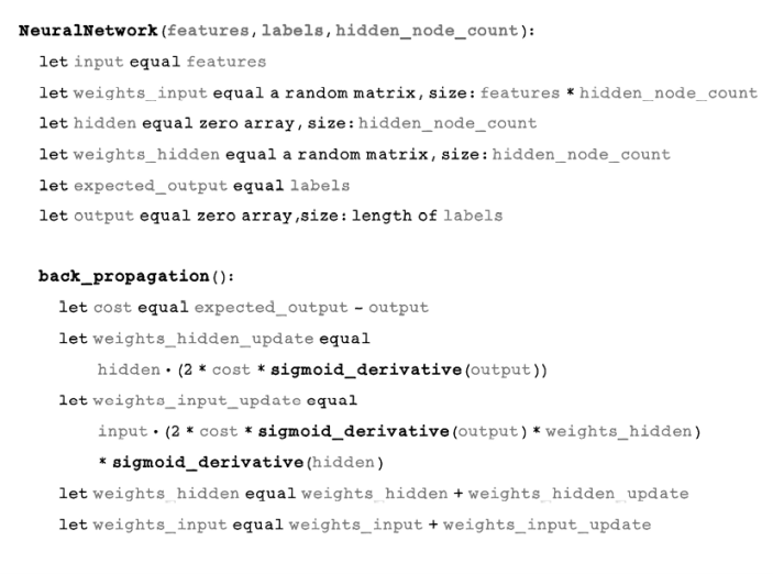
We revisit the neural network class, this time with a backpropagation function that computes the cost, the amount by which weights should be updated by using the Chain Rule, and adds the weight-update results to the existing weights. This process will compute the change for each weight given the cost. Remember that cost is calculated by using the example features, predicted output, and expected output. The difference between the predicted output and expected output is the cost:

Because we have a class that represents a neural network, functions to scale data, and functions for forward propagation and backpropagation, we can piece this code together to train a neural network.

Pseudocode

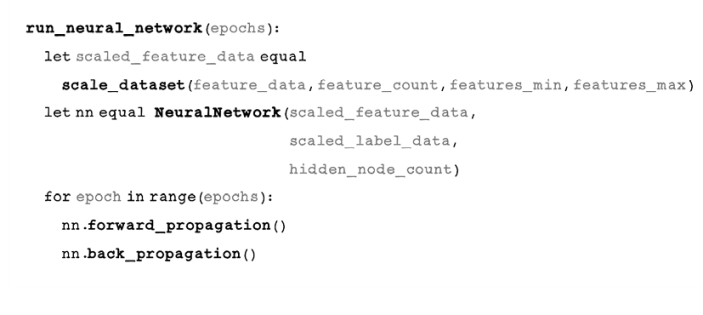
In this piece of pseudocode, we have a run_neural_network function that accepts epochs as an input. This function scales the data and creates a new neural network with the scaled data, labels, and number of hidden nodes. Then the function runs forward_propagation and back_propagation for the specified number of epochs:

Options for activation functions

This section aims to provide some intuition about activation functions and their properties. In the examples of the Perceptron and ANN, we used a sigmoid function as the activation function, which was satisfactory for the examples that we were working with. Activation functions introduce nonlinear properties to the ANN. If we do not use an activation function, the neural network will behave similarly to linear regression as described in chapter 8. Figure 9.29 describes some commonly used activation functions.

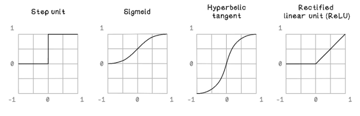
Figure 9.29 Commonly used activation functions

Different activation functions are useful in different scenarios and have different benefits:

• Step unit—The step unit function is used as a binary classifier. Given an input between -1 and 1, it outputs a result of exactly 0 or 1. A binary classifier is not useful for learning from data in a hidden layer, but it can be used in the output layer for binary classification. If we want to know whether something is a cat or a dog, for example, 0 could indicate cat, and 1 could indicate dog.

• Sigmoid—The sigmoid function results in an S curve between 0 and 1, given an input between -1 and 1. Because the sigmoid function allows changes in x to result in small changes in y, it allows for learning and solving nonlinear problems. The problem sometimes experienced with the sigmoid function is that as values approach the extremes, derivative changes become tiny, resulting in poor learning. This problem is known as the vanishing gradient problem.

• Hyperbolic tangent—The hyperbolic tangent function is similar to the sigmoid function, but it results in values between -1 and 1. The benefit is that the hyperbolic tangent has steeper derivatives, which allows for faster learning. The vanishing gradient problem is also a problem at the extremes for this function, as with the sigmoid function.

• Rectified linear unit (ReLU)—The ReLU function results in 0 for input values between -1 and 0, and results in linearly increasing values between 0 and 1. In a large ANN with many neurons using the sigmoid or hyperbolic tangent function, all neurons activate all the time (except when they result in 0), resulting in lots of computation and many values being adjusted finely to find solutions. The ReLU function allows some neurons to not activate, which reduces computation and may find solutions faster.

The next section touches on some considerations for designing an ANN.

Designing artificial neural networks

Designing ANNs is experimental and dependent on the problem that is being solved. The architecture and configuration of an ANN usually change through trial and error as we attempt to improve the performance of the predictions. This section briefly lists the parameters of the architecture that we can change to improve performance or address different problems. Figure 9.30 illustrates an artificial neural network with a different configuration to the one seen throughout this chapter. The most notable difference is the introduction of a new hidden layer and the network now has two outputs.

Note As in most scientific or engineering problems, the answer to “What is the ideal ANN design?” is often “It depends.” Configuring ANNs requires a deep understanding of the data and the problem being solved. A clear-cut generalized blueprint for architectures and configurations doesn’t exist . . . yet.

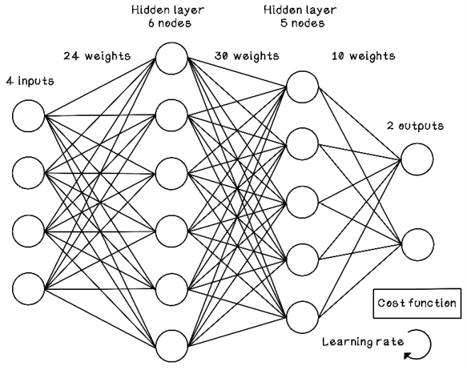
Figure 9.30 An example of a multilayer ANN with more than one output

Inputs and outputs

The inputs and outputs of an ANN are the fundamental parameters for use of the network. After an ANN model has been trained, the trained ANN model will potentially be used in different contexts and systems, and by different people. The inputs and outputs define the interface of the network. Throughout this chapter, we saw an example of an ANN with four inputs describing the features of a driving scenario and one output describing the likelihood of a collision. We may have a problem when the inputs and outputs mean different things, however. If we have a 16- by 16-pixel image that represents a handwritten digit, for example, we could use the pixels as inputs and the digit they represent as the output. The input would consist of 256 nodes representing the pixel values, and the output would consist of 10 nodes representing 0 to 9, with each result indicating the probability that the image is the respective digit.

Hidden layers and nodes

An ANN can consist of multiple hidden layers with varying numbers of nodes in each layer. Adding more hidden layers allows us to solve problems with higher dimensions and more complexity in the classification discrimination line. In the example in figure 9.8, a simple straight line classified data accurately. Sometimes, the line is nonlinear but fairly simple. But what happens when the line is a more-complex function with many curves potentially across many dimensions (which we can’t even visualize)? Adding more layers allows these complex classification functions to be found. The selection of the number of layers and nodes in an ANN usually comes down to experimentation and iterative improvement. Over time, we may gain intuition about suitable configurations, based on experiencing similar problems and solving them with similar configurations.

Weights

Weight initialization is important because it establishes a starting point from which the weight will be adjusted slightly over many iterations. Weights that are initialized to be too small lead to the vanishing gradient problem described earlier, and weights that are initialized to be too large lead to another problem, the exploding gradient problem—in which weights move erratically around the desired result.

Various weight-initialization schemes exist, each with its own pros and cons. A rule of thumb is to ensure that the mean of the activation results in a layer is 0—the mean of all results of the hidden nodes in a layer. Also, the variance of the activation results should be the same: the variability of the results from each hidden node should be consistent over several iterations.

Bias

We can use bias in an ANN by adding a value to the weighted sum of the input nodes or other layers in the network. A bias can shift the activation value of the activation function. A bias provides flexibility in an ANN and shifts the activation function left or right.

A simple way to understand bias is to imagine a line that always passes through 0,0 on a plane; we can influence this line to pass through a different intercept by adding +1 to a variable. This value will be based on the problem to be solved.

Activation functions

Earlier we covered the common activation functions used in ANNs. A key rule of thumb is to ensure that all nodes on the same layer use the same activation function. In multilayer ANNs, different layers may use different activation functions based on the problem to be solved. A network that determines whether loans should be granted, for example, might use the sigmoid function in the hidden layers to determine probabilities and a step function in the output to get a clear 0 or 1 decision.

Cost function and learning rate

We used a simple cost function in the example described earlier where the predicted output is subtracted from the actual expected output, but many cost functions exist. Cost functions influence the ANN greatly, and using the correct function for the problem and dataset at hand is important because it describes the goal for the ANN. One of the most common cost functions is mean square error, which is similar to the function used in the machine learning chapter (chapter 8). But cost functions must be selected based on understanding of the training data, size of the training data, and desired precision and recall measurements. As we experiment more, we should look into the cost function options.

Finally, the learning rate of the ANN describes how dramatically weights are adjusted during backpropagation. A slow learning rate may result in a long training process because weights are updated by tiny amounts each time, and a high learning rate might result in dramatic changes in the weights, making for a chaotic training process. One solution is to start with a fixed learning rate and to adjust that rate if the training stagnates and doesn’t improve the cost. This process, which would be repeated through the training cycle, requires some experimentation. Stochastic gradient descent is a useful tweak to the optimizer that combats these problems. It works similarly to gradient descent but allows weights to jump out of local minimums to explore better solutions.

Standard ANNs such as the one described in this chapter are useful for solving nonlinear classification problems. If we are trying to categorize examples based on many features, this ANN style is likely to be a good option.

That said, an ANN is not a silver bullet and shouldn’t be the go-to algorithm for anything. Simpler, traditional machine learning algorithms described in chapter 8 often perform better in many common use cases. Remember the machine learning life cycle. You may want to try several machine learning models during your iterations while seeking improvement.

Artificial neural network types and use cases

ANNs are versatile and can be designed to address different problems. Specific architectural styles of ANNs are useful for solving certain problems. Think of an ANN architectural style as being the fundamental configuration of the network. The examples in this section highlight different configurations.

Convolutional neural network

Convolutional neural networks (CNNs) are designed for image recognition. These networks can be used to find the relationships among different objects and unique areas within images. In image recognition, convolution operates on a single pixel and its neighbors within a certain radius. This technique is traditionally used for edge detection, image sharpening, and image blurring. CNNs use convolution and pooling to find relationships among pixels in an image. Convolution finds features in images, and pooling downsamples the “patterns” by summarizing features, allowing unique signatures in images to be encoded concisely through learning from multiple images (figure 9.31).

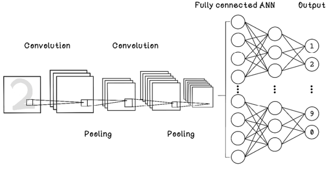
Figure 9.31 Simple example of a CNN

CNNs are used for image classification. If you’ve ever searched for an image online, you have likely interacted indirectly with a CNN. These networks are also useful for optical character recognition for extracting text data from an image. CNNs have been used in the medical industry for applications that detect anomalies and medical conditions via X-rays and other body scans.

Recurrent neural network

Whereas standard ANNs accept a fixed number of inputs, recurrent neural networks (RNNs) accept a sequence of inputs with no predetermined length. These inputs are like spoken sentences. RNNs have a concept of memory consisting of hidden layers that represent time; this concept allows the network to retain information about the relationships among the sequences of inputs. When we are training a RNN, the weights in the hidden layers throughout time are also influenced by backpropagation; multiple weights represent the same weight at different points in time (figure 9.32).

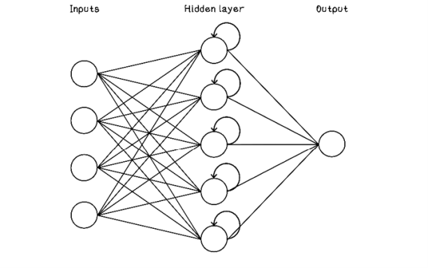
Figure 9.32 Simple example of a RNN

RNNs are useful in applications pertaining to speech and text recognition and prediction. Related use cases include autocompletion of sentences in messaging applications, translation of spoken language to text, and translation between spoken languages.

Generative adversarial network

A generative adversarial network (GAN) consists of a generator network and a discriminator network. For example, the generator creates a potential solution such as an image or a landscape, and a discriminator uses real images of landscapes to determine the realism or correctness of the generated landscape. The error or cost is fed back into the network to further improve its ability to generate convincing landscapes and determine their correctness. The term adversarial is key, as we saw with game trees in chapter 3. These two components are competing to be better at what they do and, through that competition, generate incrementally better solutions (figure 9.33).

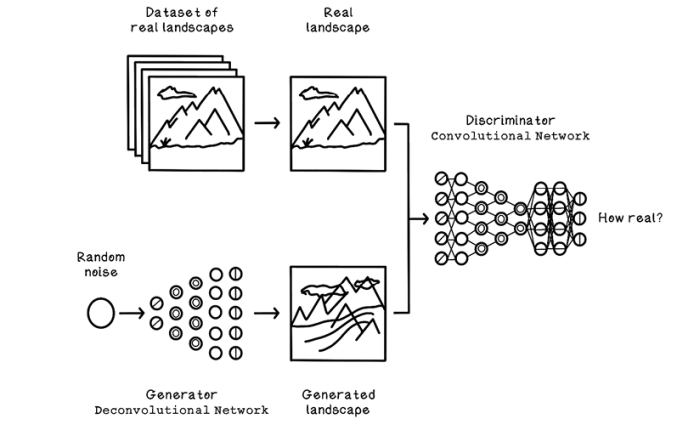
Figure 9.33 Simple example of a GAN

GANs are used to generate convincing fake videos (also known as deepfakes) of famous people, which raises concern about the authenticity of information in the media. GANs also have useful applications such as overlaying hairstyles on people’s faces. GANs have been used to generate 3D objects from 2D images, such as generating a 3D chair from a 2D picture. This use case may seem to be unimportant, but the network is accurately estimating and creating information from a source that is incomplete. It is a huge step in the advancement of AI and technology in general.

This chapter aimed to tie together the concepts of machine learning with the somewhat-mysterious world of ANNs. For further learning about ANNs and deep learning, try Grokking Deep Learning (Manning Publications); and for a practical guide to a framework for building ANNs, see Deep Learning with Python (Manning Publications).

Summary of artificial neural networks