This chapter covers

• Understanding and designing heuristics for guided search

• Identifying problems suited to being solved with guided search approaches

• Understanding and designing a guided search algorithm

• Designing a search algorithm to play a two-player game

Defining heuristics: Designing educated guesses

Now that we have an idea of how uninformed search algorithms work from chapter 2, we can explore how they can be improved by seeing more information about the problem. For this purpose, we use informed search. Informed search means that the algorithm has some context of the specific problem being solved. Heuristics are a way to represent this context. Often described as a rule of thumb, a heuristic is a rule or set of rules used to evaluate a state. It can be used to define criteria that a state must satisfy or measure the performance of a specific state. A heuristic is used when a clear method of finding an optimal solution is not possible. A heuristic can be interpreted as an educated guess in social terms and should be seen more as a guideline than as a scientific truth with respect to the problem that is being solved.

When you’re ordering a pizza at a restaurant, for example, your heuristic of how good it is may be defined by the ingredients and type of base used. If you enjoy extra tomato sauce, extra cheese, mushrooms, and pineapple on a thick base with crunchy crust, a pizza that includes more of these attributes will be more appealing to you and achieve a better score for your heuristic. A pizza that contains fewer of those attributes will be less appealing to you and achieve a poorer score.

Another example is writing algorithms to solve a GPS routing problem. The heuristic may be “Good paths minimize time in traffic and minimize distance traveled” or “Good paths minimize toll fees and maximize good road conditions.” A poor heuristic for a GPS routing program would minimize straight-line distance between two points. This heuristic might work for birds or planes, but in reality, we walk or drive; these methods of transport bind us to roads and paths between buildings and obstacles. Heuristics need to make sense for the context of use.

Take the example of checking whether an uploaded audio clip is an audio clip in a library of copyrighted content. Because audio clips are frequencies of sound, one way to achieve this goal is to search every time slice of the uploaded clip with every clip in the library. This task will require an extreme amount of computation. A primitive start to building a better search could be defining a heuristic that minimizes the difference of distribution of frequencies between the two clips, as shown in figure 3.1. Notice that the frequencies are identical apart from the time difference; they don’t have differences in their frequency distributions. This solution may not be perfect, but it is a good start toward a less-expensive algorithm.

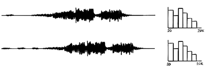
Figure 3.1 Comparison of two audio clips using frequency distribution

Heuristics are context-specific, and a good heuristic can help optimize solutions substantially. The maze scenario from chapter 2 will be adjusted to demonstrate the concept of creating heuristics by introducing an interesting dynamic. Instead of treating all movements the same way and measuring better solutions purely by paths with fewer actions (shallow depth in the tree), movements in different directions now cost different amounts to execute. There’s been some strange shift in the gravity of our maze, and moving north or south now costs five times as much as moving east or west (figure 3.2).

Figure 3.2 Adjustments to the maze example: gravity

In the adjusted maze scenario, the factors influencing the best possible path to the goal are the number of actions taken and the sum of the cost for each action in a respective path.

In figure 3.3, all possible paths in the tree are represented to highlight the options available, indicating the costs of the respective actions. Again, this example demonstrates the search space in the trivial maze scenario and does not often apply to real-life scenarios. The algorithm will be generating the tree as part of the search.

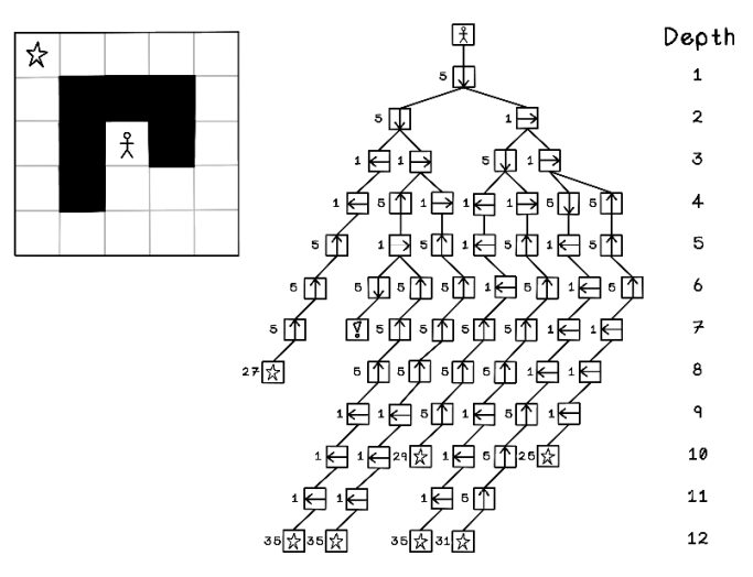
Figure 3.3 All possible movement options represented as a tree

A heuristic for the maze problem can be defined as follows: “Good paths minimize cost of movement and minimize total moves to reach the goal.” This simple heuristic helps guide which nodes are visited because we are applying some domain knowledge to solve the problem.

Thought Experiment: Given the following scenario, what heuristic can you imagine?

Several miners specialize in different types of mining, including diamond, gold, and platinum. All the miners are productive in any mine, but they mine faster in mines that align with their specialties. Several mines that can contain diamonds, gold, and platinum are spread across an area, and depots appear at different distances between mines. If the problem is to distribute miners to maximize their efficiency and reduce travel time, what could a heuristic be?

Thought Experiment: Possible solution

A sensible heuristic would include assigning each miner to a mine of their specialty and tasking them with traveling to the depot closest to that mine. This can also be interpreted as minimizing assigning miners to mines that are not their specialty and minimizing the distance traveled to depots.

Informed search: Looking for solutions with guidance

Informed search, also known as heuristic search, is an algorithm that uses both breadth-first search and depth-first search approaches combined with some intelligence. The search is guided by heuristics, given some predefined knowledge of the problem at hand.

We can employ several informed search algorithms, depending on the nature of the problem, including Greedy Search (also known as Best-first Search). The most popular and useful informed search algorithm, however, is A*.

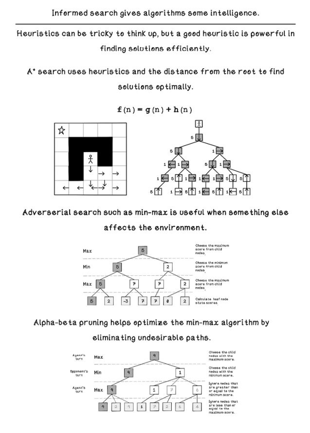
A* search

A* search is pronounced “A star search.” The A* algorithm usually improves performance by estimating heuristics to minimize the cost of the next node visited.

Total cost is calculated with two metrics: the total distance from the start node to the current node and the estimated cost of moving to a specific node by using a heuristic. When we are attempting to minimize cost, a lower value indicates a better-performing solution (figure 3.4).

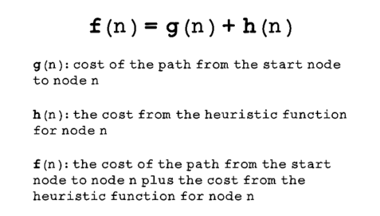
Figure 3.4 The function for the A* search algorithm

The following example of processing is an abstract example of how a tree is visited using heuristics to guide the search. The focus is on the heuristic calculations for the different nodes in the tree.

Breadth-first search visits all nodes on each depth before moving to the next depth. Depth-first search visits all nodes down to the final depth before traversing back to the root and visiting the next path. A* search is different, in that it does not have a predefined pattern to follow; nodes are visited in the order based on their heuristic costs. Note that the algorithm does not know the costs of all nodes up front. Costs are calculated as the tree is explored or generated, and each node visited is added to a stack, which means nodes that cost more than nodes already visited are ignored, saving computation time (figures 3.5, 3.6, and 3.7).

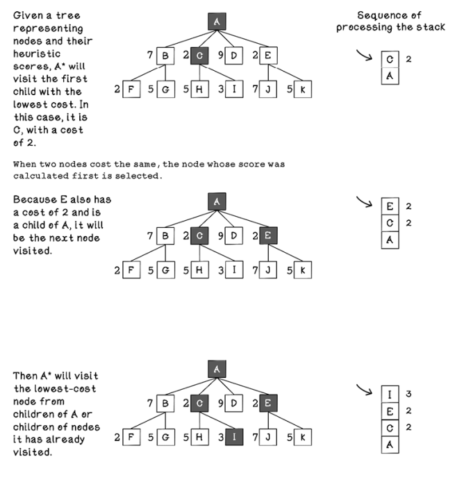
Figure 3.5 The sequence of tree processing using A* search (part 1)

Figure 3.6 The sequence of tree processing using A* search (part 2)

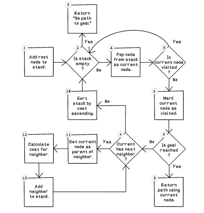
Figure 3.7 Flow for the A* search algorithm

Let’s walk through the flow of the A* search algorithm:

1. Add root node to stack. The A* search algorithm can be implemented with a stack in which the last object added is processed first (last-in, first-out, or LIFO). The first step is adding the root node to the stack.

2. Is stack empty? If the stack is empty, and no path has been returned in step 8 of the algorithm, there is no path to the goal. If there are still nodes in the queue, the algorithm can continue its search.

3. Return No path to goal. This step is the one possible exit from the algorithm if no path to the goal exists.

4. Pop node from stack as current node. By pulling the next object from the stack and setting it as the current node of interest, we can explore its possibilities.

5. Is current node visited? If the current node has not been visited, it hasn’t been explored yet and can be processed now.

6. Mark current node as visited. This step indicates that this node has been visited to prevent unnecessary repeat processing.

7. Is goal reached? This step determines whether the current neighbor contains the goal that the algorithm is searching for.

8. Return path using current node. By referencing the parent of the current node, then the parent of that node, and so on, the path from the goal to the root is described. The root node will be a node without a parent.

9. Current has next neighbor? If the current node has more possible moves to make in the maze example, that move can be added to be processed. Otherwise, the algorithm can jump to step 2, in which the next object in the stack can be processed if it is not empty. The nature of the LIFO stack allows the algorithm to process all nodes to a leaf-node depth before backtracking to visit other children of the root node.

10. Sort stack by cost ascending. When the stack is sorted by the cost of each node in the stack ascending, the lowest-cost node is processed next, allowing the cheapest node always to be visited.

11. Set current node as parent of neighbor. Set the origin node as the parent of the current neighbor. This step is important for tracing the path from the current neighbor to the root node. From a map perspective, the origin is the position that the player moved from, and the current neighbor is the position that the player moved to.

12. Calculate cost for neighbor. The cost function is critical for guiding the A* algorithm. The cost is calculated by summing the distance from the root node with the heuristic score for the next move. More-intelligent heuristics will directly influence the A* algorithm for better performance.

13. Add neighbor to stack. The neighbor node is added to the stack for its children to be explored later. Again, this stacking mechanism allows nodes to be processed to the utmost depth before processing neighbors at shallow depths.

Similar to depth-first search, the order of child nodes influences the path selected, but less drastically. If two nodes have the same cost, the first node is visited before the second (figures 3.8, 3.9, and 3.10).

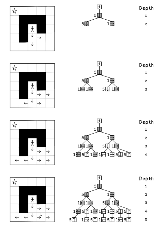
Figure 3.8 The sequence of tree processing using A* search (part 1)

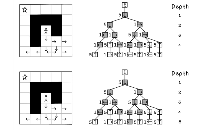
Figure 3.9 The sequence of tree processing using A* search (part 2)

Figure 3.10 Nodes visited in the entire tree after A* search

Notice that there are several paths to the goal, but the A* algorithm finds a path to the goal while minimizing the cost to achieve it, with fewer moves and cheaper move costs based on north and south moves being more expensive.

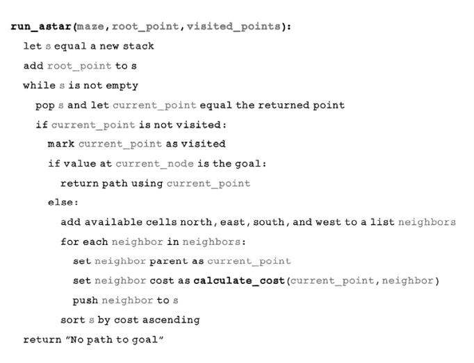
Pseudocode

The A* algorithm uses a similar approach to the depth-first search algorithm but intentionally targets nodes that are cheaper to visit. A stack is used to process the nodes, but the stack is ordered by cost ascending every time a new calculation happens. This order ensures that the object popped from the stack is always the cheapest, because the cheapest is first in the stack after ordering:

The functions for calculating the cost are critical to the operation of A* search. The cost function provides the information for the algorithm to seek the cheapest path. In our adjusted maze example, a higher cost is associated with moving up or down. If there is a problem with the cost function, the algorithm may not work.

The following two functions describe how cost is calculated. The distance from the root node is added to the cost of the next movement. Based on our hypothetical example, the cost of moving north or south influences the total cost of visiting that node:

Uninformed search algorithms such as breadth-first search and depth-first search explore every possibility exhaustively and result in the optimal solution. A* search is a good approach when a sensible heuristic can be created to guide the search. It computes more efficiently than uninformed search algorithms, because it ignores nodes that cost more than nodes already visited. If the heuristic is flawed, however, and doesn’t make sense for the problem and context, poor solutions will be found instead of optimal ones.

Use cases for informed search algorithms

Informed search algorithms are versatile and useful for several real-world use cases in which heuristics can be defined, such as the following:

• Path finding for autonomous game characters in video games—Game developers often use this algorithm to control the movement of enemy units in a game in which the goal is to find the human player within an environment.

• Parsing paragraphs in natural language processing (NLP)—The meaning of a paragraph can be broken into a composition of phrases, which can be broken into a composition of words of different types (like nouns and verbs), creating a tree structure that can be evaluated. Informed search can be useful in extracting meaning.

• Telecommunications network routing—Guided search algorithms can be used to find the shortest paths for network traffic in telecommunications networks to improve performance. Servers/network nodes and connections can be represented as searchable graphs of nodes and edges.

• Single-player games and puzzles—Informed search algorithms can be used to solve single-player games and puzzles such as the Rubik’s Cube, because each move is a decision in a tree of possibilities until the goal state is found.

Adversarial search: Looking for solutions in a changing environment

The search example of the maze game involves a single actor: the player. The environment is affected only by the single player; thus, that player generates all possibilities. The goal until now was to maximize the benefit for the player: choosing paths to the goal with the shortest distance and cost.

Adversarial search is characterized by opposition or conflict. Adversarial problems require us to anticipate, understand, and counteract the actions of the opponent in pursuit of a goal. Examples of adversarial problems include two-player turn-based games such as Tic-Tac-Toe and Connect Four. The players take turns for the opportunity to change the state of the environment of the game to their favor. A set of rules dictates how the environment may be changed and what the winning and end states are.

A simple adversarial problem

This section uses the game of Connect Four to explore adversarial problems. Connect Four (figure 3.11) is a game consisting of a grid in which players take turns dropping tokens into a specific column. The tokens in a specific column pile up, and any player who manages to create four adjacent sequences of their tokens—vertically, horizontally, or diagonally—wins. If the grid is full, with no winner, the game results in a draw.

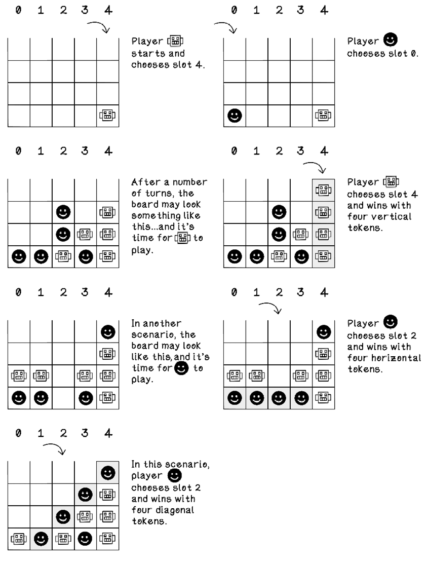
Figure 3.11 The game of Connect Four

Min-max search: Simulate actions and choose the best future

Min-max search aims to build a tree of possible outcomes based on moves that each player could make and favor paths that are advantageous to the agent while avoiding paths that are favorable to the opponent. To do so, this type of search simulates possible moves and scores the state based on a heuristic after making the respective move. Min-max search attempts to discover as many states in the future as possible; but due to memory and computation limitations, discovering the entire game tree may not be realistic, so it searches to a specified depth. Min-max search simulates the turns taken by each player, so the depth specified is directly linked to the number of turns between both players. A depth of 4, for example, means that each player has had 2 turns. Player A makes a move, player B makes a move, player A makes another move, and Player B makes another move.

Heuristics

The min-max algorithm uses a heuristic score to make decisions. This score is defined by a crafted heuristic and is not learned by the algorithm. If we have a specific game state, every possible valid outcome of a move from that state will be a child node in the game tree.

Assume that we have a heuristic that provides a score in which positive numbers are better than negative numbers. By simulating every possible valid move, the min-max search algorithm tries to minimize making moves where the opponent will have an advantage or a winning state and maximize making moves that give the agent an advantage or a winning state.

Figure 3.12 illustrates a min-max search tree. In this figure, the leaf nodes are the only nodes where the heuristic score is calculated, since these states indicate a winner or a draw. The other nodes in the tree indicate states that are in progress. Starting at the depth where the heuristic is calculated and moving upward, either the child with the minimum score or the child with the maximum score is chosen, depending on whose turn is next in the future simulated states. Starting at the top, the agent attempts to maximize its score; and after each alternating turn, the intention changes, because the aim is to maximize the score for the agent and minimize the score for the opponent.

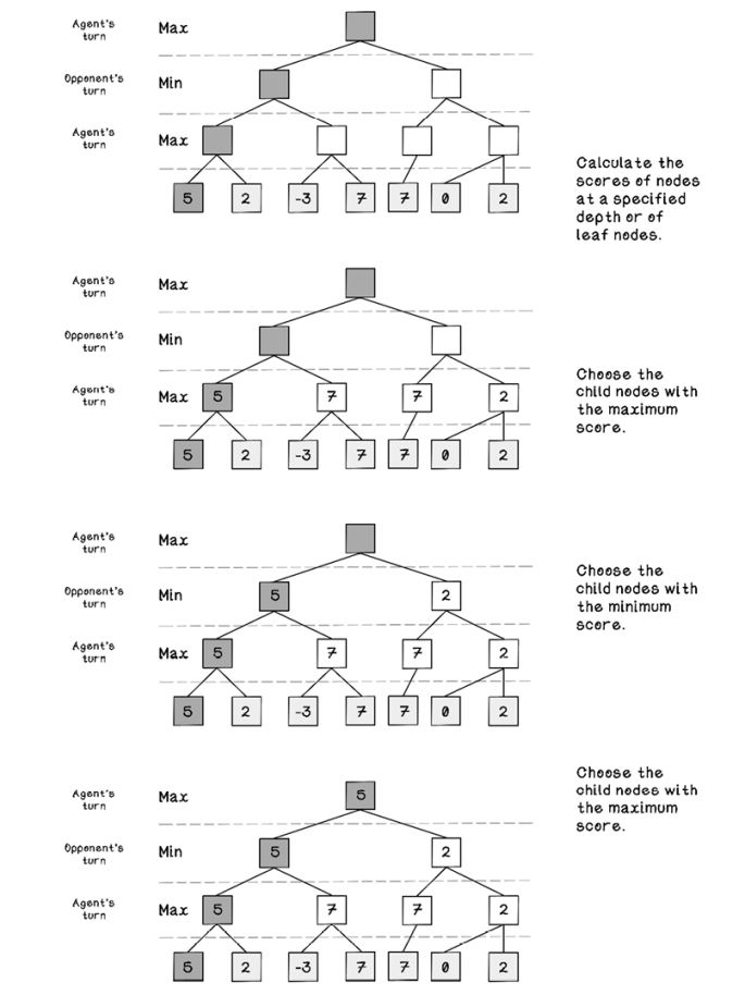
Figure 3.12 The sequence of tree processing using min-max search

Exercise: What values would propagate in the following Min-max tree?

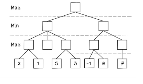
Solution: What values would propagate in the following Min-max tree?

Because the min-max search algorithm simulates possible outcomes, in games that offer a multitude of choices, the game tree explodes, and it quickly becomes too computationally expensive to explore the entire tree. In the simple example of Connect Four played on a 5 × 4 block board, the number of possibilities already makes exploring the entire game tree on every turn inefficient (figure 3.13).

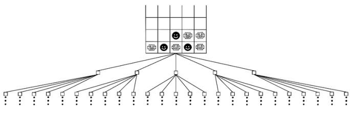
Figure 3.13 The explosion of possibilities while searching the game tree

To use min-max search in the Connect Four example, the algorithm essentially makes all possible moves from a current game state; then it determines all possible moves from each of those states until it finds the path that is most favorable. Game states that result in a win for the agent return a score of 10, and states that result in a win for the opponent return a score of -10. Min-max search tries to maximize the positive score for the agent (figures 3.14 and 3.15).

Figure 3.14 Scoring for the agent versus scoring for the opponent

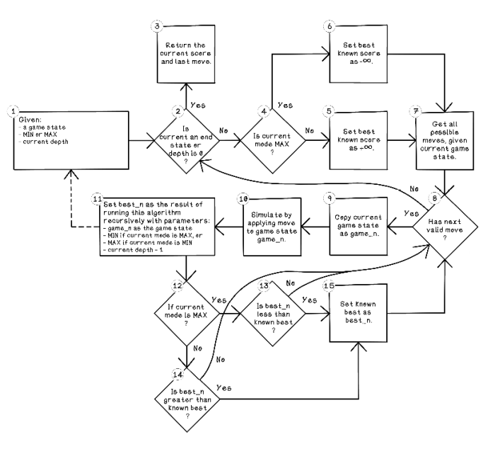
Figure 3.15 Flow for the min-max search algorithm

Although the flow chart for the min-max search algorithm looks complex due to its size, it really isn’t. The number of conditions that check whether the current state is to maximize or minimize causes the chart to bloat.

Let’s walk through the flow of the min-max search algorithm:

1. Given a game state, whether the current mode is minimization or maximization, and a current depth, the algorithm can start. It is important to understand the inputs for the algorithm, as the min-max search algorithm is recursive. A recursive algorithm calls itself in one or more of its steps. It is important for a recursive algorithm to have an exit condition to prevent it from calling itself forever.

2. Is current an end state or depth is 0? This condition determines whether the current state of the game is a terminal state or whether the desired depth has been reached. A terminal state is one in which one of the players has won or the game is a draw. A score of 10 represents a win for the agent, and a score of -10 represents a win for the opponent, and a score of 0 indicates a draw. A depth is specified, because traversing the entire tree of possibilities to all end states is computationally expensive and will likely take too long on the average computer. By specifying a depth, the algorithm can look a few turns into the future to determine whether a terminal state exists.

3. Return the current score and last move. The score for the current state is returned if the current state is a terminal game state or if the specified depth has been reached.

4. Is current mode MAX? If the current iteration of the algorithm is in the maximize state, it tries to maximize the score for the agent.

5. Set best known score as +∞. If the current mode is to minimize the score, the best score is set to positive infinity, because we know that the scores returned by the game states will always be less. In actual implementation, a really large number is used rather than infinity.

6. Set best known score as -∞. If the current mode is to maximize the score, the best score is set to negative infinity, because we know that the scores returned by the game states will always be more. In actual implementation, a really large negative number is used rather than infinity.

7. Get all possible moves, given current game state. This step specifies a list of possible moves that can be made, given the current game state. As the game progresses, not all moves available at the start may be available anymore. In the Connect Four example, a column may be filled; therefore, a move selecting that column is invalid.

8. Has next valid move? If any possible moves have not been simulated yet and there are no more valid moves to make, the algorithm short-circuits to returning the best move in that instance of the function call.

9. Copy current game state as game_n. A copy of the current game state is required to perform simulations of possible future moves on it.

10. Simulate by applying move to game state game_n. This step applies the current move of interest to the copied game state.

11. Set best_n as the result of running this algorithm recursively. Here’s where recursion comes into play. best_n is a variable used to store the next best move, and we’re making the algorithm explore future possibilities from this move.

12. If current mode is MAX? When the recursive call returns a best candidate, this condition determines whether the current mode is to maximize the score.

13. Is best_n less than known best? This step determines whether the algorithm has found a better score than one previously found if the mode is to maximize the score.

14. Is best_n greater than known best? This step determines whether the algorithm has found a better score than one previously found if the mode is to minimize the score.

15. Set known best as best_n. If the new best score is found, set the known best as that score.

    Given the Connect Four example at a specific state, the min-max search algorithm generates the tree shown in figure 3.16. From the start state, every possible move is explored. Then each move from that state is explored until a terminal state is found—either the board is full or a player has won.

    

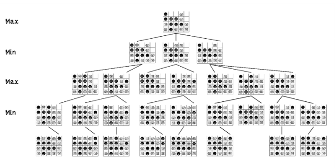
    Figure 3.16 A representation of the possible states in a Connect Four game

    The highlighted nodes in figure 3.17 are terminal state nodes in which draws are scored as 0, losses are scored as -10, and wins are scored as 10. Because the algorithm aims to maximize its score, a positive number is required, whereas opponent wins are scored with a negative number.

    

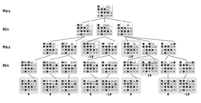
    Figure 3.17 The possible end states in a Connect Four game

    When these scores are known, the min-max algorithm starts at the lowest depth and chooses the node whose score is the minimum value (figure 3.18).

    

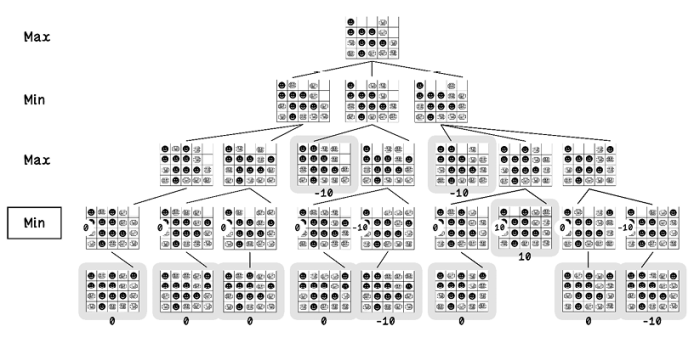
    Figure 3.18 The possible scores for end states in a Connect Four game (part 1)

    Then, at the next depth, the algorithm chooses the node whose score is the maximum value (figure 3.19).

    

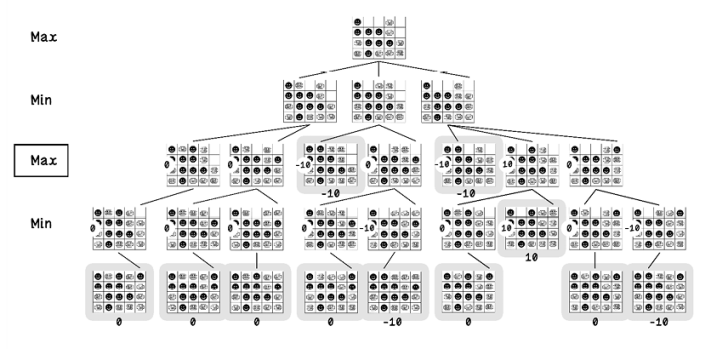
    Figure 3.19 The possible scores for end states in a Connect Four game (part 2)

    Finally, at the next depth, nodes whose score is the minimum are chosen, and the root node chooses the maximum of the options. By following the nodes and score selected and intuitively applying ourselves to the problem, we see that the algorithm selects a path to a draw to avoid a loss. If the algorithm selects the path to the win, there is a high likelihood of a loss in the next turn. The algorithm assumes that the opponent will always make the smartest move to maximize their chance of winning (figure 3.20).

    

    Figure 3.20 The possible scores for end states in a Connect Four game (part 3)

    The simplified tree in figure 3.21 represents the outcome of the min-max search algorithm for the given game state example.

    

    Figure 3.21 Simplified game tree with min-max scoring

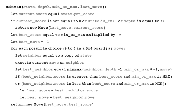
    Pseudocode

    The min-max search algorithm is implemented to be a recursive function. The function is provided with the current state, desired depth to search, minimization or maximization mode, and last move. The algorithm terminates by returning the best move and score for every child at every depth in the tree. Comparing the code with the flow chart in figure 3.15, we notice that the tedious conditions of checking whether the current mode is maximizing or minimizing are not as apparent. In the pseudocode, 1 or -1 represents the intention to maximize or minimize, respectively. By using some clever logic, the best score, conditions, and switching states can be done via the principle of negative multiplication, in which a negative number multiplied by another negative number results in a positive. So if -1 indicates the opponent’s turn, multiplying it by -1 results in 1, which indicates the agent’s turn. Then, for the next turn, 1 multiplied by -1 results in -1 to indicate the opponent’s turn again:

    

    Alpha-beta pruning: Optimize by exploring the sensible paths only

    Alpha-beta pruning is a technique used with the min-max search algorithm to short-circuit exploring areas of the game tree that are known to produce poor solutions. This technique optimizes the min-max search algorithm to save computation, because insignificant paths are ignored. Because we know how the Connect Four example game tree explodes, we clearly see that ignoring more paths will improve performance significantly (figure 3.22).

    

    Figure 3.22 An example of alpha-beta pruning

    The alpha-beta pruning algorithm works by storing the best score for the maximizing player and the best score for the minimizing player as alpha and beta, respectively. Initially, alpha is set as -∞, and beta is set as ∞—the worst score for each player. If the best score of the minimizing player is less than the best score of the maximizing player, it is logical that other child paths of the nodes already visited would not affect the best score.

    Figure 3.23 illustrates the changes made in the min-max search flow to accommodate the optimization of alpha-beta pruning. The highlighted blocks are the additional steps in the min-max search algorithm flow.

    

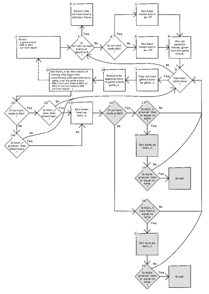
    Figure 3.23 Flow for the min-max search algorithm with alpha-beta pruning

    The following steps are additions to the min-max search algorithm. These conditions allow termination of exploration of paths when the best score found will not change the outcome:

16. Is current mode MAX? Again, determine whether the algorithm is currently attempting to maximize or minimize the score.

17. Is best_n greater than or equal to alpha? If the current mode is to maximize the score and the current best score is greater than or equal to alpha, no better scores are contained in that node’s children, allowing the algorithm to ignore that node.

18. Set alpha as best_n. Set the variable alpha as best_n.

19. Is alpha greater than or equal to beta? The score is as good as other scores found, and the rest of the exploration of that node can be ignored by breaking.

20. Is best_n less than or equal to beta? If the current mode is to minimize the score and the current best score is less than or equal to beta, no better scores are contained in that node’s children, allowing the algorithm to ignore that node.

21. Set beta as best_n. Set the variable beta as best_n.

22. Is alpha greater than or equal to beta? The score is as good as other scores found, and the rest of the exploration of that node can be ignored by breaking.

Pseudocode

The pseudocode for achieving alpha-beta pruning is largely the same as the code for min-max search, with the addition of keeping track of the alpha and beta values and maintaining those values as the tree is traversed. Note that when minimum(min) is selected the variable min_or_max is -1, and when maximum(max) is selected, the variable min_or_max is 1:

Use cases for adversarial search algorithms

Informed search algorithms are versatile and useful in real-world use cases such as the following:

• Creating game-playing agents for turn-based games with perfect information—In some games, two or more players act on the same environment. There have been successful implementations of chess, checkers, and other classic games. Games with perfect information are games that do not have hidden information or random chance involved.

• Creating game-playing agents for turn-based games with imperfect information—Unknown future options exist in these games, including games like poker and Scrabble.

• Adversarial search and ant colony optimization (ACO) for route optimization—Adversarial search is used in combination with the ACO algorithm (discussed in chapter 6) to optimize package-delivery routes in cities.

Summary of Intelligent search