Human capital development before age five*
Janet Currie and Douglas Almond, Columbia University, [email protected]
Abstract
This chapter seeks to set out what economists have learned about the effects of early childhood influences on later life outcomes, and about ameliorating the effects of negative influences. We begin with a brief overview of the theory which illustrates that evidence of a causal relationship between a shock in early childhood and a future outcome says little about whether the relationship in question is biological or immutable. We then survey recent work which shows that events before five years old can have large long term impacts on adult outcomes. Child and family characteristics measured at school entry do as much to explain future outcomes as factors that labor economists have more traditionally focused on, such as years of education. Yet while children can be permanently damaged at this age, an important message is that the damage can often be remediated. We provide a brief overview of evidence regarding the effectiveness of different types of policies to provide remediation. We conclude with a list of some of the many outstanding questions for future research.
Keywords
Human capital; Early childhood; Health; Fetal origins
1 Introduction
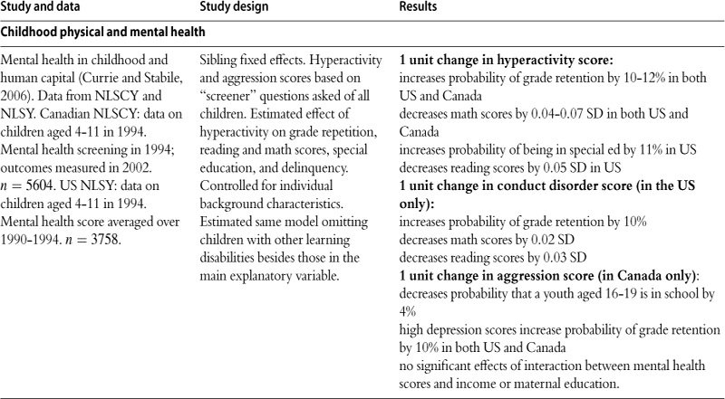
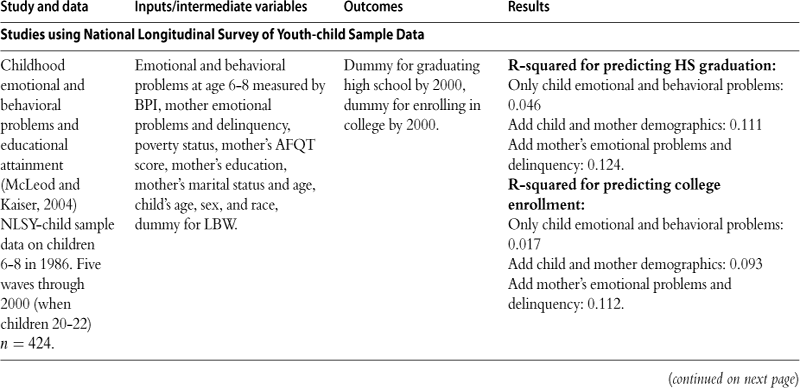
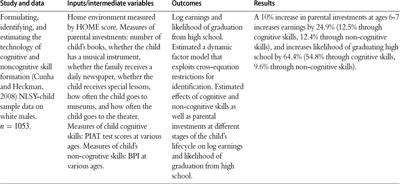
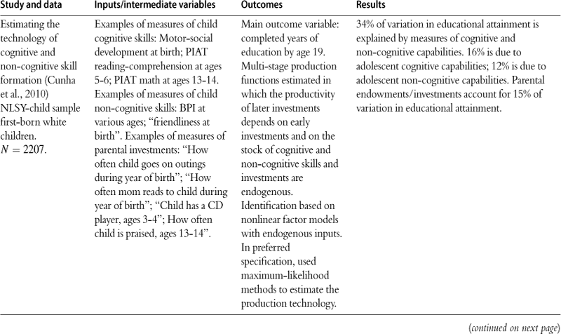
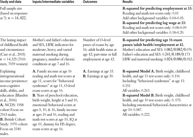
The last decade has seen a blossoming of research on the long term effects of early childhood conditions across a range of disciplines. In economics, the focus is on how human capital accumulation responds to the early childhood environment. In 2000, there were no articles on this topic in the Journal of Political Economy, Quarterly Journal of Economics, or the American Economic Review (excluding the Papers and Proceedings), but there have been five or six per year in these journals since 2005. This work has been spurred by a growing realization that early life conditions can have persistent and profound impacts on later life. Table 1 summarizes several longitudinal studies which suggest that characteristics that are measured as of age 7 can explain a great deal of the variation in educational attainment, earnings as of the early 30s, and the probability of employment. For example, McLeod and Kaiser (2004) use data from the National Longitudinal Surveys and find that children’s test scores and background variables measured as of ages 6 to 8 predict about 12% of the variation in the probability of high school completion and about 11% of the variation in the probability of college completion. Currie and Thomas (1999b) use data from the 1958 British Birth Cohort study and find that 4% to 5% of the variation in employment at age 33 can be predicted, and as much as 20% of the variation in wages. Cunha and Heckman (2008) and Cunha et al. (2010) estimate structural models in which initial endowments and investments feed through to later outcomes; they arrive at estimates that are of a similar order of magnitude for education and wages. To put these results in context, labor economists generally feel that they are doing well if they can explain 30% of the variation in wages in a human capital earnings function.
Table 1
How much of the differences in later outcomes (test scores, educational attainment, earnings) can be explained by early childhood factors?

This chapter seeks to set out what economists have learned about the importance of early childhood influences on later life outcomes, and about ameliorating the effects of negative influences. We begin with a brief overview of the theory which illustrates that evidence of a causal relationship between a shock in early childhood and a future outcome says little about whether the relationship in question is biological or immutable. Parental and social responses are likely to be extremely important in either magnifying or mitigating the effects of a shock. Given that this is the case, it can sometimes be difficult to interpret the wealth of empirical evidence that is accumulating in terms of an underlying structural framework.
The theoretical framework is laid out in Section 2 and followed by a brief discussion of methods in Section 3. We do not attempt to cover issues such as identification and instrumental variables methods, which are covered in some depth elsewhere (cf Angrist and Pischke (2009)). Instead, we focus on several issues that come up frequently in the early influences literature, including estimation using small samples and the potentially high return to better data.
Section 4 discusses the evidence for long-term effects of early life influences in greater detail, while Section 5 focuses on the evidence regarding remediation programs. The discussion of early life influences is divided into two subsections corresponding to in utero influences and after birth influences. The discussion of remediation programs starts from the most general sort of program, income transfers, and goes on to discuss interventions that are increasingly targeted at specific domains. In surveying the evidence we have attempted to focus on recent papers, and especially those that propose a plausible strategy for identifying causal effects. We have focused on papers that emphasize early childhood, but in instances in which only evidence regarding effects on older children is available, we have sometimes strayed from this rule. A summary of most of the papers discussed in these sections is presented in Tables 4 through 13. A list of acronyms used in the tables appears in Appendix A. We conclude with a summary and a discussion of outstanding questions for future research in Section 6.
2 Conceptual framework
Grossman (1972) models health as a stock variable that varies over time in response to investments and depreciation. Because some positive portion of the previous period’s health stock vanishes in each period (e.g., age in years), the effect of the health stock and health investments further removed in time from the current period tends to fade out. As individuals age, the early childhood health stock and the prior health investments that it embodies become progressively less important.
In contrast, the “early influences” literature asks whether health and investments in early childhood have sustained effects on adult outcomes. The magnitude of these effects may persist or even increase as individuals age because childhood development occurs in distinct stages that are more or less influential of adult outcomes.
Defining h as health or human capital at the completion of childhood, we can retain the linearity of h in investments and the prior health stock as in Grossman (1972), but leave open whether there is indeed “fade out” (i.e. depreciation). For simplicity, we will consider a simple two-period childhood.1 We can consider production of h:
![]() (1)
(1)
where:
![]()
For a given level of total investments I1 + I2, the allocation of investments between period 1 and 2 will affect h for γ = 0.5. If γ > 0.5, then health at the end of period 1 is more important to h than investments in the second period, and if γ A > 1, h may respond more than one-for-one with I1. Thus, (1) admits the possibility that certain childhood periods may exert a disproportionate effect on adult outcomes that does not necessarily decline monotonically with age. This functional form says more than “early life” matters; it suggests that early-childhood events may be more influential than later childhood events.
2.1 Complementarity
The assumption that inputs at different stages of childhood have linear effects is common in economics. While it opens the door to “early origins,” perfect substitutability between first and second period investments in (1) is a strong assumption. The absence of complementarity implies that all investments should be concentrated in one period (up to a discount factor) and no investments should be made during the low-return period. In addition, with basic preference assumptions, perfect substitutability “hardwires” the optimal investment response to early-life shocks to be compensatory, as seen in Section 2.3.
As suggested by Heckman (2007), a more flexible “developmental” technology is the constant elasticity of substitution (CES) function:
![]() (2)
(2)
For a given total investment level I1 +I2, how the allocation between period 1 and 2 will also affect h depends on the elasticity of substitution, 1/(1 – ϕ), and the share parameter, γ. For ϕ = 1 (perfect substitutability of investments), (2) reduces to (1).
Heckman (2007) highlights two features of “capacity formation” beyond those captured in (2). First, there may be “dynamic complementarities” which imply that investments in period t are more productive when there is a high level of capability in period t – 1. For example, if the factor productivity term A in (2) were an increasing function of h0, the health endowment immediately prior to period 1, this would raise the return to investments during childhood. Second, there may be “self-productivity” which implies that higher levels of capacity in one period create higher levels of capacity in future periods. This feature is especially noteworthy when h is multidimensional, as it would imply that “cross-effects” are positive, e.g. health in period 1 leads to higher cognitive ability in period 2. “Self-productivity” is more trivial in the unidimensional case like Grossman (1972)—even though the effect of earlier health stocks tends to fade out as the time passes, there is still memory as long as depreciation in each period is less than total (i.e., when δ < in Zweifel et al. (2009)).
Here, we will use the basic framework in (2) to consider the effect of exogenous shocks μg to health investments that occur during the first childhood period.2 We begin with the simplest case, where investments do not respond to μg (and denote these investments ![]() and
and ![]() ). Net investments in the first period are:
). Net investments in the first period are:
![]()
We assume that μg is independent of ![]() . While μg can be positive or negative, we assume
. While μg can be positive or negative, we assume ![]() + μg > 0. We will then relax the assumption of fixed investments, and consider endogenous responses to investments in the second period, i.e.
+ μg > 0. We will then relax the assumption of fixed investments, and consider endogenous responses to investments in the second period, i.e. ![]() , and how this investment response may mediate the observed effect on h.
, and how this investment response may mediate the observed effect on h.
2.2 Fixed investments
Conceptually, we can trace out the effect of μg while holding other inputs fixed, i.e., we assume no investment response to this shock in either period. Albeit implicitly, most biomedical and epidemiological studies in the “early origins” literature aim to inform us about this ceteris paribus, “biological” relationship.
In this two-period CES production function adopted from Heckman (2007), the impact of an early-life shock on adult outcomes is:
![]() (3)
(3)
The simplest production technology is the perfect substitutability case where ϕ = 1. In this case:
![]()
Damage to adult human capital is proportional to the share parameter on period 1 investments, and is unrelated to the investment level ![]() .
.
For less than perfect substitutability between periods, there is diminishing marginal productivity of the investment inputs. Thus, shocks experienced at different baseline investment levels have heterogenous effects on h. Other things equal, those with higher baseline levels of investment will experience more muted effects in h than those where baseline investment is low. A recurring empirical finding is that long-term damage due to shocks is more likely among poorer families (Currie and Hyson, 1999). This is in part due to the fact that children in poorer families are subject to more or larger early-life shocks (Case et al., 2002; Currie and Stabile, 2003). However, it is also possible that the same shock will have a greater impact among children in poorer families if these children have lower period t investment levels to begin with. This occurs because they are on a steeper portion of the production function. Ceteris paribus, this would tend to accentuate the effect of an equivalent-sized μg shock on h among poor families.3,4
2.2.1 Remediation
Is it possible to alter “bad” early trajectories? In other words, what is the effect of a shock μ′g > 0 experienced during the second period on h? Remediation is of interest to the extent that (3) is substantially less than zero. However, large damage to h from μg per se says little about the potential effectiveness of remediation in the second period, as both initial damage and remediation are distinct functions of the three parameters A, γ, and ϕ.
The effectiveness of remediation relative to initial damage is:
![]() (4)
(4)
Thus, for ![]() >
> ![]() and a given value of γ, a unit of remediation will be more effective at low elasticities of substitution—the lack of
and a given value of γ, a unit of remediation will be more effective at low elasticities of substitution—the lack of ![]() was the more critical shortfall prior to the shock. If
was the more critical shortfall prior to the shock. If ![]() <
< ![]() high elasticities of substitution increase the effectiveness of remediation—adding to the existing abundance of
high elasticities of substitution increase the effectiveness of remediation—adding to the existing abundance of ![]() remains effective.
remains effective.
Fortunately, it is not necessary to observe investments and estimate all three parameters in order to assess the scope for remediation. In some cases, we merely need to observe how a shock in the second period, μ′g, affects h. Furthermore, this does not necessarily require a distinct shock in addition to μg. In an overlapping generations framework, the same shock, μg = μ′g could affect one cohort in the first childhood period (but not the second) and an older cohort in the second period (but not the first). For a small, “double-barreled” shock, we would have reduced form estimates of both the damage in (3) and the potential to alter trajectories in (4).5 For example, in addition to observing how income during the prenatal period affects newborn health (Kehrer and Wolin, 1979), we might also be able to see how parental income affects the health of preschool age children to gain a sense of what opportunities there are to remediate negative income shocks experienced during pregnancy.
2.3 Responsive investments
Most analyses of “early origins” focus on estimating the reduced form effect, δh/δμg. Whether this empirical relationship represents a purely biological effect or also includes the effect of responsive investments is an open question. In general, to the extent that “early origins” are important, so too will be any response of childhood investments to μg. For expositional purposes, we will consider μg < 0 and responses that either magnify or attenuate initial damage.
Unless the investment response is costless, damage estimates that monetize δh/δμg alone will tend to understate total damage. In the extreme, investment responses could fully offset the effect of early-life shocks on h, but this would not mean that such shocks were costless (Deschnes and Greenstone, 2007). More generally, the damage from early-life shocks will be understated if we focus only on long-term effects and there are compensatory investments (i.e. investments that are negatively correlated with the early-life shock ![]() ). The cost of investments that help remediate damage should be included. But even when the response is reinforcing
). The cost of investments that help remediate damage should be included. But even when the response is reinforcing ![]() , total costs can still be understated by focussing on the reduced form damage to h alone (see below).
, total costs can still be understated by focussing on the reduced form damage to h alone (see below).
To consider correlated investment responses more formally, we assume parents observe μg at the end of the first period. The direction of the investment response— whether reinforcing or compensatory—will be shaped by how substitutable period 2 investments are for those in period 1. If substitutability is high, the optimal response will tend to be compensatory, and thereby help offset damage to h.
A compensatory response is readily seen in the case of perfect substitutability. Cunha and Heckman (2007) observed that economic models commonly assume that production at different stages of childhood are perfect substitutes. When ϕ = 1, (2) reduces to:
![]() (5)
(5)
This linear production technology is akin to that used in a previous Handbook chapter on intergenerational mobility (Solon, 1999), which likewise considered parental investments in children’s human capital. Further, Solon (1999) assumed parent’s utility trades off own consumption against the child’s human capital:
![]() (6)
(6)
where p denotes parents and C their consumption. The budget constraint is:
![]() (7)
(7)
With standard preferences, changes to h through μg will “unbalance” the marginal utilities in h versus C.6 If μg is negative, the marginal utility of h becomes too high relative to that in consumption. The technology in (5) permits parents to convert some consumption into h at a constant rate. This will cause ![]() to increase, which attenuates the effect of the μg damage. This attenuation comes at the cost of reduced parental utility. Similarly, if μg is positive parents will “spend the bounty” (at least in part), reduce
to increase, which attenuates the effect of the μg damage. This attenuation comes at the cost of reduced parental utility. Similarly, if μg is positive parents will “spend the bounty” (at least in part), reduce ![]() and increase consumption. Again, this will temper effects on h, leading to an understatement of biological effects in analyses that ignore investments (or parental utility). In either case, perfect substitutability hard-wires the response to be compensatory.
and increase consumption. Again, this will temper effects on h, leading to an understatement of biological effects in analyses that ignore investments (or parental utility). In either case, perfect substitutability hard-wires the response to be compensatory.
The polar opposite technology is perfect complementarity between childhood stages, i.e., a Leontieffproduction function. Here, a compensatory strategy would be completely ineffective in mitigating changes to h. As h is determined by the minimum of period 1 and period 2 investments, optimal period 2 investments should reinforce μg. If μg is negative, parents would seek to reduce I2 and consume more. Despite higher consumption, parents’ utility is reduced on net due to the shock (or this bundle of lower h and higher C would have been selected absent μg). Again, the full-cost of a negative μg shock is understated when parental utility is ignored.
The crossover between reinforcing and compensating responses of ![]() will occur at an intermediate parameter value of substitutability. (The fixed investments case of Section 2.2 can be seen to reflect an optimized response at this point of balance between reinforcing and compensating responses). The value of ϕ at this point of balance will depend on the functional form of parental preferences in (6), as shown for CES utility in Appendix B.
will occur at an intermediate parameter value of substitutability. (The fixed investments case of Section 2.2 can be seen to reflect an optimized response at this point of balance between reinforcing and compensating responses). The value of ϕ at this point of balance will depend on the functional form of parental preferences in (6), as shown for CES utility in Appendix B.
To take a familiar example, assume a Cobb-Douglas utility function of the form:
![]() (8)
(8)
If the production technology is also Cobb-Douglas (ϕ = 0), then no change to ![]() is warranted. If instead substitution between period 1 and period 2 is relatively easy (ϕ > 0), compensating for the shock is optimal. If substitution is relatively difficult (ϕ < 0), then parents should “go with the flow” and reinforce. For this reason, whether conventional reduced form analyses under or over-state “biological” effects (effects with I2 held fixed) depends on how easy it is to substitute the timing of investments across childhood. If the elasticity of substitution across periods is low, then it may be optimal for parents to reinforce the effect of a shock.
is warranted. If instead substitution between period 1 and period 2 is relatively easy (ϕ > 0), compensating for the shock is optimal. If substitution is relatively difficult (ϕ < 0), then parents should “go with the flow” and reinforce. For this reason, whether conventional reduced form analyses under or over-state “biological” effects (effects with I2 held fixed) depends on how easy it is to substitute the timing of investments across childhood. If the elasticity of substitution across periods is low, then it may be optimal for parents to reinforce the effect of a shock.
Tension between preferences and the production technology may also be relevant for within-family investment decisions. For example, Behrman et al. (1982) considered parental preferences that parameterize varying degrees of “inequality aversion” among (multiple) children. Depending on the strength of parents’ inequality aversion relative to the production technology (as reflected by ϕ), parents may reinforce or compensate exogenous within-family differences in early-life health and human capital. If substitutability between periods of childhood is sufficiently difficult (low ϕ), reinforcement of sibling differences will be optimal. This reinforcement may be optimal even when the parents place a higher weight in their utility function on the accumulation of human capital by the less able sibling (see Appendix C). Thus, empirical evidence that some parents reinforce early-life shocks could reveal less about “human nature” than it would reveal about the developmental nature of the childhood production technology.
3 Methods
As discussed above, we confine our discussion to methodological issues that seem particularly germane to the early influences literature. One of these is the question of when sibling fixed effects (or maternal fixed effects) estimation is appropriate. Fixed effects can be a powerful way to eliminate confounding from shared family background characteristics, even when these are not fully observed. This approach is particularly effective when the direction of unobserved sibling-specific confounders can be signed. For example, Currie and Thomas (1995) find that in the cross-section, children who were in Head Start do worse than children who were not. However, compared to their own siblings, Head Start children do better. Since there is little evidence that Head Start children are “favored” by parents or otherwise (on the contrary, in families where one child attends and the other does not, children who attended were more likely to have spent their preschool years in poverty), these contrasting results suggest that unobserved family characteristics are correlated both with Head Start attendance and poor child outcomes. When the effect of such characteristics is accounted for, the positive effects of Head Start are apparent.
However, fixed effects can not control for sibling-specific factors. The theory discussed above suggests that it may be optimal for parents to either reinforce or compensate for the effects of early shocks by altering their own investment behaviors. Whether parents do or do not reinforce/compensate obviously has implications for the interpretation of models estimated using family fixed effects. If on average, families compensate, then fixed effects estimates will understate the total effect of the shock (when the compensation behavior is unobserved or otherwise not accounted for). In some circumstances, such a bias might be benign in the sense that any significant coefficient could then be interpreted as a lower bound on the total effect. It is likely to be more problematic if parents systematically reinforce shocks, because then any effect that is observed results from a combination of underlying effects and parental reactions rather than the shock itself. In the extreme, if parents seized on a characteristic that was unrelated to ability and systematically favored children who had that characteristic, then researchers might wrongly conclude that the characteristic was in fact linked to success even in the absence of parental responses.
The issue of how parents allocate resources between siblings has received a good deal of attention in economics, starting with Becker and Tomes (1976) and Behrman et al. (1982). Some empirical studies from developing countries find evidence of reinforcing behavior (see Rosenzweig and Paul Schultz (1982), Rosenzweig and Wolpin (1988) and Pitt et al. (1990)). Empirical tests of these theories in developed countries such as the United States and Britain generally use adult outcomes such as completed education as a proxy for parental investments (see for example, Griliches (1979), Behrman et al. (1994) and Ashenfelter and Rouse (1998)).
Several recent studies have used birth weight as a measure of the child’s endowment and asked whether explicit measures of parental investments during early childhood are related to birth weight. For example, Datar et al. (2010) use data from the National Longitudinal Survey of Youth-Child and show that low birth weight children are less likely to be breastfed, have fewer well-baby visits, are less likely to be immunized, and are less likely to attend preschool than normal birth weight siblings. However, all of these differences could be due to poorer health among the low birth weight children. For example, if a child is receiving many visits for sick care, they may receive fewer visits for well care and this will not say anything about parental investment behaviors. Hence, Datar et al. (2010) also look at how the presence of low birth weight siblings in the household affects the investments received by normal birth weight children. They find no effect of having a low birth weight sibling on breastfeeding, immunizations, or preschool. The only statistically significant interaction is for well-baby care. This could however, be due to transactions costs. It may be the case that if the low birth weight sibling is getting a lot of medical care, it is less costly to bring the normal birth weight child in for care as well, for example.
Del Bono et al. (2008) estimate a model that allows endowments of other children to affect parental investments in the index child. They find, however, that the results from this dynamic model are remarkably similar to those of mother fixed effects models in most cases. Moreover, although they find a positive effect of birth weight on breastfeeding, the effect is very small in magnitude.
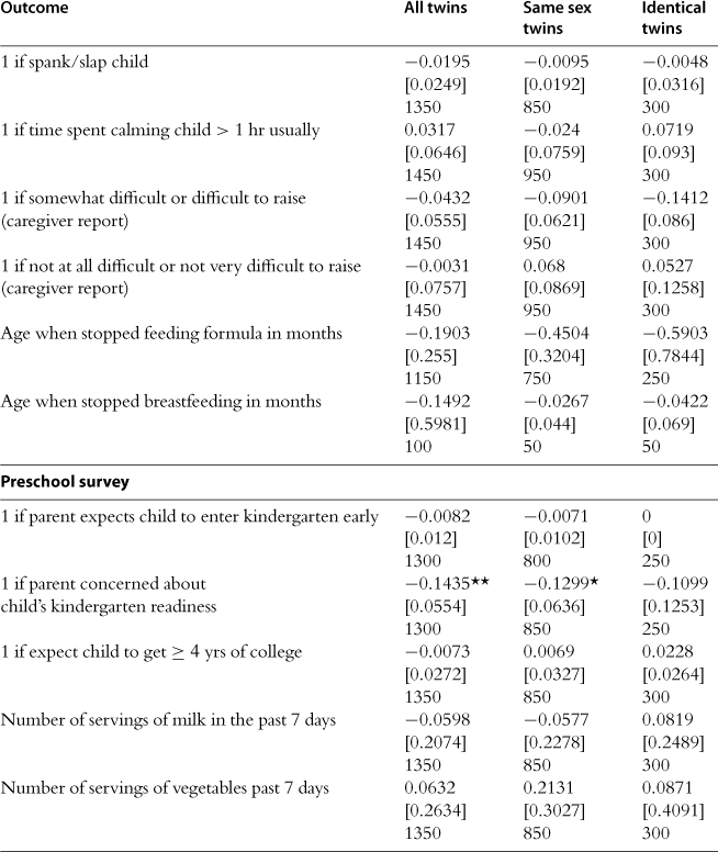
We conducted our own investigation of this issue using data on twins from the Early Childhood Longitudinal Study-Birth Cohort (ECLS-B), using twin differences to control for potential confounders. At the same time, twins routinely have large differences in endowment in the form of birth weight. Table 2 presents estimates for all twins (with and without controls for gender), same sex twins, and identical twins. Overall, there are very few significant differences in the treatment of these twins: Parents seemed to be more concerned about whether the low birth weight twin was ready for school, and to delay introducing solid food (but this is only significant in the identical twin pairs). We see no evidence that parents are more likely to praise, caress, spank or otherwise treat children differently, and despite their worries about school readiness, parents have similar expectations regarding college for both twins. This table largely replicates the basic finding of Royer (2009), who also considered parental investments and birth weight differences in the ECLS-B data. In particular, Royer (2009) focussed on investments soon after birth, finding that breastfeeding, NICU admission, and other measures of neonatal medical care did not vary with within twin pair birth weight differences.
Table 2
Estimated effect of birth weight on parental investments within twin pairs, estimates from the early childhood longitudinal study.
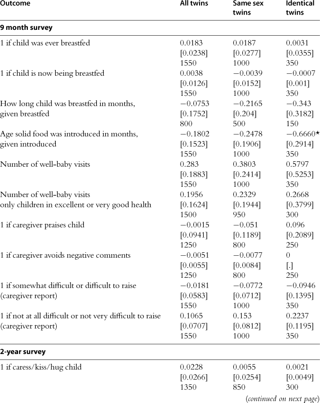
Standard errors clustered on the mother are shown in brackets with sample sizes below. Twin pairs in which a child had a congenital anomaly are omitted. Birth weight measured in kilograms. Each entry is from a separate regression of the dependent variable on birth weight and a mother fixed effect. Models in column 1 also control for child gender. Sample sizes are rounded to the nearest multiple of 50. Significance levels: *** p < 0.001
The parental investment response has also been explored in the context of natural experiments. Kelly (2009) asked whether observed parental investments (e.g., time spent reading to child) were related to flu-induced damages to test scores in the 1958 British birth cohort study but did not detect an investment response.
In an interesting contribution to this literature, Hsin (2009) looks at the relationship between children’s endowments, measured using birth weight, and maternal time use using data from the Child Supplement of the Panel Study of Income Dynamics. She finds that overall, there is little relationship between low birth weight and maternal time investments. However, she argues that this masks important differences by maternal socioeconomic status. In particular, she finds that in models with maternal fixed effects, less educated women spend less time with their low birth weight children, while more educated women spend more time. This finding is based on only 65 sibling pairs who had differences in the incidence of low birth weight, and so requires some corroboration. Still, one interpretation of this result in the context of the Section 2 framework is that the elasticity of substitution between C and h varies by socioeconomic status. In particular, if ψpoor > ψrich, low income parents tend to view their consumption and children’s h as relatively good substitutes. This would lead low-income parents to be more likely to reinforce a negative shock than high-income parents (assuming that the developmental technology, captured by γ and ϕ, does not vary by socioeconomic status). A second possible interpretation of the finding is that parents’ responses may reflect their budget constraint more than their preferences. If parents would like to invest in both children, but have only enough resources to invest adequately in one, then they may be forced to choose the more well endowed child.7 Interventions that relaxed resource constraints would have quite different effects in this case than in the case in which parents preferred to maximize the welfare of a favored child. More empirical work on this question seems warranted. For example, the PSID-CDS in 1997 and 2002 has time diary data for several thousand sibling pairs which have not been analyzed for this purpose.
Parent’s choices are determined in part by the technologies they face, and these technologies may change over time, with implications for the potential biases in fixed effects estimates.8 For example, Currie and Hyson (1999) asked whether the long term effects of low birth weight differed by various measures of parental socioeconomic status in the 1958 British birth cohort. They found little evidence that they did (except that low birth weight women from higher SES backgrounds were less likely to suffer from poor health as adults). But it is possible that this is because there were few effective interventions for low birth weight infants in 1958. In contrast, Currie and Moretti (2007) looked at Californian mothers born in the late 1960s and 70s and find that women born in low income zip codes were less educated and more likely to live in a low income zipcode than sisters born in better circumstances. Moreover, women who were low birth weight were more likely to transmit low birth weight to their own children if they were born in low income zip codes, suggesting that early disadvantage compounded the initial effects of low birth weight.
To the extent that behavioral responses to early-life shocks are important empirically, they will affect estimates of long-term effects whether family fixed effects are employed or not. Our conclusion is that users of fixed effects designs should consider any evidence that may be available about individual child-level characteristics and whether parents are reinforcing or compensating for the particular early childhood event at issue. This information will inform the appropriate interpretation of the estimates. There is little evidence at present that parents in developed countries systematically reinforce or compensate for early childhood events, but more research is needed on this question.
3.1 Power
Given that there are relatively few data sets with information about early childhood influences and future outcomes, economists may be tempted to make use of relatively small data sets that happen to have the requisite variables. Power calculations can be helpful in determining ex ante whether analysis of a particular data set is likely to yield any interesting findings. Table 3 provides two sample calculations. The first half of the table considers the relationship between birth weight and future educational attainment as in Black et al. (2007). Their key result was that a 1% increase in birth weight increased high school completion by 0.09 percentage points. The example shows that under reasonable assumptions about the distribution of birth weight and schooling attainment, it requires a sample of about 4000 children to be able to detect this effect in an OLS regression. We can also turn the question around and ask, given a sample of a certain size, how large would an effect have to be before we could be reasonably certain of finding it in our data? The second half of the table shows that if we were looking for an effect of birth weight on a particular outcome in a sample of 1300 children, the coefficient on (the log of) birth weight would have to be at least 0.15 before we could detect it with reasonable confidence. If we have reason to believe that the effect is smaller, then it is not likely to be useful to estimate the model without more data.


3.2 Data constraints
The lack of large-scale longitudinal data (i.e. data that follows the same persons over time) has been a frequent obstacle to evaluating the long-term impacts of early life influences. Nevertheless, the answer may not always be to undertake collection of new longitudinal data. Drawbacks include the high costs of data collection; the fact that long term outcomes cannot be assessed for some time; and the fact that limiting sample attrition is particularly costly. Unchecked, attrition in longitudinal data can pose challenges for inference.
3.2.1 Leveraging existing datasets
In many cases, existing cross-sectional microdata can serve as a platform for constructing longitudinal datasets. First, it may be possible to add retrospective questions to ongoing data collections. Second, it may be possible to merge new group-level information to existing data sets. Third, it may be possible to merge administrative data sets by individual in order to address previously unanswerable questions. The primary obstacle to implementing each of these data strategies is frequently data security. Depending on the approach adopted, there are different demands on data security, as described below.
Smith (2009) and Garces et al. (2002) are examples of adding retrospective questions to existing data collections. Smith had retrospective questions about health in childhood added to the Panel Study of Income Dynamics (PSID). The PSID began in the 1960s with a representative national sample, and has followed the original respondents and their family members every since. Using these data, Smith (2009) is able to show that adult respondents who were in poor health during childhood have lower earnings than their own siblings who were not in poor health. Such comparisons are possible because the PSID has data on large numbers of sibling pairs. Garces et al. (2002) added retrospective questions about Head Start participation to the PSID, and were able to show that young adults who had attended Head Start had higher educational attainment, and were less likely to have been booked or charged with a crime than siblings who had not attended.
While these approaches may enable analyses of long-term impacts even in the absence of suitable “off the shelf” longitudinal data, they have their drawbacks. First, retrospective data may be reported with error, although it may be possible to assess the extent of reporting error using data from other sources. Second, only outcomes that are already in the data can be assessed, so the need for serendipity remains. Still, the method is promising enough to suggest that on-going, government funded data collections should build-in mechanisms whereby researchers can propose the addition of questions to subsequent waves of the survey.
A second way to address long-term questions is to merge new information at the group level to existing data sets. The merge generally requires the use of geocoded data. For some purposes, such as exploring variations in policies across states, only a state identifier is required. For other purposes, such as examining the effects of traffic patterns on asthma, ideally the researcher would have access to exact latitude and longitude. There are many examples in which this approach has been successfully employed. For example, Ludwig and Miller (2007) study the long term effects of Head Start, which exploits the fact that the Office of Economic Opportunity initially offered the 300 poorest counties in the country assistance in applying for Head Start. They show, using data from the National Educational Longitudinal Surveys, that children who were in counties just poor enough to be eligible for assistance were much more likely to have attended Head Start than children in counties that were just ineligible. They go on to show that child mortality rates in the relevant age ranges were lower in counties whose Head Start enrollments were higher due to the OEO assistance. Using Census data they find that education is higher for people living in areas with higher former Head Start enrollment rates. Unfortunately, however, neither the decennial Census nor the American Community Survey collect county of birth, so they cannot identify people who were born in these counties (substantial measurement error is obviously introduced by using county of residence or county where someone went to school as a proxy for county of birth). An exciting crop of new research would be enabled by the addition of Census survey questions on county of birth, as well as county of residence at key developmental ages (e.g., ages 5 and 14).9
In addition to the observational approaches described above, an intriguing possibility is that participants in a completed randomized trial could be followed up. For instance, Rush et al. (1980) conducted a randomized intervention of a prenatal nutrition program in Harlem during the early 1970s. Following these children over time would allow researchers to evaluate cognitive outcomes in secondary school, and it might be possible to collect retrospective data on parental investments during childhood, and to evaluate whether parental investments were affected by the randomization.
A third approach to leveraging existing data merges administrative records from multiple sources at the individual level, which obviously requires personal identifiers such as names and birth dates or social security numbers. Access to such identifiers is especially sensitive. Nevertheless, it constitutes a powerful way to address many questions of interest. Several important studies have successfully exploited this approach outside of the US. For example, Black et al. (2005) and Black et al. (2007) use Norwegian data on all twins born over 30 years to look at long-term effects of birth weight, birth order, and family size on educational attainment. Currie et al. (2010) use Canadian data on siblings to examine the effects of health shocks in childhood on future educational attainment and welfare use. Almond et al. (2009) use Swedish data to look at the long term effects of low-level radiation exposure from the Chernobyl disaster on children’s educational attainment.
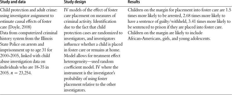
In the US, Doyle (2008) uses administrative data from child protective services and the criminal justice system in Illinois to examine the effects of foster care. He shows first that there is considerable variation between foster care case workers in whether or not a child will be sent to foster care. Moreover, whether a child is assigned to a particular worker is random, depending on who is on duty at the time a call is received. Using this variation, Doyle shows that the marginal child assigned to foster care is significantly more likely to be incarcerated in future. These examples exploit large sample sizes, objective indicators of outcomes, sibling or cohort comparisons, as well as a long follow up period. Some limitations of using existing data include the fact that administrative data sets often contain relatively little background information, and that outcomes are limited to those that are collected in the data bases. Finally, the application process to obtain individual-matched data is often protracted.
Looking forward, the major challenge to research that involves either merging new information to existing data sets, or merging administrative data sets to each other, is that privacy concerns are making it increasingly difficult to obtain data just as it is becoming more feasible to link them. In some cases, access to public use data has deteriorated. For example, for many years, individual level Vital Statistics Natality data from birth certificates included the state of birth, and the county (for counties with over 100,000 population). Since 2005, however, these data elements have been suppressed and it is now necessary to get special permission to obtain US Vital Statistics data with geocodes.
3.2.2 Improvements in the production of administrative data
There are several “first best” potential solutions to these problems. First, creators of large data sets need to be sensitive to the fact that their data may well be useful for addressing questions that they have not envisaged. In order to preserve the ability to use data to answer future questions, it is essential to retain information that can be used for linkage. At a minimum, this should include geographic identifiers at the smallest level of disaggregation that is feasible (for example a Census tract). Ideally, personal identifiers would also be preserved.
Second, more effort needs to be expended in order to make sensitive data available to researchers. A range of mechanisms exist that protect privacy while enabling research:
1 Suppress small cells or merge small cells in public use data files. For example, NCHS data sets such as NHIS could be released with state identifiers for large states, and with identifiers for groups of smaller states.
2 Add small amounts of “noise” to public use data sets, or do data swapping in order to prevent identification of outliers. For example, Cornell University is coordinating the NSF-Census Bureau Synthetic Data Project which seeks to develop public-use “analytically valid synthetic data” from micro datasets customarily accessed at secure Census Research Data Centers.
3 Create model servers. In this approach, users login to estimate models using the true data, but get back output that does not allow individuals to be identified.
4 Data use agreements. The National Longitudinal Survey of Youth and the National Educational Longitudinal Survey have successfully employed data use agreements with qualified users for many years, and without any documented instances of data disclosure.
5 Creation of de-identified merged files. For example, Currie et al. (2009) asked the state of New Jersey to merge birth records with information about the location of pollution sources, and create a de-identified file. This allows them to study the effect of air pollution on infant health.
6 Secure data facilities. The Census Research Data Centers have facilitated access to much confidential data, although researchers who are not located close to the facilities may still face large costs of accessing them.
These approaches to data dissemination have been explored in the statistics literature for more than 20 years (see Dalenius and Reiss (1982)), and have been much discussed at Census (see for example, Reznek (2007)).
3.2.3 Additional issues
We conclude with two new and relatively unexplored data issues. First, how can economists make effective use of the burgeoning literature on biomarkers? These measures have recently been added to existing health surveys, such as the National Longitudinal Study of Adolescent Health data. Biomarkers include not only information about genetic variations but also hormones such as cortisol (which is often interpreted as a measure of stress). It is tempting to think of these markers as potential instrumental variables (Fletcher and Lehrer, 2009). For instance, if it was known that a particular gene was linked to alcoholism, then one might think of using the gene as an instrument for alcoholism. The potential pitfall in this approach is clear if we consider using something like skin color as an instrument in a human capital earnings function-clearly, skin color may predict educational attainment, but it may also have a direct effect on earnings. Just because a variable is “biological” does not mean that it satisfies the criteria for a valid instrument.
A second issue is the evolving nature of what constitutes a “birth cohort.” Improvements in neonatal medicine have meant that stillbirths and fetal deaths that would previously have been excluded from the Census of live births may be increasingly important, e.g. MacDorman et al. (2005). Such a compositional effect on live births may have first-order implications for program evaluation and the long-term effects literature. Indeed, both the right and left tails of the birth weight distribution have elongated over time—in 1970 there were many fewer live births with birthweight either less than 1500 g or over 4000 g. To date there has been little research exploring the implications of these compositional changes.
In summary, there are many secrets currently locked in existing data that researchers do not have access to. Economists have been skillful in navigating the many data challenges inherent in the analysis of long-term (and sometimes latent) effects. Nevertheless, we need to explore ways to make more of these data available, and to more researchers. In many cases, this will be a more cost effective and timely way to answer important questions than carrying out new data collections.
4 Empirical literature: evidence of long term consequences
What is of importance is the year of birth of the generation or group of individuals under consideration. Each generation after the age of 5 years seems to carry along with it the same relative mortality throughout adult life, and even into extreme old age.
Kermack et al. (1934) in The Lancet (emphasis added).
In this section, we summarize recent empirical research findings that experiences before five have persistent effects, shaping human capital in particular. A hallmark of this work is the attention paid to identification strategies that seek to isolate causal effects of the early childhood environment. An intriguing sub-current is the possibility that some of these effects may remain latent during childhood (at least from the researcher’s perspective) until manifested in either adolescence or adulthood. Recently, economists have begun to ask how parents or other investors in human capital (e.g. school districts) respond to early-life shocks, as suggested by the conceptual framework in Section 2.3.
As the excerpt from Kermack et al. (1934) indicates, the idea that early childhood experiences may have important, persistent effects did not originate recently, nor did it first appear in economics. An extensive epidemiological literature has focussed on the early childhood environment, nutrition in particular, and its relationship to health outcomes in adulthood. For a recent survey, see Gluckman and Hanson (2006). This literature has been criticized within epidemiology for credulous empirical comparisons (see, e.g. Rasmussen (2001) or editorial in The Lancet [2001]). Absent clearly-articulated identification strategies, health determinants that are difficult to observe and are therefore omitted from the analysis (e.g., parental concern) are presumably correlated with the treatment and can thereby generate the semblance of ”fetal origins” linkages, even when such effects do not exist.
4.1 Prenatal environment
In the 1990s, David J. Barker popularized and developed the argument that disruptions to the prenatal environment presage chronic health conditions in adulthood, including heart disease and diabetes (Barker, 1992). Growth is most rapid prenatally and in early childhood. When growth is rapid, disruptions to development caused by the adverse environmental conditions may exert life-long health effects. Barker’s “fetal origins” perspective contrasted with the view that pregnant mothers functioned as an effective buffer for the fetus against environmental insults.10
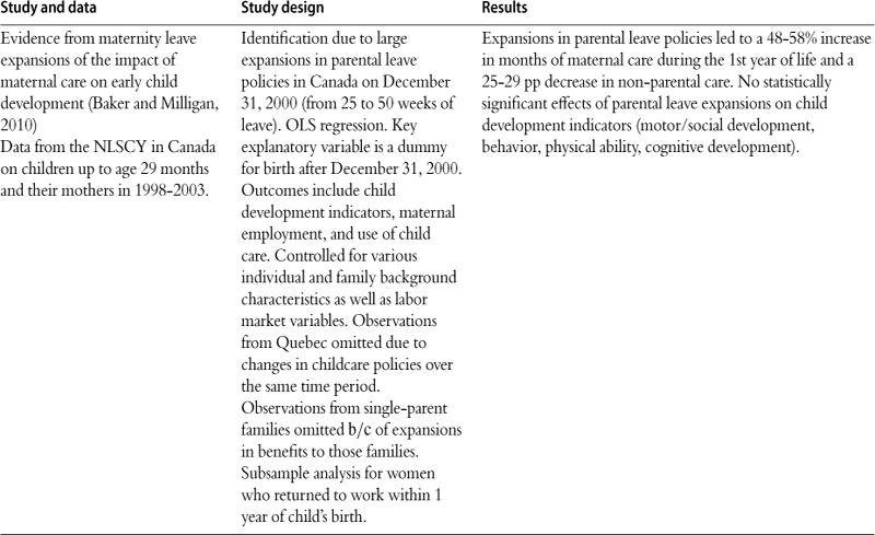
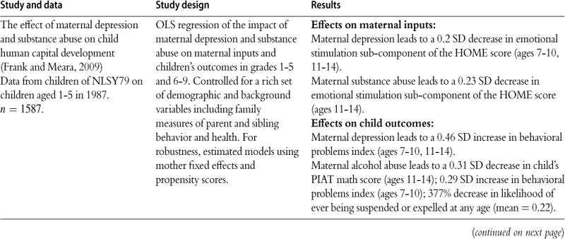
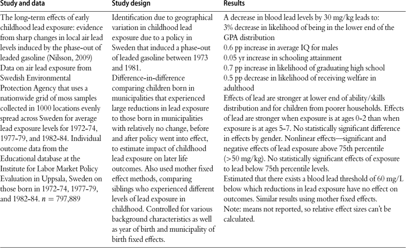
In Table 4, we categorize prenatal environmental exposures into three groups. Specifically, we differentiate among factors affecting maternal and thereby fetal health (e.g. nutrition and infection), economic shocks (e.g. recessions), and pollution (e.g. ambient lead).
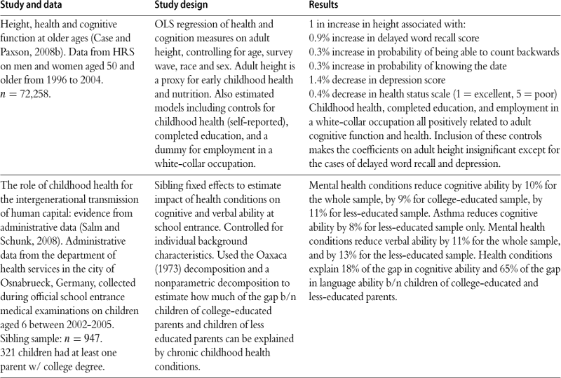
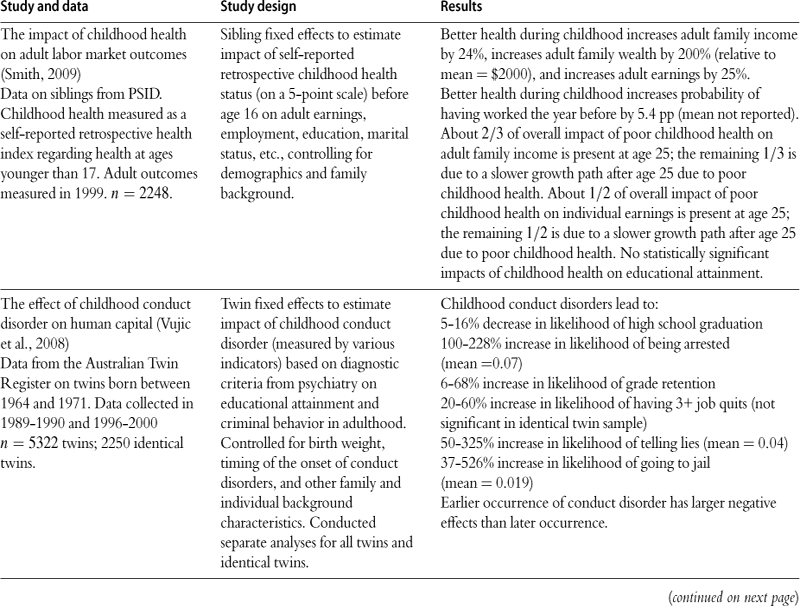
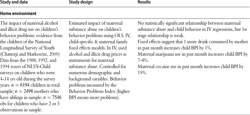
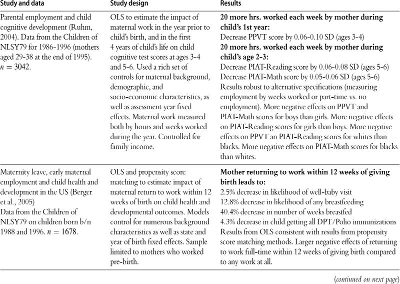
Table 4
Prenatal effects on later child and adult outcomes.
| Study and data | Study design | Results |
| Effects of maternal health | ||
| Is the impact of health shocks cushioned by economic status? The case of low birth weight. Currie and Hyson (1999) NCDS 1958 cohort. N = 11,609 at age 20, 10,267 at age 23, 9402 at age 33. |
Multivariate regression with numerous background and demographic controls (including maternal grandfather’s SES, birth order, and maternal smoking during pregnancy). Key explanatory variables are indicators for LBW, SES, and the interactions. Outcomes measured are the number of O-level passes at age 16 (transcripts collected at age 20), employment, wages and health status at ages 23 and 33. SES assigned using father’s social class in 1958 (or mother’s SES if father is missing). | LBW children are 38–44% less likely to pass Math O-level. LBW females are 25% less likely to pass English O-level tests. LBW females are 16% less likely to be employed full-time at age 23, LBW males are 9% less likely to be employed full-time at age 33. LBW females are 54% more likely to have fair/poor health at age 23, LBW males are 43% more likely to have fair/poor health at age 33. Few significant differences by SES. |
| Returns to birthweight (Behrman and Rosenzweig, 2004). Monozygotic female twins born 1936–1955 from the Minnesota Twins Registry for 1994 and the birth weights of their children. N = 804 twins, and 608 twin-mother pairs. | Twin fixed effects estimates compared to OLS. To explore generalizability of findings from twins sample, weighted the sample using the US singleton distribution of fetal growth rates. | Results from twins sample: 1 oz. per week of pregnancy increase in fetal growth leads to increases of 5%, in schooling attainment; 2% in height; 8% hourly wages. Results from twins sample weighted using singleton distribution: 1 oz. per week of pregnancy increase in fetal growth leads to increase of 5% in schooling attainment; 1.7% in height; no significant effect on wages. OLS underestimates effects of birth weight by 50%. |
| The costs of low birth weight (Almond et al., 2005). Linked birth and infant death files for US for 1983–85,1989-91 and 1995–97. Hospital costs from healthcare cost and utilization project state inpatient database for 1995–2000 in New York and New Jersey. NCHS N = 189,036 twins, 497,139 singletons. HCUP N = 44,410. |
Twin fixed effects to estimate effect of low birth weight (LBW) on hospital costs, health at birth, and infant mortality. Also estimated impact of maternal smoking during pregnancy on health among singleton births, controlling for numerous background and demographic characteristics using OLS and propensity score matching. | Results using twin fixed effects: 1 SD increase in birth weight leads to: 0.08 SD decrease in hospital costs for delivery and initial care 0.03 SD decrease in infant mortality rates 0.03 SD increase in Apgar scores 0.01 SD decrease in use of assisted ventilator after birth (OLS estimates w/out twin fixed effects are 0.51 SD, 0.41 SD, 0.51 SD, 0.25 SD). Results from OLS on effects of maternal smoking: Maternal smoking reduces birth weight by 200 g (6%); increases likelihood that infant is LBW (<2500 g) by more than 100% (mean = 0.061). No statistically significant effects on Apgar score, infant mortality rates, or use of assisted ventilator at birth. |
| The 1918 influenza pandemic and subsequent health outcomes (Almond and Mazumder, 2005). Data from SIPP for 1984–1996. N = 25,169. | Compare cohorts in utero before, during and after Oct. 1918 flu pandemic. Regressions estimate cohort effects including survey year dummies and quadratic in age interacted with survey year. | Individuals born in 1919 are 10% more likely to be in fair or poor health, also increases of 19%, 35%, 13%, 17% in trouble hearing, speaking, lifting and walking. |
| Estimating the impact of large cigarette tax hikes: the case of maternal smoking and infant birth weight (Lien and Evans, 2005). 1990–1997 US Natality files. Data on cigarette taxes from the tax burden on tobacco, various years. | IV using tax hikes in four states as instruments for maternal smoking during pregnancy. Controlled for state and month of conception and background characteristics. | Maternal smoking during pregnancy reduces birth weight by 5.4% and increases likelihood of low birth weight by ~100%. |
| Long term effects of in utero exposure to the 1918 influenza pandemic in the post-1940 US population (Almond, 2006). 1960–1980 US Census data. 1917–1919 Vital Statistics data on mortality. For 1960 n = 114,031, for 1970 n = 308,785, for 1980 n = 471,803. | Estimated effects of in utero influenza exposure by comparing cohorts born immediately before, during, and after the 1918 pandemic and by employing the idiosyncratic geographic variation in intensity of exposure to conduct within-cohort analysis. Exposed cohort = those born in 1919. Surrounding cohorts = those born in 1918 and 1920. Used multivariate regression with dummy for birth cohort = 1919, and a quadratic cohort trend to measure departures in the 1919 birth cohort outcomes from the trend. For geographic comparison, used data on virus strength by week as well as data on epidemic timing by Census division to yield a measure of average pandemic virulence by division. Then estimated multivariate regression including the virulence measure, state and year of birth fixed effects, the infant mortality rate in state and year of birth, and the attrition of birth cohort in the Census data. | Estimation results comparing birth cohorts: The 1919 birth cohort, compared with the cohort trend: was 4%–5% (13%–15% among treated) less likely to complete high school received 0.6%–1.6% fewer years of education had 1%–3% less total income (for males only, 2005 dollars) had 1%–2% lower socioeconomic status index (Duncan index) was 1%–2% more likely to have a disability that limits work (for males only) had 12% higher average welfare payment (for women). Estimates are slightly larger for nonwhite subgroup. Estimation results using geographic variation and state fixed effects: (For the 1919 birth cohort, used average maternal infection rate = 1/3) Maternal infection: reduces schooling by 2.2% reduces probability of high school graduation by 0.05% decreases annual income by 6% reduces socioeconomic status index by 2%–3%. |
| Explaining sibling differences in achievement and behavioral outcomes: the importance of within- and between-family factors (Conley et al., 2007) Data from child development supplement of PSID. N = 1360. | Sibling fixed effects to examine effects of birth weight, birth order, and gender on later outcomes. Cognitive outcomes measured by the Woodcock- Johnson revised tests of achievement. Behavioral outcomes measured by the behavioral problems index (BPI). Control for family- and child-specific characteristics. | No statistically significant effects of birth weight on BPI or on cognitive assessments for whole sample. For blacks, positive effect of birth weight on cognitive assessments. |
| Twin differences in birth weight: the effects of genotype and prenatal environment on neonatal and postnatal mortality (Conley et al., 2006) Data on twin births from the 1995 −97 matched multiple birth database. N = 258,823. |
Twin fixed effects models of effects of birth weight on mortality for same-sex and mixed-sex pairs. | 1 lb increase in birth weight leads to: 9% (10%) reduction in infant mortality for mixed-sex (same-sex) 7% (8%) reduction in neonatal mortality for mixed-sex (same-sex) 2% reduction in post-neonatal mortality for mixed-sex and same-sex. For full-term twins, mixed-sex effects much larger than same-sex effects. |
| Biology as destiny? Short- and long-run determinants of intergenerational transmission of birth weight (Currie and Moretti, 2007). California natality data for children born between 1989 and 2001 and their mothers (ifborn in CA) born between 1970 and 1974. Mothers who are sisters are matched using grandmother’s name. n = 638,497 births. | Examine effect of mother’s birth weight on child’s birth weight in models with grandmother fixed effects. Examine interactions of mother’s birth weight and grandmother’s SES at time of mother’s birth as proxied by income in zip code of mother’s birth. Examine effect of maternal low birth weight on mother’s SES at time she gives birth. | Mother’s low birth weight increases likelihood that child is low birth weight by about 50%. The incidence of child low birth weight is 7% higher if mother was born into high poverty zip code than into low poverty zip code. Children born into poor households are 0.7% more likely to be low birth weight if their mothers were low birth weight; children born into non-poor households are 0.4% more likely to be low birth weight if their mothers were low birth weight (so, poverty raises the probability of transmission of low birth weight by 88%). Being low birth weight is associated with a loss of $110 in future income, on average, on a baseline income of $10,096 (in 1970 dollars). Being low birth weight increases the probability of living in a high-poverty neighborhood by 3% relative to the baseline. Being low birth weight reduces future educational attainment by 0. 1 years. |
| From the cradle to the labor market: the effect of birth weight on adult outcomes (Black et al., 2007). Birth records from Norway for 1967–1997. Dropped congenital defects. Matched to registry data on education and labor market outcomes and to military records. n = 33,366 twin pairs. |
Twin fixed effects, controlling for mother and birth-specific variables. Log(birth weight) is primary independent variable. | 10% increase in birth weight: reduces 1 −year mortality by 13% increases 5 min APGAR score by 0.3% increases probability of high school completion by 1.2% increases full-time earnings by 1%. Male outcomes at age 18–20: 10% increase in birth weight: increases height by 0.3% increases BMI by 0.5% increases IQby 1.1% (scale of 1–9). Effects of mother’s birth weight on child’s birth weight: 10% increase in mother’s birth weight: increases child’s birth weight by 1.5%. |
| The influence of early-life events on human capital, health status and labor market outcomes over the life course (Johnson and Schoeni, 2007) PSID. Adult sample born between 1951 and 1975. N = 5160 people and 1655 families. Child sample 0–12 years old in 1997. N = 1127 mothers and 2239 children. | Sibling fixed effects to estimate impact of maternal smoking during pregnancy on birth outcomes. Also estimated model using OLS, controlling for grandparent smoking in adolescence, maternal birth weight, and paternal smoking, among other background characteristics. | Note: means are not reported, so relative effects cannot be calculated. Effects of income and mother’s birth weight on child’s birth weight: An increase in income of $10,000 raises child’s birth weight by 0.12 lbs if mother was low birth weight (by 0.02 lbs if mother was not low birth weight) for a family with income of $7500 (1997 dollars). Having no health insurance increases the probability of low birth weight by 10 pp. Effects on child health outcomes: (health index 1–100) Low birth weight siblings have a 1. 67 point lower health index. Private health insurance increases health index by 1.02 points. A $10,000 increase in income for families with $15,000-50,000 income increases health index by 0.53 pp. Effects on adult outcomes: Low birth weight siblings: 4. 7 pp more likely to be high school dropouts, have a 3.7 point lower health index (1–100 scale). Low birth weight brothers (sample of males only): are 4.3 pp more likely to have no positive earnings (sig at 10% level) have $2966 less annual earnings (sig at 10% level). |
| Maternal smoking during pregnancy and early child outcomes (Tominey, 2007) Children of NCDS mothers born between 1973 and 2000. n = 2799 mothers and 6291 sibling children. | Sibling fixed effects to estimate impact of maternal smoking during pregnancy on birth outcomes. Also estimated model using OLS, controlling for grandparent smoking in adolescence, maternal birth weight, and paternal smoking, among other background characteristics. | Note: only reporting results from sibling fixed effects regression here. Maternal smoking during pregnancy reduces birth weight by 1.7%. No statistically significant effect of maternal smoking during pregnancy on probability of having a low birth weight child, pre-term gestation, or weeks of gestation. No statistically significant effects of maternal smoking among mothers who quit by month 5 of pregnancy. Larger effects of maternal smoking on birth weight among low educated women. |
| Can a pint per day affect your child’s pay? The effect of prenatal alcohol exposure on adult outcomes (Nilsson, 2008). Data from Swedish LOUISE database on first-born individuals born between 1964 and 1972. n = 353,742. | Swedish natural experiment in which alcohol availability in 2 treatment regions increased sharply as regular grocery stores were allowed to market strong beer for 6 months during 1967 with the minimum age for purchase being 16 (instead of 21). Difference-in-difference-in-difference comparing under-21 mothers with older mothers in treatment and control regions pre-, during, and postexperiment. Baseline estimations focused on children conceived prior to the experiment, but exposed in utero to the experiment. Controlled for quarter and county of birth fixed effects. | DDD results: Years of schooling: decreased by 0.27 (2.1%) years for whole sample; by 0.47 years for males; no statistically significant effect for females. HS graduation: decreased by 0.4% for whole sample; by 10% for males; no stat. significant effect for females. Graduation from higher education: decreased by 16% for whole sample; by 35% for males; no stat. significant effect for females. Earnings at age 32: decreased by 24.1% for whole sample; by 22.8% for males; by 17.7% for females. Probability no income at age 32: increased by 74% whole sample. Proportion on welfare: increased by 90% for whole sample; by 5.1pp for males. |
| Short-, medium- and long-term consequences of poor infant health (Oreopoulos et al., 2008). Data from the Manitoba Center for Health Policy matching provincial health insurance claims with birth records, educational records, and social assistance records. Includes all children born in Manitoba from 1979 to 1985. n = 54,123 siblings and 1742 twins. | Sibling and twin fixed effects. Used three measures of infant health: birth weight, 5-min Apgar score, and gestational length in weeks; used dummies for different categories of the variables to estimate nonlinear effects. Also estimated models using OLS for the whole sample, for the siblings sample, and for the twins sample without family fixed effects. | Note: only reporting results from regressions that included family fixed effects here. BW = birth weight. Relative to Apgar score = 10, BW > 3500 g, gestation 40–41 weeks lower values. Effects on infant mortality: increase infant morality. E.g. in sibling sample (infant mortality = 0.011). Apgar score <6 increases probability of infant mortality by 31.9 pp BW < 1000 g increases probability of infant mortality by 87.2 pp Gestation < 36 weeks increases probability of infant mortality by 11.9 pp. Effect on language arts score (taken in grade 12): Apgar score < 6 decreases test score by 0.1 of SD (sig. at 10% level) BW 2501–3000 g decreases test score by 0.04 of SD Effect on probability of reaching grade 12 by age 17: Apgar score < 6 decreases grade 12 probability by 4.1 pp (sig. at 10%) B W 1001–1500 g decreases grade 12 probability by 14.1 pp Gestation < 36 weeks decreases grade 12 probability by 4.0 pp. Effect on social assistance take-up during ages 18–21.25: BW < 1000 decreases probability of take-up by 21.5 pp. |
| Birth cohort and the black-white achievement gap: the role of health soon after birth (Chay et al., 2009). Data from the national assessment of educational progress long-term trends for 1971–2004. AFQT data from US military for 1976–2001 for male applicants 17–20. n = 2,649,573 white males and n = 1,103,748 black males. Hospital discharge rates from National Health Interview Survey. | Regression of test scores on year, age, and subject fixed effects (separately for blacks and whites) using NAEP-LTT and AFQT test score data. In AFQT test score data, correct for selection bias using inverse probability weighting from Natality and Census data. Estimated regressions separately for blacks and whites and for the North, the South, the Rustbelt, the deep South, and individual states within the South and North. Also estimated difference-in-difference-in-difference (DDD) models, comparing black and white test scores between cohorts born in 1960–62 and 1970–72 in the South relative to the Rustbelt, controlling for region-specific, race-specific age-by-time effects and race-by-region-by-time effects. Used post neonatal mortality rate (PNMR) as a proxy for infant health environment to assess impact of infant health on the test score gap. | NAEP-LTT data: The black-white test score gap declined from 1 SD to 0.6 of SD between 1971 and 2004. The convergence was primarily due to large increases in black test scores in the 1980s. Regression results indicate that the convergence was due to cohort effects, rather than time effects. AFQT data: The black-white gap in AFQT test scores declined by about 19% between the 1962–63 and 1972 birth cohorts. The decline in the gap is about 0.3 SDs greater in the South relative to the Rustbelt between 1960–62 and 1970–72 cohorts. Convergence in PNMR explains 52% of the variation across states in AFQT convergence. Effects of access to hospitals: A 30pp increase in black hospital birth rates from 1962–64 to 1968–70 increases cohort AFQT scores by 7.5 percentile points. A black child who gained admission to a hospital before age 4 had a 0.7-1 SD gain in AFQT score at age 17–18 relative to a black child who did not. |
| Separated at birth: US twin estimates of the effects of birth weight (Royer, 2009) California birth records. n = 3028 same-sex female twin births 1960–1982. Data from early childhood longitudinal study-birth cohort. n = 1496 twin births. | Twin fixed effects, allowing non-linear effects of birth weight. | Twin fixed-effect results: 250 g increase in birth weight leads to: 8.3% decrease in probability of infant mortality 0. 82 day decrease in stay in hospital post-birth 0.02-0.04 of SD increase in mental/motor test score 0. 2% increase in educ. attainment of mother at childbirth 0. 5% increase in child’s birth weight 11% decrease in pregnancy complications. No statistically significant effects of birth weight on adult health outcomes such as hypertension, anemia, and diabetes. No statistically significant effects of birth weight on income-related measures. 200 g increase in birth weight leads to a 0.5 pp increase in probability of being observed in adulthood—small selection bias. Found no statistically significant evidence of compensating or reinforcing parental investments when considering early medical care and breastfeeding. |
| The long-term economic impact of in utero and postnatal exposure to malaria (Barreca, 2010). Malaria mortality from US mortality statistics 1900–1936. n = 1147 state-year observations. Climate data n = 1813 obs. Adult outcomes from 1960 Census. All data merged at state/year of birth level. | IV using fraction of days in “malaria-ideal” temperature range as IV for malaria deaths in state and year. | Note: Only results from the IV regression are reported here. Exposure to 10 additional malaria deaths per 100,000 inhabitants causes 3.4% less years of schooling Exposure to malaria can account for approximately 25% of the difference in years of schooling between cohorts born in high and low malaria states. |
| Long-run longevity effects of a nutrition shock in early life: The Dutch Famine of 1846–47 (Van Den Berg et al., in press). Historical sample of the Netherlands. Exposed cohort born 9/1/1846-6/1/1848. Non-exposed born 9/1/1848-9/1/1855 and 9/1/1837-9/1/1944. | Key independent variable is exposure to famine at birth. Instrument access to food with variations in yearly average real market prices of rye and potatoes for three different regions. Controlled for macroeconomic conditions, infant mortality rates, and individual demographic and socio-economic characteristics. | Results from nonparametric regression: Residual life expectancy at age 50 is 3.1 years shorter for exposed men than for men born after the famine; 1.4 years shorter than for men born before famine. Kolmogorov-Smirnov test suggests that the survival curves after age 50 differ significantly for exposed and control men. Max difference in distribution = 0.15 at age 56. Results from parametric survival models: Exposure to famine at birth for men reduces residual life expectancy at age 50 by 4.2 years. No statistically significant results for women. |
| Maternal stress and child well-being: evidence from siblings (Aizer et al., 2009). National Collaborative Perinatal Project. Births 1959–65 in Providence and Boston. N = 1103 births to 915 women. 163 siblings in sample. | Sibling fixed effects. Estimated effect of deviations from mean cortisol levels (cortisol measures maternal stress) during pregnancy on outcomes. | No significant effects on birth weight or maternal postnatal investments. Exposure to top quartile of cortisol level distribution (relative to the middle) leads to 47% of SD decrease in verbal IQ at age 7 (sign. at 10% level). 1 SD deviation in cortisol levels leads to 26% of SD decrease in educational attainment. Exposure to top quartile of cortisol level distribution (relative to the middle) leads to 51% of SD decrease in educational attainment. |
| The scourge of Asian flu: the physical and cognitive development of a cohort of British children in utero during the Asian Influenza Pandemic of 1957, from birth until age 11 (Kelly, 2009). NCDS 1958 cohort. N = 16,765 at birth, 14,358 at 7,14,069 at 11. | Effect of flu on each cohort member identified using variation in incidence of epidemic by local authority of birth. Epidemic peaked when cohort members were 17–23 weeks gestation. 1 /3 of women of child-bearing age were infected, hence true treatment effect can be estimated by multiplying results by 3. | No statistically significant evidence of reinforcing or compensating parental investments. 1 SD increase in epidemic intensity decreases birth weight by 0.03-0.363 SD; decreases test scores by 0.067 of SD at age 7, by 0.043 of SD at age 11 ; increases detrimental effect of mother preeclampsia from −0.075 to −0.11 SD on birth weight; increases detrimental effect of mother smoking by 0.03 of SD on birth weight; increases detrimental effect of mother under 8 stone weight from −0.54 to −0.61 of SD on birth weight |
| Do lower birth weight babies have lower grades? Twin fixed effect and instrumental variables evidence from Taiwan (Lin and Liu, 2009). Birth Certificate data for Taiwan. High school entrance exam results from Committee of Basic Competence Test. N = 118,658. Twin sample n = 7772. | Twin fixed effects and IV using the public health budget and number of doctors in county where child was born as instruments for child’s birth weight. | Twin FE/IV for mothers w/<9 yrs ed & <25 yrs old Increase in birth weight of 100 g leads to: Increase Chinese score: 0.5%/8.2% Increase English score: 0.3%/8.1%* Increase Math score: 0.7%/12.6% Increase Natural Science score: 0.8%/11.8% Increase Social Science score: 0.4%/4.0%* * means significant at 10% level IV results for other subgroups show smaller/no effects. |
| Poor, hungry and stupid: numeracy and the impact of high food prices in industrializing Britain, 1750–1850 (Baten et al., 2007). Data on age heaping from 1951 to 1881 British Census. Information on poor relieffrom Boyer (1990). | Age heaping is rounding age to nearest 5 or 10. Whipple index (WI) = number of ages that are multiples relative to expected number given uniform age distribution. Regressions use WI as dependent variable. Wheat prices and poor reliefmeasures are independent variables. | During the Revolutionary and Napoleonic Wars, the price of wheat almost doubled—and the number of erroneously reported ages at multiples of 5 doubled from 4% to 8%. Men and women born in decades with higher WI sorted into jobs that had lower intelligence requirements. 1 SD increase in the Whipple index associated with a 2.8% (relative to median earnings) decrease in earnings. |
| Impacts of economic shocks | ||
| Birth weight and income: interactions across generations (Conley and Bennett, 2001) Data from PSID. Two samples: (1) children born 1986–1992, n = 1654; (2) reached 19 by 1992, n = 1388 individuals in 766 families. | Sibling fixed effects. | Low birth weight child who spent 6 years at poverty line is less likely to graduate high school than normal birth weight child who spent 6 years at poverty line. Low birth weight child who spent 6 years with income 5 times the poverty line is as likely to graduate high school as normal birth weight child of same income (significant at 10% level). |
| Economic conditions early in life and individual mortality (Van Den Berg et al., in press). Data from historical sample of the Netherlands on individuals born 1812–1903 with date of death observed by 2000. n = 9276. Merged with historical macro time series data. | Compared individuals born in booms with those born in the subsequent recessions. Controlled for wars and epidemics. | Comparing those born in boom of 1872–1876 with those born in recession of 1877–1881: Boom T|T > 2 = 66.0 years, Recession T|T > 2 = 62.5 years Boom T|T > 5 = 70.8 years, Recession T|T > 5 = 67.5 years Regression results: Boom T|T > 2 is 1.58 years greater than Recession T|T > 2 Notation: T|T > 2 = average lifetime given survival past age 2 T|T > 5 = average lifetime given survival past age 5 |
| Evidence on early-life income and late-life health from America’s Dustbowl era (Cutler et al., 2007). The Health and Retirement Study. N = 8739 people born between 1929 and 1941. Agricultural data from National Agricultural Statistics Service. Income data from Bureau of Economic Analysis. | Measured economic conditions in utero using income and yield from the same calendar year for those born in 3rd or 4th quarter of the year and from the previous calendar year for those born in 1st or 2nd quarter. Regressions include the in utero economic condition measure (log income, log yield), dummy for whether respondent’s father was a farmer and interaction of the dummy with the economic conditions. Controlled for region and year of birth fixed effects, region-specific linear time trends, and region-year infant death and birth rates, and other demographic characteristics. | No statistically significant relationship between poor early-life economic conditions during the Dustbowl and late-life health outcomes such as heart conditions, stroke, diabetes, hypertension, arthritis, psychiatric conditions, etc. |
| Long-run health impacts of income shocks: wine and Phylloxera in 19th century France (Banerjee et al., forthcoming). See paper references for source of data on wine production, number of births, and infant mortality. Department level data on heights from military records 1872–1912. n = 3485 year-departments. | Regional variation in a large negative income shock caused by Phylloxera attacks on French vineyards between 1863 and 1890. Shock dummy equal to 0 pre Phylloxera and after 1890 (when grafting solution found). Dummy equal 1 when wine production < 80% of pre-level. Difference-in-difference comparing children born in affected and unaffected areas before and after. | Decrease in wine production was not compensated by an increase in other agricultural production (e.g. wheat), suggesting that this was truly a large negative income shock. Main outcomes: 3-5% decline in height at age 20 for those born in winegrowing families during the year that their region was affected by Phylloxera. Those born in Phylloxera-affected year are 0.35-0.38 pp more likely to be shorter than 1.56 cm. No statistically significant effects on other measures of health or life expectancy. |
| Impacts of environmental shocks | ||
| Lifespan depends on the month of birth (Doblhammer and Vaupel, 2001) Data on populations of Denmark, Austria, and Australia. Denmark: Longitudinal data based on population registry for 1968–2000 n = 1,371,003. Austria: Data from death certificates for 1988–1996 n = 681,677 Australia: Data from death certificates from 1993–1997 n = 219,820 Also used data on individuals born in Britain who died in Australia: n = 43,074 Data on infant mortality for Denmark |
Used t tests to perform pairwise comparisons between mean age at death by quarter of birth. To test whether the seasonal difference in the risk of death accounts for differences in adult life span by month of birth, calculated monthly deviations from annual death rates and used weighted least squares regression with dummies for month of birth, current month, age since last birthday in months, sex, and birth cohort. To test whether selective survival or debilitation during the 1st year of life explains differences in life expectancy at age 50, calculated monthly death rates during 1st year of life and monthly deviations from annual death rates during 1st year of life; then used a multivariate regression without controls for sex and birth cohort. | Note: Autumn-Spring = average difference in age at death between people born in Autumn (Oct-Dec) and in the Spring (Apr-Jun). Denmark: Mean remaining life expectancy at age 50 = 27.52 years 0. 19 years shorter lifespans for those born in 2nd quarter 0. 12 years longer lifespans for those born in 4th quarter Correlation between infant mortality at time of birth and adult mortality after age 50 = 0.87. Austria: Average age at death = 77.70 years 0. 28 years shorter lifespans for those born in 2nd quarter Austria: average age at death = 77.70 years 0. 28 years shorter lifespans for those born in 2nd quarter 0. 32 years longer lifespans for those born in 4th quarter Additional results shown for specific causes of death. Australia: Mean age of death = 78.00 years for those born in 2nd quarter; mean age of death = 77.65 years for those born in 4th quarter British immigrants born Nov.-Jan. have age of death 0. 36 years higher than natives. Those immigrants born Mar-May have age of death 0.26 years lower than Australian natives. |
| Air quality, infant mortality, and the Clean Air Act of 1970 (Chay and Greenstone, 2003a,b) County-level mortality and natality data 1969–1974. Annual monitor level data on total suspended particles (TSP) from EPA. N = 501 county-years. | Clean Air Act imposed regulations on polluters in counties with TSP concentrations exceeding federal ceilings. Used nonattainment status as an instrument for changes in TSP. Also used regression discontinuity methods to examine effect of TSP on infant mortality. | 1% decline in TSP pollution results in 0.5% decline in infant mortality rate. Most effects driven by reduction of deaths occurring within 1 month of birth. |
| Air pollution and infant health: what can we learn from California’s recent experience? (Currie and Neidell, 2005) Data on pollution from California EPA. Individual-level infant mortality data from California vital statistics 1989–2000. n = 206,353. | Estimated linear models that approximate hazard models, where the risk of death is defined over weeks of life, and length of life is controlled for with a flexible nonparametric spline. Controlled for prenatal and postnatal pollution exposure, weather, child’s age, and numerous other child and family characteristics, as well as month, year, and zip code fixed effects. Examined effects of ozone (O3), carbon monoxide (CO), and particulate matter (PM10) on infant mortality. | 1. 1 unit reduction in postnatal exposure to CO (the actual reduction that occurred in CA in the 1990s) saved 991 infant lives, −4.6% decrease in infant mortality rate. No statistically significant effects of prenatal exposure to any of the pollutants. |
| Prenatal exposure to radioactive fallout (from Chernobyl) and school outcomes in Sweden (Almond et al., 2009). All Swedes born 1983–1988, n = 562,637. Data on radiation from Swedish Geological Survey at parish level. | Three empirical strategies: (1) Cohort comparisons—Compared cohorts in utero before, during, and after Chernobyl with particular focus on cohort 8–25 weeks post conception. (2) Within-cohort comparisons-Use geographic variation in levels of exposure. Define 4 regions, R0 (least exposure), R1, R2, R3. (3) Diff-in-diff sibling comparison—Compared those exposed to radiation in utero 8–25 to siblings who were not. |
Results from (1): Probability of qualifying for high school reduced by 0.2% for cohort in utero during radiation; by 0.6% for cohort in utero 8–25. Grades reduced by 0.4% for cohort in utero during radiation; by 0. 6% for cohort in utero 8–25. Results from (2): (R3 relative to R0) Probability of qualifying for high school reduced by 3.6% for cohort in utero during radiation in R3; by 4% for cohort in utero 8–25 in R3. Grades reduced by 3% for cohort in utero during radiation in R3; by 5.2% for cohort in utero 8–25 in R3. Results from (3): (R3 relative to R0) Difference in probability of qualifying for high school between siblings increased by 6% in R3. Difference in grades between siblings increased by 8% in R3. |
| Air pollution and infant health: lessons from New Jersey (Currie et al., 2009). Pollution data from EPA. Individual-level data on infant births and deaths from the New Jersey Department of Health 1989–2003. n = 283,393 for mother fixed effects models. | Mother fixed effects to estimate impact of exposure to pollution (during and after birth) on infant health outcomes. Air pollution measured from air quality monitors and assigned to each childbased on home address of mother. Also included interactions b/n variable for pollution exposure and maternal smoking as well as other maternal characteristics. Controlled for weather, pollution monitor locations, time trends, seasonal effects, and other background characteristics. | 1 unit change in mean CO exposure during last trimester of pregnancy decreases average birth weight by 0.5%, increases likelihood of low birth weight by 8%, and decreases gestation by 0.2%. 1 unit change in mean CO exposure in first 2 weeks after birth increases likelihood of infant mortality by 2.5%. Estimated that a 1 unit decrease in mean CO exposure in first 2 weeks after birth would save 17.6 per 100,000 lives. Effects of CO exposure on infant health at birth are 2–6 times larger for smokers and mothers who are over age 35. Effects of PM10 (particulate matter) and ozone are not consistently significant across the specifications. |
| Fetal exposures to toxic releases and infant health (Currie et al., 2009) Toxic Release Inventory data at county-year level matched to county-year level natality and infant mortality data. N = 5279. |
Multivariate regression of infant health outcomes on amount of toxic releases in each county and year, controlling for demographic and socio-economic characteristics, mother drinking or smoking during pregnancy, county employment, and county and year fixed effects. Compared effects of developmental toxins to other toxins, and “fugitive” air releases to “stack” air releases (since emissions that go up a smoke stack are more likely to be treated in some way, and hence will affect those in the vicinity less). | An additional thousand pounds per square mile of all toxic releases leads to: 0.02% decrease in length of gestation 0.04% decrease in birth weight 0.1% increase in probability of low birth weight 0.8% increase in probability of very low birth weight 1.3% increase in infant mortality Larger effects for developmental toxins and for fugitive air releases than for other toxins or for stack air releases. A 2-SD increase in lead releases decreases gestation by 0.02% and decreases birth weight by 0.05%. A 2-SD increase in cadmium releases decreases gestation by 0.03%, decreases birth weight by 0. 07%, increases probability of low birth weight by 1. 2%, increases probability of very low birth weight by 1. 4%, and increases infant mortality by 5%. Similar results for toluene, epichlorohydrin. Reductions in releases over 1988–1999 can account for 3.9% of the reduction in infant mortality over the same time period. |
| Traffic congestion and infant health: evidence from E-ZPass (Currie and Walker, 2009) Birth records for Pennsylvania and New Jersey, 1994–2003. Data on housing prices for New Jersey. N = 727,954 for diff-in-diff. N = 232,399 for mother fixed effects. | Identification due to introduction of electronic toll collection (E-ZPass), which reduced traffic congestion and motor vehicle emissions in the vicinity of highway toll plazas. Difference-in-difference, comparing infants born to mothers living near toll plazas to infants born to mothers living near busy roadways (but away from toll plazas), before and after introduction of E-ZPass. Also estimated impacts of exposure to E-ZPass on infant health using mother fixed effects methods. Controlled for various background characteristics, year and month fixed effects, and plaza-specific time trends. Also estimated impact of E-ZPass introduction on housing prices near the toll plaza. |
Results from Difference-in-Difference Method: Reductions in traffic congestion generated by introduction of E-ZPass reduced incidence of premature birth by 10.8% and low birth weight by 11. 8% for children of mothers living w/in 2 km of a toll plaza. For those living w/in 3 km of a toll plaza, effects are 7.3% for premature births and 8.4% for low birth weight. Similar results using mother fixed effects. No effects of E-ZPass introduction on housing prices or demographic composition of mothers living near toll plazas. |
| Caution, Drivers! Children Present. Traffic, Pollution, and Infant Health (Knittel et al., 2009). Traffic data from the freeway performance measurement system. Pollution data from EPA. Birth data from California Dept. of Public Health 2002–2006. N = 373,800. | IV using traffic shocks (due to accidents or road closures) to instrument for air pollution. Preferred specifications include traffic flow, delays, and interactions between traffic and weather. | Note: only results from the IV regression are reported here. 1 unit decrease in exposure to particulate matter (PM10) leads to 5% decrease in infant mortality rate (saves 14 lives per 100,000 births). |
Unless otherwise noted, only results significant at 5% level are reported.
4.1.1 Maternal health
Currie and Hyson (1999) broke ground in economics by exploring whether “fetal origins” (FO) effects were confined to chronic health conditions in adulthood, or might extend to human capital measures. Using the British National Child Development Survey, low birth weight children were more than 25% less likely to pass English and math O-level tests, and were also less likely to be employed. The finding that test scores were substantially affected was surprising, as epidemiologists routinely posited fetal “brain sparing” mechanisms, whereby adverse in utero conditions were parried through a placental triage that prioritized neural development over the body, see, e.g., Scherjon et al. (1996). Furthermore, Stein et al. (1975)’s influential study found no effect of prenatal exposure to the Dutch Hunger Winter on IQ.
Currie and Hyson (1999) were followed by a series of papers that exploited differences in birthweight among siblings and explored their relationship to sibling differences in completed schooling. In relatively small samples (approximately 800 families), Conley and Bennett (2001) found negative but imprecise effects of low birth weight on educational attainment. Statistically significant effects of low birth weight on educational attainment were found when birth weight was interacted with being poor, but in general sample size prevented detection of all but the largest effects (see Section 3.1). Using a comparable sample size, Behrman and Rosenzweig (2004) found the schooling of identical female twins was nearly one-third of a year longer for a pound increase in birth weight (454 grams), with relatively imprecise effects on adult BMI or wages.
In light of the above power concerns, Currie and Moretti (2007) matched mothers to their sisters in half a million birth records from California. Here, low birth weight was found to have statistically significant negative impacts on educational attainment and the likelihood of living in a wealthy neighborhood. However, the estimated magnitudes of the main effects were more modest: low birth weight increased the likelihood of living in a poor neighborhood by 3% and reduced educational attainment approximately one month on average. Like Conley and Bennett (2001), the relationship was substantially stronger for the interaction between low birth weight and being born in poor neighborhoods.
In a sample of Norwegian twins, Black et al. (2007) also found long-term effects of birth weight, but did not detect any heterogeneity in the strength of this relationship by parental socioeconomic status.11 Oreopoulos et al. (2008) find similar results for Canada and Lin and Liu (2009) find positive long term effects of birth weight in Taiwan. Royer (2009) found long-term health and educational effects within California twin pairs, with a weaker effect of birth weight than several other studies, esp. Black et al. (2007). Responsive investments could account for this discrepancy if they differed between California and elsewhere (within twin pairs). Alternatively, there may be more homogeneity with respect to socioeconomic status in Scandinavia than in California. As described in Section 3, Royer (2009) analyzed investment measures directly with the ECLS-B data, concluding that there was no evidence of compensatory or reinforcing investments (see Section 2.2).
Following a literature in demography on seasonal health effects, Doblhammer and Vaupel (2001) and Costa and Lahey (2005) focused on the potential long-term health effects of birth season. A common finding is that in the northern hemisphere, people born in the last quarter of the year have longer life expectancies than those born in the second quarter. Both the availability of nutrients can vary seasonally (particularly historically), as does the likelihood of common infections (e.g., pneumonia). Therefore, either nutrition or infection could drive this observed pattern. Almond (2006) focused on prenatal exposure to the 1918 Influenza Pandemic, estimating that children of infected mothers were 15% less likely to graduate high school and wages were between 5 and 9% lower. Kelly (2009) found negative effects of prenatal exposure to 1957 “Asian flu” in Britain on test scores, though the estimated magnitudes were relatively modest. Interestingly, while birth weight was reduced by flu exposure, this effect appears to be independent of the test score effect. Finally, Field et al. (2009) found that prenatal iodine supplementation raised educational attainment in Tanzania by half a year of schooling, with larger impacts for girls.
4.1.2 Economic shocks
A second set of papers considers economic shocks around the time of birth. Here, health in adulthood tends to be the focus (not human capital), and findings are perhaps less consistent than in the studies of nutrition and infection described above. Van Den Berg et al. (2006)’s basic result is that adult survival in the Netherlands is reduced for those born during economic downturns. In contrast, Cutler et al. (2007) detected no long term morbidity effects in the Health and Retirement Survey data for cohorts born during the Dustbowl era of 1930s. Banerjee et al. (forthcoming) found that shocks to the productive capacity of French vineyards did not have detectable effects on life expectancy or health outcomes, but did reduce height in adulthood. Baten et al. (2007) related variations in grain prices in the decade of birth to numeracy using an ingenious measure based on “age heaping” in the British Censuses between 1851 and 1881. Persons who are more numerate are less likely to round their ages to multiples of 5 or 10. They find that children born in decades with high grain prices were less numerate by this index.
4.1.3 Air pollution
The third strand of the literature examines the effect of pollution on fetal health. Epidemiological studies have demonstrated links between very severe pollution episodes and mortality: one of the most famous focused on a “killer fog” in London, England and found dramatic increases in cardiopulmonary mortality (Logan and Glasg, 1953). Previous epidemiological research on the effects of moderate pollution levels on prenatal health suggests negative effects but have produced inconsistent results. Cross-sectional differences in ambient pollution are usually correlated with other determinants of fetal health, perhaps more systematically than with nutritional or disease exposures considered above. Many of the pollution studies have minimal (if any) controls for these potential confounders. Banzhaf and Walsh (2008) found that high-income families move out of polluted areas, while poor people in-migrate. These two groups are also likely to provide differing levels of (non-pollution) investments in their children, so that fetuses and infants exposed to lower levels of pollution may tend to receive, e.g., better quality prenatal care. If these factors are unaccounted for, this would lead to an upward bias in estimates. Alternatively, certain pollution emissions tend to be concentrated in urban areas, and individuals in urban areas may be more educated and have better access to health care, factors that may improve health. Omitting these factors would lead to a downward bias, suggesting the overall direction of bias from confounding is unclear.
Two studies by Chay and Greenstone (2003a,b) address the problem of omitted confounders by focusing on “natural experiments” provided by the implementation of the Clean Air Act of 1970 and the recession of the early 1980s. Both the Clean Air Act and the recession induced sharper reductions in particulates in some counties than in others, and they use this exogenous variation in levels of pollution at the county-year level to identify its effects. They estimate that a one unit decline in particulates caused by the implementation of the Clean Air Act (recession) led to between five and eight (four and seven) fewer infant deaths per 100,000 live births. They also find some evidence that the decline in Total Suspended Particles (TSPs) led to reductions in the incidence of low birth weight. However, only TSPs were measured at that time, so that they could not study the effects of other pollutants. And the levels of particulates studied by Chay and Greenstone are much higher than those prevalent today; for example, PM10 (particulate matter of 10 microns or less) levels have fallen by nearly 50% from 1980 to 2000.
Several recent studies consider natural experiments at more recently-encountered pollution levels. For example, Currie et al. (2009) use data from birth certificates in New Jersey in which they know the exact location of the mothers residence, and births to the same mother can be linked. They focus on a sample of mothers who live near pollution monitors and show that variations in pollution from carbon monoxide (which comes largely from vehicle exhaust) reduces birth weight and gestation. Currie and Walker (2009) exploit a natural experiment having to do with introduction of electronic toll collection devices (E-ZPass) in New Jersey and Pennsylvania. Since much of the pollution produced by automobiles occurs when idling or accelerating back to highway speed, electronic toll collection greatly reduces auto emissions in the vicinity of a toll plaza. Currie and Walker (2009) compare mothers near toll plazas to those who live near busy roadways but further from toll plazas and find that E-ZPass increased birth weight and gestation. They show that they obtain similar estimates following mothers over time and estimating mother fixed effects models. These papers are notable in part because it has proven more difficult to demonstrate effects of pollution on fetal health than on infant health, as discussed further below. Hence, it appears that being in utero may be protective against at some forms of toxic exposure (such as particulates) but not others.
This literature on the effects of air pollution is closely related to that on smoking. Smoking is, after all, the most important source of indoor air pollution. Medical research has shown that nicotine constricts the oxygen supply to the fetus, so there is an obvious mechanism for smoking to affect infant health. Indeed, there is near unanimity in the medical literature that smoking is the most important preventable cause of low birth weight. Economists have focused on ways to address heterogeneity in other determinants of birth outcomes that are likely associated with smoking. Tominey (2007) found that relative to a conventional multivariate control specification, roughly one-third of the harm from smoking to birth weight is explained by unobservable traits of the mother. Moreover, the reduction in birth weight from smoking was substantially larger for low-SES mothers. In a much larger sample, Currie et al. (2009) showed that smoking significantly reduced birth weight, even when comparisons are restricted to within-sibling differences. Moreover, Currie et al. (2009) document a significant interaction effect between exposure to carbon monoxide exposure and infant health in the production of low birth weight, which may help explain the heterogeneity in birth weight effects reported by Tominey (2007). Aizer and Stroud (2009) note that impacts of smoking on birth weight are generally much smaller in sibling comparisons than in OLS and matching-based estimates. Positing that attenuation bias is accentuated in the sibling comparisons, Aizer and Stroud (2009) use serum cotinine levels as an instrument for measurement error in smoking and find that sibling comparisons yield similar birth weight impacts (around 150 g). Lien and Evans (2005) use increases in state excise taxes as an instrument for smoking and find large effects of smoking on birth weight (182 g) as a result. Using propensity score matching, Almond et al. (2005) document a large decrease in birth weight from prenatal smoking (203 g), but argue that this weight decrease is weakly associated with alternative measures of infant health, such as prematurity, APGAR score, ventilator use, and infant mortality.
Some recently-released data will enable new research on smoking’s short and long-term effects. In 2005, twelve states began using the new US Standard Certificate of Live Birth (2003 revision). Along with other new data elements (e.g., on surfactant replacement therapy), smoking behavior is reported by trimester. It will be useful to consider whether smoking’s impact on birth weight varies by trimester, and also whether smoking is more closely tied to other measures of newborn health if it occurs early versus late in pregnancy. Second, there is relatively little research by economists on the long-term effects of prenatal exposure to smoking. Between 1990 and 2003, there were 113 increases in state excise taxes on cigarettes (Lien and Evans, 2005).12 Since 2005, the American Community Survey records both state and quarter of birth, permitting linkage of these data to the changes in state excise taxes during pregnancy.
Almond et al. (2009) examine the effect of pollution from the Chernobyl disaster on the Swedish cohort that was in utero at the time of the disaster. Since the path of the radiation was very well measured, they can compare affected children to those who were not affected as well as to those born in the affected areas just prior to the disaster. They find that in the affected cohort those who suffered the greatest radiation exposure were 3% less likely to qualify for high school, and had 6% lower math grades (the measure closest to IQ). The estimated effects were much larger within families. A possible interpretation is that cognitive damage from Chernobyl was reinforced by parents.
To summarize, the recent “fetal origins” literature in economics finds substantial effects of prenatal health on subsequent human capital and health. As we discuss in Section 5, this suggests a positive role for policies that improve human capital by affecting the birth endowment. That is, despite being congenital (i.e. present from birth), this research indicates that the birth endowment is malleable in ways that shape human capital. This finding has potentially radical implications for public policy since it suggests that one of the more effective ways to improve children’s long term outcomes might be to target women of child bearing age in addition to focusing on children after birth.
4.2 Early childhood environment
It would be surprising to find that a very severe shock in early childhood (e.g., a head injury, or emotional trauma) had no effect on an individual. Therefore, a more interesting question from the point of view of research is how developmental linkages operating at the individual level affect human capital formation in the aggregate. To answer this question, we need to know how many children are affected by negative early childhood experiences that could plausibly exert persistent effects? How big and long-lasting are the effects of less severe early childhood shocks relative to more severe shocks? Taken together, how much of the differences in adult attainments might be accounted for by things that happen to children between birth and age five? Furthermore, how are these linkages between shocks and outcomes mediated or moderated by third factors? For example, is the effect of childhood lead exposure on subsequent test scores stronger for families of lower socioeconomic status (i.e. is the interaction with SES an important one) and if so why? Alternatively, is the effect of injury mediated by health status, or is the causal pathway a direct one to cognition?
We might also wish to know how parents respond to early childhood shocks. To date, there has been less focus on this question in the early childhood period than in the prenatal period, perhaps because it seems less plausible to hope to uncover a “pure” biological effect of a childhood shock given that children are embedded in families and in society. However, this embeddedness opens the possibility that a richer set of behavioral responses—of the kind considered by economists—might be at play. Furthermore, early childhood admits a wider set of environmental influences than the prenatal period. For example, abuse in early childhood can be distinguished from malnutrition, a distinction more difficult for the in utero period, and these may have quite different effects.
We define early childhood as starting at birth and ending at age five. From an empirical standpoint, early childhood so defined offers advantages and disadvantages over analyses that focus on the prenatal period. Mortality is substantially lower during early childhood than in utero, which reduces the scope for selective attrition caused by environmental shocks to affect the composition of survivors. On the other hand, it is unlikely that environmental sensitivity during early childhood tapers discontinuously at any precise age (including age five). From a refutability perspective, we cannot make sharp temporal comparisons of a cohort “just exposed” to a shock during early childhood to a neighboring cohort “just unexposed” by virtue of its being too old to be sensitive. Moreover, it will often be difficult to know a priori whether prenatal or postnatal exposure is more influential.13 Thus, studies of early childhood exposures tend to emphasize cross-sectional sources of variation, including that at the geographic and individual level. The studies reviewed in this section focus on tracing out the relationships between events in early childhood and future outcomes, and are summarized in Table 5.