
Earnings, Consumption and Life Cycle Choices*
Costas Meghir*, *Yale University, University College London, IFS and IZA
Luigi Pistaferri**, ** Stanford University, NBER, CEPR and IZA
Abstract
We discuss recent developments in the literature that studies how the dynamics of earnings and wages affect consumption choices over the life cycle. We start by analyzing the theoretical impact of income changes on consumption—highlighting the role of persistence, information, size and insurability of changes in economic resources. We next examine the empirical contributions, distinguishing between papers that use only income data and those that use both income and consumption data. The latter do this for two purposes. First, one can make explicit assumptions about the structure of credit and insurance markets and identify the income process or the information set of the individuals. Second, one can assume that the income process or the amount of information that consumers have are known and test the implications of the theory. In general there is an identification issue that has only recently being addressed with better data or better “experiments”. We conclude with a discussion of the literature that endogenizes people’s earnings and therefore change the nature of risk faced by households.
Keywords
Consumption; Risk; Income dynamics; Life cycle
1 Introduction
The objective of this chapter is to discuss recent developments in the literature that studies how the dynamics of earnings and wages affect consumption choices over the life cycle. Labor economists and macroeconomists are the main contributors to this area of research. A theme of interest for both labor economics and macroeconomics is to understand how much risk households face, to what extent risk affects basic household choices such as consumption, labor supply and human capital investments, and what types of risks matter in explaining behavior.1 These are questions that have a long history in economics.
A fruitful distinction is between ex-ante and ex-post household responses to risk. Ex-ante responses answer the question: “What do people do in the anticipation of shocks to their economic resources?”. Ex-post responses answer the question: “What do people do when they are actually hit by shocks to their economic resources?”. A classical example of ex-ante response is precautionary saving induced by uncertainty about future household income (see Kimball, 1990, for a modern theoretical treatment, and Carroll and Samwick, 1998, and Guiso et al., 1992, for empirical tests).2 An example of ex-post response is downward revision of consumption as a result of a negative income shock (see Hall and Mishkin, 1982; Heathcote et al., 2007). More broadly, ex-ante responses to risk may include:3 (a) precautionary labor supply, i.e., cutting the consumption of leisure rather than the consumption of goods (Low, 2005) (b) delaying the adjustment to the optimal stock of durable goods in models with fixed adjustment costs of the (S,s) variety (Bertola et al., 2005); (c) shifting the optimal asset allocation towards safer assets in asset pricing models with incomplete markets (Davis and Willen, 2000); (d) increasing the amount of insurance against formally insurable events (such as a fire in the home) when the risk of facing an independent, uninsurable event (such as a negative productivity shock) increases (known as “background risk” effects, see Gollier and Pratt, 1996, for theory and Guiso et al., 1996, for an empirical test); (e) and various forms of income smoothing activities, such as signing implicit contracts with employers that promise to keep wages constant in the face of variable labor productivity (see Azariadis, 1975 and Baily (1977), for a theoretical discussion and Guiso et al., 2005, for a recent test using matched employer-employee data), or even making occupational or educational choices that are associated with less volatile earnings profiles. Ex-post responses include: (a) running down assets or borrowing at high(er) cost (Sullivan, 2008); (b) selling durables (Browning and Crossley, 2003);4 (c) change (family) labor supply (at the intensive and extensive margin), including changing investment in the human capital of children (Attanasio et al., 2008; Beegle et al., 2004; Ginja, 2010); (d) using family networks, loans from friends, etc. (Hayashi et al., 1996; Angelucci et al., 2010); (e) relocating or migrating (presumably for lack of local job opportunities) or changing job (presumably because of increased firm risk) (Blanchard and Katz, 1992); (f) applying for government-provided insurance (see Gruber, 1997; Gruber and Yelowitz, 1999; Blundell and Pistaferri, 2003; Kniesner and Ziliak, 2002); (g) using charities (Dehejia et al., 2007).
Ex-ante and ex-post responses are clearly governed by the same underlying forces. The ex-post impact of an income shock on consumption is much attenuated if consumers have access to sources of insurance (both self-insurance and outside insurance) allowing them to smooth intertemporally their marginal utility. Similarly, ex-ante responses may be amplified by the expectation of borrowing constraints (which limit the ability to smooth ex-post temporary fluctuations in income). Thus, the structure of credit and insurance markets and the nature of the income process, including the persistence and the volatility of shocks as well as the sources of risk, underlie both the ex-ante and the ex-post responses.
Understanding how much risk and what types of risks people face is important for a number of reasons. First, the list of possible behavioral responses given above suggests that fluctuations in microeconomic uncertainty can generate important fluctuations in aggregate savings, consumption, and growth.5 The importance of risk and of its measurement is well captured in the following quote from Browning et al. (1999):
“in order to...quantify the impact of the precautionary motive for savings on both the aggregate capital stock and the equilibrium interest rate...analysts require a measure of the magnitude of microeconomic uncertainty, and how that uncertainty evolves over the business cycle”.
Another reason to care about risk is for its policy implications. Most of the labor market risks we will study (such as risk of unemployment, of becoming disabled, and generally of low productivity on the job due to health, employer mismatch, etc.) have negative effects on people’s welfare and hence there would in principle be a demand for insurance against them. However, these risks are subject to important adverse selection and moral hazard issues. For example, individuals who were fully insured against the event of unemployment would have little incentive to exert effort on the job. Moreover, even if informational asymmetries could be overcome, enforcement of insurance contracts would be at best limited. For these reasons, we typically do not observe the emergence of a private market for insuring productivity or unemployment risks. As in many cases of market failure, the burden of insuring individuals against these risks is taken on (at least in part) by the government. A classical normative question is: How should government insurance programs be optimally designed? The answer depends partly on the amount and characteristics of risks being insured. To give an example, welfare reform that make admission into social insurance programs more stringent (as heavily discussed in the Disability Insurance literature) reduce disincentives to work or apply when not eligible, but also curtails insurance to the truly eligible (Low and Pistaferri, 2010). To be able to assess the importance of the latter problem is crucial to know how much smoothing is achieved by individuals on their own and how large disability risk is. A broader issue is whether the government should step in to provide insurance against “initial conditions”, such as the risk of being born to bad parents or that of growing up in bad neighborhoods.
Finally, the impact of shocks on behavior also matters for the purposes of understanding the likely effectiveness of stabilization or “stimulus” policies, another classical question in economics. As we shall see, the modern theory of intertemporal consumption draws a sharp distinction between income changes that are anticipated and those that are not (i.e., shocks); it also highlights that consumption should respond more strongly to persistent shocks vis-a-vis shocks that do not last long. Hence, the standard model predicts that consumption may be affected immediately by the announcement of persistent tax reforms to occur at some point in the future. Consumption will not change at the time the reform is actually implemented because there are no news in a plan that is implemented as expected. The model also predicts that consumption is substantially affected by a surprise permanent tax reform that happens today. What allows people to disconnect their consumption from the vagaries of their incomes is the ability to transfer resources across periods by borrowing or putting money aside. Naturally, the possibility of liquidity constraints makes these predictions much less sharp. For example, consumers who are liquidity constrained will not be able to change their consumption at the time of the announcement of a permanent tax change, but only at the time of the actual passing of the reform (this is sometimes termed excess sensitivity of consumption to predicted income changes). Moreover, even an unexpected tax reform that is transitory in nature may induce large consumption responses.
These are all ex-post response considerations. As far as ex-ante responses are concerned, uncertainty about future income realizations or policy uncertainty itself will also impact consumption. The response of consumers to an increase in risk is to reduce consumption—or increase savings. This opens up another path for stabilization policies. For example, if the policy objective is to stimulate consumption, one way of achieving this would be to reduce the amount of risk that people face (such as making firing more costly to firms, etc.) or credibly committing to policy stability. All these issues are further complicated when viewed from a General Equilibrium perspective: a usual example is that stabilization policies are accompanied by increases in future taxation, which consumers may anticipate.
Knowing the stochastic structure of income has relevance besides its role for explaining consumption fluctuations, as important as they may be. Consider the rise in wage and earnings inequality that has taken place in many economies over the last 30 years (especially in the US and in the UK). This poses a number of questions: Does the rise in inequality translate into an increase in the extent of risk that people face? There is much discussion in the press and policy circles about the possibility that idiosyncratic risk has been increasing and that it has been progressively shifted from firms and governments onto workers (one of t-cited example is the move from defined benefit pensions, where firms bear the risk of underperforming stock markets, to defined contribution pensions, where workers do).6 This shift has happened despite the “great moderation” taking place at the aggregate level. Another important issue to consider is whether the rise in inequality is a permanent or a more temporary phenomenon, because a policy intervention aimed at reducing the latter (such as income maintenance policies) differs radically from a policy intervention aimed at reducing the former (training programs, etc.). A permanent rise in income inequality is a change in the wage structure due to, for example, skill-biased technological change that permanently increases the returns to observed (schooling) and unobserved (ability) skills. A transitory rise in inequality is sometimes termed “wage instability”.7
The rest of the chapter is organized as follows. We start off in Section 2 with a discussion of what the theory predicts regarding the impact of changes in economic resources on consumption. As we shall see, the theory distinguishes quite sharply between persistent and transient changes, anticipated and unanticipated changes, insurable and uninsurable changes, and—if consumption is subject to adjustment costs— between small and large changes.
Given the importance of the nature of income changes for predicting consumption behavior, we then move in Section 3 to a review of the literature that has tried to come up with measures of wage or earnings risk using univariate data on wages, earnings or income. The objective of these papers has been that of identifying the most appropriate characterization of the income process in a parsimonious way. We discuss the modeling procedure and the evidence supporting the various models. Most papers make no distinction between unconditional and conditional variance of shocks.8 Others assume that earnings are exogenous. More recent papers have relaxed both assumptions. We also discuss in this section papers that have taken a more statistical path, while retaining the exogeneity assumption, and modeled in various way the dynamics and heterogeneity of risk faced by individuals. We later discuss papers that have explored the possibility of endogenizing risk by including labor supply decisions, human capital (or health) investment decisions, or job-to-job mobility decisions. We confine this discussion to the end of the chapter (Section 5) because this approach is considerably more challenging and in our view represents the most promising development of the literature to date.
In Section 4 we discuss papers that use consumption and income data jointly. Our reading is that they do so with two different (and contrasting) objectives. Some papers assume that the life cycle-permanent income hypothesis provides a correct description of consumer behavior and use the extra information available to either identify the “correct” income process faced by individuals (which is valuable given the difficulty of doing so statistically using just income data) or identify the amount of information people have about their future income changes. The idea is that even if the correct income process could be identified, there would be no guarantee that the estimated “unexplained” variability in earnings represents “true” risk as seen from the individual standpoint (the excess variability represented by measurement error being the most trivial example). Since risk “is in the eye of the beholder”, some researchers have noticed that consumption would reflect whatever amount of information (and, in the first case, whatever income process) people face. We discuss papers that have taken the route of using consumption and income data to extract information about risk faced (or perceived) by individuals, such as Blundell and Preston (1998), Guvenen (2007), Guvenen and Smith (2009), Heathcote et al. (2007), Cunha et al. (2005), and Primiceri and van Rens (2009). Other papers in this literature use consumption and income data jointly in a more traditional way: they assume that the income process is correct and that the individual has no better information than the econometrician and proceed to test the empirical implications of the theory, e.g., how smooth is consumption relative to income. Hall and Mishkin (1982) and Blundell et al. (2008b) are two examples. In general there is an identification issue: one cannot separately identify insurance and information. We discuss two possible solutions proposed in the literature. First, identification of episodes in which shocks are unanticipated and of known duration (e.g., unexpected transitory tax refunds or other payments from the government, or weather shocks). If the assumptions about information and duration hold, all that remains is “insurability”. Second, we discuss the use of subjective expectations to extract information about future income. These need to be combined with consumption and realized income data to identify insurance and durability of shocks.9 The chapter concludes with a discussion of future research directions in Section 6.
2 The impact of income changes on consumption: some theory
In this section we discuss what theory has to say regarding the impact of income changes on consumption.
2.1 The life cycle-permanent income hypothesis
To see how the degree of persistence of income shocks and the nature of income changes affect consumption, consider a simple example in which income is the only source of uncertainty of the model.10 Preferences are quadratic, consumers discount the future at rate ![]() and save on a single risk-free asset with deterministic real return r, β(1 + r) = 1 (this precludes saving due to returns outweighing impatience), the horizon is finite (the consumer dies with certainty at age A and has no bequest motive for saving), and credit markets are perfect. As we shall see, quadratic preferences are in some ways quite restrictive. Nevertheless, this simple characterization is very useful because it provides the correct qualitative intuition for most of the effects of interest; this intuition carries over with minor modifications to the more sophisticated cases. In the quadratic preferences case, the change in household consumption can be written as
and save on a single risk-free asset with deterministic real return r, β(1 + r) = 1 (this precludes saving due to returns outweighing impatience), the horizon is finite (the consumer dies with certainty at age A and has no bequest motive for saving), and credit markets are perfect. As we shall see, quadratic preferences are in some ways quite restrictive. Nevertheless, this simple characterization is very useful because it provides the correct qualitative intuition for most of the effects of interest; this intuition carries over with minor modifications to the more sophisticated cases. In the quadratic preferences case, the change in household consumption can be written as
 (1)
(1)
where a indexes age and t time, ![]() is an “annuity” parameter that increases with age and Ωi,a,t is the consumer’s information set at age a. Despite its simplicity, this expression is rich enough to identify three key issues regarding the response of consumption to changes in the economic resources of the household.
is an “annuity” parameter that increases with age and Ωi,a,t is the consumer’s information set at age a. Despite its simplicity, this expression is rich enough to identify three key issues regarding the response of consumption to changes in the economic resources of the household.
First, consumption responds to news in the income process, but not to expected changes. Only innovations to (current and future) income that arrive at age a (the term E(Yi,a+j,t+j|Ωi,a,t) − E(Yi,a+j,t +j|&i,a−1,t−1)) have the potential to change consumption between age a − 1 and age a. Anticipated changes in income (for which there is no innovation) do not affect consumption. Assistant Professors promoted in February may rent a larger apartment immediately, in the anticipation of the higher salary starting in September. We will record an increase in consumption in February (when the income change is announced), but not in September (when the income change actually occurs). This is predicated on the assumption that consumers can transfer resources from the future to the present by, e.g., borrowing. In the example above, a liquidity constrained Assistant Professor will not change her (rent) consumption at the time of the announcement of a promotion, but only at the time of the actual salary increase. With perfect credit markets, however, the model predicts that anticipated changes do affect consumption when they are announced. In terms of stabilization policies, this means that two types of income changes will affect consumption. First, consumption may be affected immediately by the announcement of tax reforms to occur at some point in the future. Consumption will not change at the time the reform is actually implemented. Second, consumption may be affected by a surprise tax reform that happens today.
The second key issue emerging from Eq. (1) is that the life cycle horizon also plays an important role (the term πα). A transitory innovation smoothed over 40 years has a smaller impact on consumption than the same transitory innovation to be smoothed over 10 years. For example, if one assumes that the income process is i.i.d., the marginal propensity to consume with respect to an income change from (1) is simply πα. Assuming r = 0.02, the marginal propensity to consume out of income shock increases from 0.04 (when A − α = 40) to 0.17 (when A − α = 5), and it is 1 in the last period of life. Intuitively, at the end of the life cycle transitory shocks would look, effectively, like permanent shocks. With liquidity constraints, however, shocks may have similar effects on consumption independently of the age at which they are received.
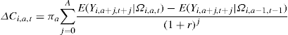
The last key feature of Eq. (1) is the persistence of innovations. More persistent innovations have a larger impact than short-lived innovations. To give a more formalcharacterization of the importance of persistence, suppose that income follows an ARMA(1,1) process:
![]() (2)
(2)
In this case, substituting (2) in (1), the consumption response is given by
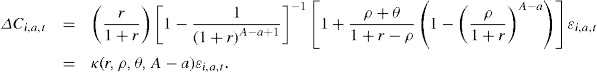
Table 1 below shows the value of the marginal propensity to consume κ for various combinations of ρ, θ, and A − a (setting r = 0.02). A number of facts emerge. If the income shock represents an innovation to a random walk process (ρ = 1, θ = 0), consumption responds one-to-one to it regardless of the horizon (the response is attenuated only if shocks end after some period, say L < A).11 A decrease in the persistence of the shock lowers the value of κ. When ρ = 0.8 (and θ = −0.2), for example, the value of κ is a modest 0.13. A decrease in the persistence of the MA component acts in the same direction (but the magnitude of the response is much attenuated). In this case as well, the presence of liquidity constraints may invalidate the sharp prediction of the model. For example, more and less persistent shocks may have a similar effect on consumption. When the consumer is hit by a short-lived negative shock, she can smooth the consumption response over the entire horizon by borrowing today (and repaying in the future when income reverts to the mean). If borrowing is precluded, short-lived or long-lived shocks have similar impacts on consumption.
The income process (2) considered above is restrictive, because there is a single error component which follows an ARMA(1,1) process. As we discuss in Section 3, a very popular characterization in calibrated macroeconomic models is to assume that income is the sum of a random walk process and a transitory i.i.d. component:
![]() (3)
(3)
![]() (4)
(4)
The appeal of this income process is that it is close to the notion of a Friedman’s permanent income hypothesis income process.12 In this case, the response of consumption to the two types of shocks is:
![]() (5)
(5)
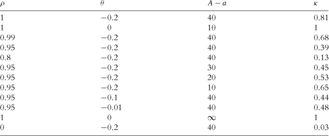
which shows that consumption responds one-to-one to permanent shocks but the response of consumption to a transitory shock depends on the time horizon. For young consumers (with a long time horizon), the response should be small. The response should increase as consumers age. Figure 1 plots the value of the response for a consumer who lives until age 75. Clearly, it is only in the last 10 years of life or so that there is a substantial response of consumption to a transitory shock. The graph also plots for the purpose of comparison the expected response in the infinite horizon case. An interesting implication of this graph is that a transitory unanticipated stabilization policy is likely to affect substantially only the behavior of older consumers (unless liquidity constraints are important—which may well be the case for younger consumers).13
Note finally that if the permanent component were literally permanent (pi,a,t = pi), it would affect the level of consumption but not its change (unless consumers were learning about pi, see Guvenen, 2007).
In the classical version of the LC-PIH the size of income changes does not matter. One reason why the size of income changes may matter is because of adjustment costs: Consumers tend to smooth consumption and follow the theory when expected income changes are large, but are less likely to do so when the changes are small and the costs of adjusting consumption are not trivial. Suppose for example that consumers who want to adjust their consumption upwards in response to an expected income increase need to face the cost of negotiating a loan with a bank. It is likely that the utility loss from not adjusting fully to the new equilibrium is relatively small when the expected income increase is small, which suggests that no adjustment would take place if the transaction cost associated with negotiating a loan is high enough.14 This “magnitude hypothesis” has been formally tested by Scholnick (2010), who use a large data set provided by a Canadian bank that includes information on both credit cards spending as well as mortgage payment records. As in Stephens (2008) he argues that the final mortgage payment represent an expected shock to disposable income (that is, income net of pre-committed debt service payments). His test of the magnitude hypothesis looks at whether the response of consumption to expected income increases depends on the relative amount of mortgage payments. See also Chetty and Szeidl (2007).15
Outside the quadratic preference world, uncertainty about future income realizations will also impact consumption. The response of consumers to an increase in risk is to reduce consumption—or increase savings. This opens up another path for stabilization policies. If the policy objective is to stimulate consumption, one way of achieving this would be to reduce the risk that people face. We consider more realistic preference specifications in the following section.
2.2 Beyond the pih
The beauty of the model with quadratic preferences is that it gives very sharp predictions regarding the impact on consumption of various types of income shocks. For example, there is the sharp prediction that permanent shocks are entirely consumed (an MPC of 1). Unfortunately, quadratic preferences have well known undesirable features, such as increasing risk aversion and lack of a precautionary motive for saving. Do the predictions of this model survive under more realistic assumptions about preferences? The answer is: only qualitatively. The problem with more realistic preferences, such as CRRA, is that they deliver no closed form solution for consumption—that is, there is no analytical expression for the “consumption function” and hence the value of the propensity to consume in response to risk (income shocks) is not easily derivable. This is also the reason why the literature moved on to estimating Euler equations after Hall (1978). The advantage of the Euler equation approach is that one can be silent about the sources of uncertainty faced by the consumer (including, crucially, the stochastic structure of the income process). However, in the Euler equation context only a limited set of parameters (preference parameters such as the elasticity of intertemporal substitution or the intertemporal discount rate) can be estimated.16 Our reading is that there is some dissatisfaction in the literature regarding the evidence coming from Euler equation estimates (see Browning and Lusardi, 1996; Attanasio and Weber, 2010).
Recently there has been an attempt to go back to the concept of a “consumption function”. Two approaches have been followed. First, the Euler equation that describe the expected dynamics of the growth in the marginal utility can be approximated to describe the dynamics of consumption growth. Blundell et al. (2008b), extending Blundell and Preston (1998) (see also Blundell and Stoker, 1994), derive an approximation of the mapping between the expectation error of the Euler equation and the income shock. Carroll (2001) and Kaplan and Violante (2009) discuss numerical simulations in the buffer-stock and Bewley model, respectively. We discuss the results of these two approaches in turn.
2.2.1 Approximation of the Euler equation
Blundell et al. (2008b) consider the consumption problem faced by household i of age a in period t. Assuming that preferences are of the CRRA form, the objective is to choose a path for consumption C so as to:
 (6)
(6)
where Zi,a+j,t+j incorporates taste shifters (such as age, household composition, etc.), and we denote with Ea (.) = E(.|Ωi,a,t). Maximization of (6) is subject to the budget constraint, which in the self-insurance model assumes individuals have access to a risk free bond with real return r
![]() (7)
(7)
![]() (8)
(8)
with Ai,a,t given. Blundell et al. (2008b) set the retirement age after which labor income falls to zero at L, assumed known and certain, and the end of the life cycle at age A. They assume that there is no uncertainty about the date of death. With budget constraint (7), optimal consumption choices can be described by the Euler equation (assuming for simplicity that there is no preference heterogeneity, or υa = 0):
![]() (9)
(9)
As it is, Eq. (9) is not useful for empirical purposes. Blundell et al. (2008b) show that the Euler equation can be approximated as follows:
![]()
where ηi,a,t is a consumption shock with Ea−1(ηi,a,t) = 0, ![]() captures any slope in the consumption path due to interest rates, impatience or precautionary savings and the error in the approximation is
captures any slope in the consumption path due to interest rates, impatience or precautionary savings and the error in the approximation is ![]() .17 Suppose that any idiosyncratic component to this gradient to the consumption path can be adequately picked up by a vector of deterministic characteristics
.17 Suppose that any idiosyncratic component to this gradient to the consumption path can be adequately picked up by a vector of deterministic characteristics ![]() and a stochastic individual element ηi,a
and a stochastic individual element ηi,a
![]()
Assume log income is
![]() (10)
(10)
![]() (11)
(11)
where ![]() represent observable characteristics influencing the growth of income. Income growth can be written as:
represent observable characteristics influencing the growth of income. Income growth can be written as:
![]()
The (ex-post) intertemporal budget constraint is
where A is the age of death and L is the retirement age. Applying the approximation above and taking differences in expectations gives
![]()
where πa is an annuitization factor,  is the share of future labor income in current human and financial wealth, and the error of the approximation is
 ![]() . Then18
. Then18
![]() (12)
(12)
with a similar order of approximation error.19 The random term Ξi,a,t can be interpreted as the innovation to higher moments of the income process.20 As we shall see, Meghir and Pistaferri (2004) find evidence of this using PSID data.
The interpretation of the impact of income shocks on consumption growth in the PIH model with CRRA preferences is straightforward. For individuals a long time from the end of their life with the value of current financial assets small relative to remaining future labor income, ![]() , and permanent shocks pass through more or less completely into consumption whereas transitory shocks are (almost) completely insured against through saving. Precautionary saving can provide effective self-insurance against permanent shocks only if the stock of assets built up is large relative to future labor income, which is to say Ξi,a,t is appreciably smaller than unity, in which case there will also be some smoothing of permanent shocks through self-insurance.
, and permanent shocks pass through more or less completely into consumption whereas transitory shocks are (almost) completely insured against through saving. Precautionary saving can provide effective self-insurance against permanent shocks only if the stock of assets built up is large relative to future labor income, which is to say Ξi,a,t is appreciably smaller than unity, in which case there will also be some smoothing of permanent shocks through self-insurance.
The most important feature of the approximation approach is to show that the effect of an income shock on consumption depends not only on the persistence of the shock and the planning horizon (as in the LC-PIH case with quadratic preferences), but also on preference parameters. Ceteris paribus, the consumption of more prudent households will respond less to income shocks. The reason is that they can use their accumulated stock of precautionary wealth to smooth the impact of the shocks (for which they were saving precautiously against in the first place). Simulation results (below) confirm this basic intuition.
2.2.2 Kaplan and Violante
Kaplan and Violante (2009) investigate the amount of consumption insurance present in a life cycle version of the standard incomplete markets model with heterogenous agents (e.g., Rios-Rull, 1996; Huggett, 1996). Kaplan and Violante’s setup differs from that in Blundell et al. (2008b; BPP) by adding the uncertainty component μα to life expectancy, and by omitting the taste shifters from the utility function. μα is the probability of dying at age a. It is set to 0 for all a < L (the known retirement age) and it is greater than 0 for L ≤ a ≤ A. Their model also differs from BPP by specifying a realistic social security system. Two baseline setups are investigated—a natural borrowing constraint setup (henceforth NBC), in which consumers are only constrained by their budget constraint, and a zero borrowing constraint setup (henceforth ZBC), in which consumers have to maintain non-negative assets at all ages. The income process is similar to BPP.21 Part of Kaplan and Violante’s analysis is designed to check whether the amount of insurance predicted by the Bewley model can be consistently estimated using the identification strategy proposed by BPP and whether BPP’s estimates using PSID and CEX data conform to values obtained from calibrating their theoretical model.
Kaplan and Violante (2009) calibrate their model to match the US data. Survival rates are obtained from the NCHS, the intertemporal discount rate is calibrated to match a wealth-income ratio of 2.5, the permanent shock parameters ![]() and the variance of the initial draw of the process) are calibrated to match PSID data and the variance of the transitory shock
and the variance of the initial draw of the process) are calibrated to match PSID data and the variance of the transitory shock ![]() is set to the 1990–1992 BPP point estimate (0.05). The Kaplan and Violante (2009) model is solved numerically. This allows for the calculation of both the “true”22 and the BPP estimators of the “partial insurance parameters” (the response of consumption to permanent and transitory income shocks).
is set to the 1990–1992 BPP point estimate (0.05). The Kaplan and Violante (2009) model is solved numerically. This allows for the calculation of both the “true”22 and the BPP estimators of the “partial insurance parameters” (the response of consumption to permanent and transitory income shocks).
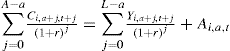
Figure 2 is reproduced from Kaplan and Violante (2009).23 It plots the theoretical marginal propensity to consume for the transitory shocks (upper panels) and the permanent shocks (lower panels) against age (continuous line) and those obtained using BPP’s identification methodology (dashed line). The left panels refer to the NBC environment; the right panels to the ZBC environment. A number of interesting findings emerge. First, in the NBC environment the MPC with respect to transitory shocks is fairly low throughout the life cycle, and similarly to what is shown in Fig. 1, increases over the life cycle due to reduced planning horizon effect. The life cycle average MPC is 0.06. Second, there is considerable insurance also against permanent shock, which increases over the life cycle due to the ability to use the accumulated wealth to smooth these shocks. The life cycle average MPC is 0.77, well below the MPC of 1 predicted by the infinite horizon PIH model.24 Third, the ZBC environment affects only the ability to insure transitory shocks (which depend on having access to loans), but not the ability to insure permanent shocks (which depend on having access to a storage technology, and hence it is not affected by credit restrictions). Fourth, the performance of the BPP estimators is remarkably good. Only in the case of the ZBC environment and a permanent shock does the BPP estimator display an upward bias, and even in that case only very early in the life cycle. According to KV the source of the bias is the failure of the orthogonality condition used by BPP for agents close to the borrowing constraint. It is worth noting that the ZBC environment is somewhat extreme as it assumes no unsecured borrowing. Finally, KV compare the average MPCs obtained in their model (0.06 and 0.77) with the actual estimates obtained by BPP using actual data. As we shall see, BPP find an estimate of the MPC with respect to permanent shocks of 0.64 (s.e. 0.09) and an estimate of the MPC with respect to transitory shocks of 0.05 (s.e. 0.04). Clearly, the “theoretical” MPCs found by KV lie well in the confidence interval of BPP’s estimates. One thing that seems not to be borne out in the data is that theoretically the degree of smoothing of permanent shocks should be strictly increasing and convex with age, while BPP report an increasing amount of insurance with age as a non-significant finding.25 As discussed by Kaplan and Violante (2009), the theoretical pattern of the smoothing coefficients is the result of two forces: a wealth composition effect and a horizon effect. The increase in wealth over the life cycle due to precautionary and retirement motives means that agents are better insured against shocks. As the horizon shortens, the effect of permanent shock resembles increasingly that of a transitory shock.
Figure 2 Age profile of MPC coefficients for transitory and permanent income shocks. Kaplan and Violante (2009)
Given that the response of consumption to shocks of various nature is so different (and so relevant for policy in theory and practice), it is natural to turn to studies that analyze the nature and persistence of the income process.
3 Modeling the income process
In this section we discuss the specification and estimation of the income process. Two main approaches will be discussed. The first looks at earnings as a whole, and interprets risk as the year-to-year volatility that cannot be explained by certain observables (with various degrees of sophistication). The second approach assumes that part of the variability in earnings is endogenous (induced by choices). In the first approach, researchers assume that consumers receive an uncertain but exogenous flow of earnings in each period. This literature has two objectives: (a) identification of the correct process for earnings, (b) identification of the information set—which defines the concept of an “innovation”. In the second approach, the concept of risk needs revisiting, because one first needs to identify the “primitive” risk factors. For example, if endogenous fluctuations in earnings were to come exclusively from people freely choosing their hours, the “primitive” risk factor would be the hourly wage. We will discuss this second approach at the end of the chapter, in Section 5.
There are various models proposed in the literature aimed at addressing the issue of how to model risk in exogenous earnings. They typically model earnings as the sum of a number of random components. These components differ in a number of respects, primarily their persistence, whether there are time- (or age- or experience-) varying loading factors attached to them, and whether they are economically relevant or just measurement error. We discuss these various models in Section 3.1. As said in the Introduction, to have an idea about the correct income process is key to understanding the response of consumption to income shocks.26 As for the issue of information set, the question that is being asked is whether the consumer knows more than the econometrician.27 This is sometimes known as the superior information issue. The individual may have advance information about events such as a promotion, that the econometrician may never hope to predict on the basis of observables (unless, of course, promotions are perfectly predictable on the basis of things like seniority within a firm, education, etc.).28
In general, a researcher’s identification strategy for the correct DGP for income, earnings or wages will be affected by data availability. While the ideal data set is a long, large panel of individuals, this is somewhat a rare event and can be plagued by problems such as attrition (see Baker and Solon, 2003, for an exception). More frequently, researchers have available panel data on individuals, but the sample size is limited, especially if one restricts the attention to a balanced sample (for example, Baker, 1997; MaCurdy, 1982). Alternatively, one could use an unbalanced panel (as in Meghir and Pistaferri, 2004; Heathcote et al., 2007). An important exception is the case where countries have available administrative data sources with reports on earnings or income from tax returns or social security records. The important advantage of such data sets is the accuracy of the information provided and the lack of attrition, other than what is due to migration and death. The important disadvantage is the lack of other information that is pertinent to modeling, such as hours of work and in some cases education or occupation, depending on the source of the data. Even less frequently, one may have available employer-employee matched data sets, with which it may be possible to identify the role of firm heterogeneity separately from that of individual heterogeneity, either in a descriptive way such as in Abowd et al. (1999), or allowing also for shocks, such as in Guiso et al. (2005), or in a more structural fashion as in Postel-Vinay and Robin (2002), Cahuc et al. (2006), Postel-Vinay and Turon (2010) and Lise et al. (2009). Less frequent and more limited in scope is the use of pseudo-panel data, which misses the variability induced by genuine idiosyncratic shocks, but at least allows for some results to be established where long panel data is not available (see Banks et al., 2001; Moffitt, 1993).
3.1 Specifications
The typical specification of income processes found in the literature is implicitly or explicitly motivated by Friedman’s permanent income hypothesis, which has led to an emphasis on the distinction between permanent and transitory shocks to income. Of course things are never as simple as that: permanent shocks may not be as permanent and transitory shocks may be reasonably persistent. Finally, what may pass as a permanent shock may sometimes be heterogeneity in disguise. Indeed these issues fuel a lively debate in this field, which may not be possible to resolve without identifying assumptions. In this section we present a reasonably general specification that encompasses a number of views in the literature and then discuss estimation of this model.
We denote by Yi,a,t a measure of income (such as earnings) for individual i of age a in period t. This is typically taken to be annual earnings and individuals not working over a whole year are usually dropped.29 Issues having to do with selection and endogenous labor supply decisions will be dealt with in a separate section. Many of the specifications for the income process take the form
![]() (13)
(13)
In the above e denotes a particular group (such as education and sex) and Xi,a,t will typically include a polynomial in age as well as other characteristics including region, race and sometimes marital status. From now on we omit the superscript “e” to simplify notation. In (13) the error term ui,a,t is defined such that E(ui,a,t|Xi,a,t) = 0. This allows us to work with residual log income ![]() , where
, where ![]() and the aggregate time effects
and the aggregate time effects ![]() can be estimated using OLS. Henceforth we will ignore this first step and we will work directly with residual log income yi,a,t, where the effect of observable characteristics and common aggregate time trends have been eliminated.
can be estimated using OLS. Henceforth we will ignore this first step and we will work directly with residual log income yi,a,t, where the effect of observable characteristics and common aggregate time trends have been eliminated.
The key element of the specification in (13) is the time series properties of ui,a,t. A specification that encompasses many of the ideas in the literature is
 (14)
(14)
where L is a lag operator such that Lzi,a,t = Zi,a−1,t−1. In (14) the stochastic process consists of an individual specific life cycle trend (a × fi); a transitory shock υi,a,t, which is modeled as an MA process whose lag polynomial of order q is denoted ©q(L); a permanent shock Pp(L)pi,a,t = ζi,a,t, which is an autoregressive process with high levels of persistence possibly including a unit root, also expressed in the lag polynomial of order p, Pp (L); and measurement error mi,a,t which maybe taken as classical i.i.d. or not.
3.1.1 A simple model of earnings dynamics
We start with the relatively simpler representation where the term a × fi is excluded. Moreover we restrict the lag polynomials ©(L) and P(L): it is not generally possible to identify ©(L) and P(L) without any further restrictions. Thus we start with the typical specification used for example in MaCurdy (1982) and Abowd and Card (1989):
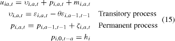 (15)
(15)
with mi,a,t, ζi,a,t and εεi,a,t all being independently and identically distributed and where hi reflects initial heterogeneity, which here persists forever through the random walk (a = 0 is the age of entry in the labor market, which may differ across groups due to different school leaving ages). Generally, as we will show, the existence of classical measurement error causes problems in the identification of the transitory shock process.
There are two principal motivations for the permanent/transitory decompositions: the first motivation draws from economics: the decomposition reflects well the original insights of Friedman (1957) by distinguishing how consumption can react to different types of income shock, while introducing uncertainty into the model.30 The second is statistical: At least for the US and for the UK the variance of income increases over the life cycle (see Fig. 3, which uses consumption data from the CEX and income data from the PSID). This, together with the increasing life cycle variance of consumption points to a unit root in income, as we shall see below. Moreover, income growth (Δyi,a,t) has limited serial correlation and behaves very much like an MA process of order 2 or three: this property is delivered by the fact that all shocks above are assumed i.i.d. In our example growth in income has been restricted to an MA(2).31
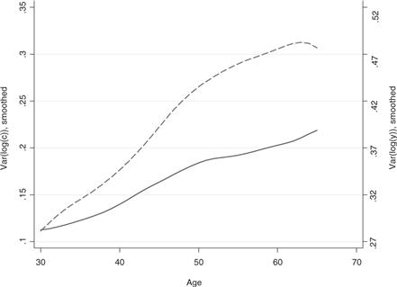
Figure 3 The variance of log income (from the PSID, dashed line) and log consumption (from the CEX, continuous line) over the life cycle.
Even in such a tight specification identification is not straightforward: as we will illustrate we cannot separately identify the parameter θ, the variance of the measurement error and the variance of the transitory shock. But first consider the identification of the variance of the permanent shock. Define unexplained earnings growth as:
![]() (16)
(16)
Then the key moment condition for identifying the variance of the permanent shock is
 (17)
(17)
where q is the order of the moving average process in the original levels equation; in our example q = 1. Hence, if we know the order of serial correlation of log income we can identify the variance of the permanent shock without any need to identify the variance of the measurement error or the parameters of the MA process. Indeed, in the absence of a permanent shock the moment in (17) will be zero, which offers a way of testing for the presence of a permanent component conditional on knowing the order of the MA process. If the order of the MA process is one in the levels, then to implement this we will need at least six individual-level observations to construct this moment. The moment is then averaged over individuals and the relevant asymptotic theory for inference is one that relies on a large number of individuals N.
At this point we need to mention two potential complications with the econometrics. First, when carrying out inference we have to take into account that yi,a,t has been constructed using the pre-estimated parameters dt and β in Eq. (13). Correcting the standard errors for this generated regressor problem is relatively simple to do and can be done either analytically, based on the delta method, or just by using the bootstrap. Second, as said above, to estimate such a model we may have to rely on panel data where individuals have been followed for the necessary minimum number of periods/years (6 in our example); this means that our results may be biased due to endogenous attrition. In practice any adjustment for this is going to be extremely hard to do because we usually do not observe variables that can adequately explain attrition and at the same time do not explain earnings. Administrative data may offer a promising alternative to relying on attrition-prone panel data.
The order of the MA process for υi,a,t will not be known in practice and it has to be estimated. This can be done by estimating the autocovariance structure of gi,a,t and deciding a priori on the suitable criterion for judging whether they should be taken as zero. One approach followed in practice is to use the t-statistic or the F-statistics for higher order autocovariances. However, we need to recognize that given an estimate of q the analysis that follows is conditional on that estimate of q, which in turn can affect inference, particularly for the importance of the variance of the permanent effect ![]() .
.
3.1.2 Estimating and identifying the properties of the transitory shock
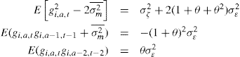
The next issue is the identification of the parameters of the moving average process of the transitory shock and those of measurement error. It turns out that the model is underidentified, which is not surprising: in our example we need to estimate three parameters, namely the variance of the transitory shock ![]() , the MA coefficient θ and the variance of the measurement error
, the MA coefficient θ and the variance of the measurement error ![]() .32 To illustrate the underidentification point suppose that |θ| < 1 and assume that the measurement error is independently and identically distributed. We take as given that q = 1. Then the autocovariances of order higher than three will be zero, whatever the value of our unknown parameters, which is the root of the identification problem. The first and second order autocovariances imply
.32 To illustrate the underidentification point suppose that |θ| < 1 and assume that the measurement error is independently and identically distributed. We take as given that q = 1. Then the autocovariances of order higher than three will be zero, whatever the value of our unknown parameters, which is the root of the identification problem. The first and second order autocovariances imply
 (18)
(18)
The sign of E(gi,a,tgi,a–2,t−2) defines the sign of θ. Taking the two variances as functions of the MA coefficient we note two points. First, ![]() declines and
declines and ![]() increases when θ declines in absolute value. Second, for sufficiently low values of |θ| the estimated variance of the measurement error
increases when θ declines in absolute value. Second, for sufficiently low values of |θ| the estimated variance of the measurement error ![]() may become negative. Given the sign of θ (defined by I in Eq. (18)) this fact defines a bound for the MA coefficient. Suppose for example that θ < 0, we have that
may become negative. Given the sign of θ (defined by I in Eq. (18)) this fact defines a bound for the MA coefficient. Suppose for example that θ < 0, we have that ![]() , where
, where ![]() is the negative value of θ that sets
is the negative value of θ that sets ![]() in (18) to zero. If θ was found to be positive the bounds would be in a positive range. The bounds on θ in turn define bounds on
in (18) to zero. If θ was found to be positive the bounds would be in a positive range. The bounds on θ in turn define bounds on ![]() and
and ![]() .
.
An alternative empirical strategy is to rely on an external estimate of the variance of the measurement error, ![]() . Define the moments, adjusted for measurement error as:
. Define the moments, adjusted for measurement error as:
where ![]() is available externally. The three moments above depend only on θ,
is available externally. The three moments above depend only on θ, ![]() and
and ![]() . We can then estimate these parameters using a Minimum Distance procedure.
. We can then estimate these parameters using a Minimum Distance procedure.
Such external measures can sometimes be obtained through validation studies. For example, Bound and Krueger (1991) conduct a validation study of the CPS data on earnings and conclude that measurement error explains 35 percent of the overall variance of the rate of growth of earnings of males in the CPS. Bound et al. (1994) find a value of 26 percent using the PSID-Validation Study.33
3.1.3 Estimating alternative income processes
Time varying impacts An alternative specification with very different implications is one where
![]() (19)
(19)
where hi is a fixed effect while υi,a,t follows some MA process and mi,a,t is measurement error (see Holtz-Eakin et al., 1988). This process can be estimated by method of moments following a suitable transformation of the model. Define θt = dt/dt−1 and quasi-difference to obtain:
 (20)
(20)
In this model the persistence of the shocks is captured by the autoregressive component of ln Y, which means that the effects of time varying characteristics are persistent to an extent. Given estimates of the levels equation in (20) the autocovariance structure of the residuals can be used to identify the properties of the error term dtΔυi,a,t + mi,a,t−θtmi,a−1,t−1.
Alternatively, the fixed effect with the autoregressive component can be replaced by a random walk in a similar type of model. This could take the form
![]() (21)
(21)
In this model pi,a,t = pi,a−1,t−1 + ζi,a,t as before, but the shocks have a different effect depending on aggregate conditions. Given fixed T a linear regression in levels can provide estimates for dt, which can now be treated as known.
Now define θt = dt/dt−1 and consider the following transformation
![]() (22)
(22)
The autocovariance structure of ln Yi,a,t − θt ln Yi,a−1,t−1 can be used to estimate the variances of the shocks, very much like in the previous examples. We will not be able to identify separately the variance of the transitory shock from that of measurement error, just like before. In general, one can construct a number of variants of the above model but we will move on to another important specification, keeping from now on any macroeconomic effects additive.
It should be noted that (22) is a popular model among labor economists but not among macroeconomists. One reason is that it is hard to use in macro models—one needs to know the entire sequence of prices, address general equilibrium issues, etc.
Stochastic growth in earnings Now consider generalizing in a different way the income process and allow the residual income growth (16) to become
![]() (23)
(23)
where the fi is a fixed effect. The fundamental difference of this specification from the one presented before is that the income growth of a particular individual will be correlated over time. In the particular specification above, all theoretical autocovariances of order three or above will be equal to the variance of the fixed effect fi. Consider starting with the null hypothesis that the model is of the form presented in (15) but with an unknown order for the MA process governing the transitory shock υi,a,t = Θq(L)εi,a,t. In practice we will have a panel data set containing some finite number of time series observations but a large number of individuals, which defines the maximum order of autocovariance that can be estimated. In the PSID these can be about 30 (using annual data). The pattern of empirical autocovariances consistent with (16) is one where they decline abruptly and become all insignificantly different from zero beyond that point. The pattern consistent with (23) is one where the autocovariances are never zero but after a point become all equal to each other, which is an estimate of the variance of fi.
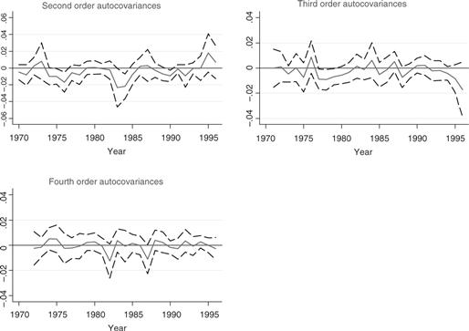
Evidence reported in MaCurdy (1982), Abowd and Card (1989), Topel and Ward (1992), Moffitt and Gottschalk (1994) and Meghir and Pistaferri (2004) and others all find similar results: Autocovariances decline in absolute value, they are statistically insignificant after the 1st or 2nd order, and have no clear tendency to be positive. They interpret this as evidence that there is no random growth term. Figure 4 uses PSID data and plot the second, third and fourth order autocovariances of earnings growth (with 95% confidence intervals) against calendar time. They confirm the findings in the literature: After the second lag no autocovariance is statistically significant for any of the years considered, and there are as many positive estimates as negative ones. In fact, there is no clear pattern in these estimates.
With a long enough panel and a large number of cross sectional observations we should be able to detect the difference between the two alternatives. However, there are a number of practical and theoretical difficulties. First, with the usual panel data, the higher order autocovariances are likely to be estimated based on a relatively low number of individuals. This, together with the fact that the residuals already contain noise from removing the estimated effects of characteristics such as age and even time effects will mean that higher order autocovariances are likely to be imprecisely estimated, even if the variance of fi is indeed non-zero. Perhaps administrative data is one way round this, because we will be observing long run data on a large number of individuals. However, such data is not always available either because it is not organized in a usable way or because of confidentiality issues.
The other issue is that without a clearly articulated hypothesis we may not be able to distinguish among many possible alternatives, because we do not know the order of the MA process, q, or even if we should be using an MA or AR representation, or if the “permanent component” has a unit root or less. If we did, we could formulate a method of moments estimator and, subject to the constraints from the amount of years we observe, we could estimate our model and test our null hypothesis.
The practical identification problem is well illustrated by an argument in Guvenen (2009). Consider the possibility that the component we have been referring to as permanent, pi,a,t, does not follow a random walk, but follows some stationary autoregressive process. In this case the increase in the variance over the life cycle will be captured by the term α × fi. The theoretical autocovariances of gi,a,t will never become exactly zero; they will start negative and gradually increase asymptotically to a positive number which will be the variance of fi, say ![]() . Specifically if pi,a,t = RPi,a−1,t−1 + ζi,a,t with |ρ| < 1, there is no other transitory stochastic component, and the variance of the initial draw of the permanent component is zero, the autocovariances of order k have the form
. Specifically if pi,a,t = RPi,a−1,t−1 + ζi,a,t with |ρ| < 1, there is no other transitory stochastic component, and the variance of the initial draw of the permanent component is zero, the autocovariances of order k have the form
![]() (24)
(24)
As ρ approaches one the autocovariances will approach ![]() . However, the autocovariance in (24) is the sum of a positive and a negative component. Guvenen (2009) has shown, based on simulations, that it is almost impossible in practice with the usual sample sizes to distinguish the implied pattern of the autocovariances from (24) from the one estimated from PSID data. The key problem with this is that the usual panel data that is available either follows individuals for a limited number of time periods, or suffers from severe attrition, which is probably not random, introducing biases. Thus, in practice it is very difficult to identify the nature of the income process without some prior assumptions and without combining information with another process, such as consumption or labor supply.
. However, the autocovariance in (24) is the sum of a positive and a negative component. Guvenen (2009) has shown, based on simulations, that it is almost impossible in practice with the usual sample sizes to distinguish the implied pattern of the autocovariances from (24) from the one estimated from PSID data. The key problem with this is that the usual panel data that is available either follows individuals for a limited number of time periods, or suffers from severe attrition, which is probably not random, introducing biases. Thus, in practice it is very difficult to identify the nature of the income process without some prior assumptions and without combining information with another process, such as consumption or labor supply.
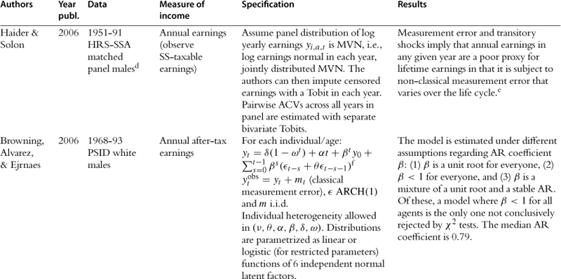
Haider and Solon (2006) provide a further illustration of how difficult it is to distinguish one model from the other. They are interested in the association between current and lifetime income. They write current log earnings as
yi,a,t = hi + afi
and lifetime earnings as (approximately)
log Vi = r − log r + hi + r−1 fi.
The slope of a regression of yi,a,t onto log Vi is:
![]()
Hence, the model predicts that λa should increase linearly with age. In the absence of a random growth term ![]() , λa = 1 at all ages. Figure 5, reproduced from Haider and Solon (2006) shows that there is evidence of a linear growth in λa only early in the life cycle (up until age 35); however, between age 35 and age 50 there is no evidence of a linear growth in λa (if anything, there is evidence that λa declines and one fails to reject the hypothesis λa = 1); finally, after age 50, there is evidence of a decline in λa that does not square well with any random growth term in earnings.
, λa = 1 at all ages. Figure 5, reproduced from Haider and Solon (2006) shows that there is evidence of a linear growth in λa only early in the life cycle (up until age 35); however, between age 35 and age 50 there is no evidence of a linear growth in λa (if anything, there is evidence that λa declines and one fails to reject the hypothesis λa = 1); finally, after age 50, there is evidence of a decline in λa that does not square well with any random growth term in earnings.
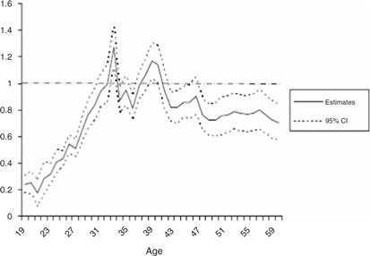
Figure 5 Estimates of λa from Haider and Solon (2006).
Other enrichments/issues The literature has addressed many other interesting issues having to do with wage dynamics, which here we only mention in passing. First, the importance of firm or match effects. Matched employer-employee data could be used to address these issues, and indeed some papers have taken important steps in this direction (see Abowd et al., 1999; Postel-Vinay and Robin, 2002; Guiso et al., 2005).
A number of papers have remarked that wages fall dramatically at job displacement, generating so-called “scarring” effects (Jacobson et al., 1993; von Wachter et al., 2007). The nature of these scarring effects is still not very well understood. On the one hand, people may be paid lower wages after a spell of unemployment due to fast depreciation of their skills (Ljunqvist and Sargent, 1998). Another explanation could be loss of specific human capital that may be hard to immediately replace at a random firm upon re-entry (see Low et al., forthcoming).
3.1.4 The conditional variance of earnings
The typical empirical strategy followed in the precautionary savings literature, in the attempt to understand the role of risk in shaping household asset accumulation choices, typically proceeds in two steps. In the first step, risk is estimated from a univariate ARMA process for earnings (similar to one of those described earlier). Usually the variance of the residual is the assumed measure of risk. There are some variants of this typical strategy—for example, allowing for transitory and permanent income shocks. In the second step, the outcome of interest (assets, savings, or consumption growth) is regressed onto the measure of risk obtained in the first stage, or simulations are used to infer the importance of the precautionary motive for saving. Examples include Banks et al. (2001) and Zeldes (1989). In one of the earlier attempts to quantify the importance of the precautionary motive for saving, Caballero (1990) concluded −using estimates of risk from MaCurdy (1982)—that precautionary savings could explain about 60% of asset accumulation in the US.
A few recent papers have taken up the issue of risk measurement (i.e., modeling the conditional variance of earnings) in a more complex way. Here we comment primarily on Meghir and Pistaferri (2004).34
Meghir and Pistaferri (2004) Returning to the model presented in Section 3.1.1 we can extend this by allowing the variances of the shocks to follow a dynamic structure with heterogeneity. A relatively simple possibility is to use ARCH(1) structures of the form
![]() (25)
(25)
where Et–1 (.) denotes an expectation conditional on information available at time t − 1. The parameters are all education-specific. Meghir and Pistaferri (2004) test whether they vary across education. The terms γt and ϕt are year effects which capture the way that the variance of the transitory and permanent shocks change over time, respectively. In the empirical analysis they also allow for life cycle effects. In this specification we can interpret the lagged shocks (εi,a−1,t−1, ζi,a−1,t−1) as reflecting the way current information is used to form revisions in expected risk. Hence it is a natural specification when thinking of consumption models which emphasize the role of the conditional variance in determining savings and consumption decisions.
The terms v¿ and ξ; are fixed effects that capture all those elements that are invariant over time and reflect long term occupational choices, etc. The latter reflects permanent variability of income due to factors unobserved by the econometrician. Such variability may in part have to do with the particular occupation or job that the individual has chosen. This variability will be known by the individuals when they make their occupational choices and hence it also reflects preferences. Whether this variability reflects permanent risk or not is of course another issue which is difficult to answer without explicitly modeling behavior.35
As far as estimating the mean and variance process of earnings is concerned, this model does not require the explicit specification of the distribution of the shocks; moreover the possibility that higher order moments are heterogeneous and/or follow some kind of dynamic process is not excluded. In this sense it is very well suited for investigating some key properties of the income process. Indeed this is important, because as discussed earlier the properties of the variance of income have implications for consumption and savings.
However, this comes at a price: first, Meghir and Pistaferri (2004) need to impose linear separability of heterogeneity and dynamics in both the mean and the variance. This allows them to deal with the initial conditions problem without any instruments. Second, they do not have a complete model that would allow them to simulate consumption profiles. Hence the model must be completed by specifying the entire distribution.
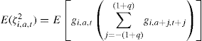
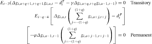
Identification of the ARCH process If the shocks ε and ζ were observable it would be straightforward to estimate the parameters of the ARCH process in (25). However they are not. What we do observe (or can estimate) is gi,a,t = Δmi,a,t + (1+θL) Δεi,a,t + ζi,a,t. To add to the complication we have already argued that θ is not point identified. Nevertheless the following two key moment conditions identify the parameters of the ARCH process, conditional on the unobserved heterogeneity (η and ξ):
 (26)
(26)
The important point here is that it is sufficient to know the order of the MA process q.36 We do not need to know the parameters themselves. The parameter θ that appears in (26) for the transitory shock is just absorbed by the time effects on the variance or the heterogeneity parameter. Hence measurement error, which prevents the identification of the MA process does not prevent identification of the properties of the variance, so long as such error is classical.
The moments above are conditional on unobserved heterogeneity; to complete identification we need to control for that. As the moment conditions demonstrate, estimating the parameters of the variances is akin to estimating a dynamic panel data model with additive fixed effects. Typically we should be guided in estimation by asymptotic arguments that rely on the number of individuals tending to infinity and the number of time periods being fixed and relatively short.
One consistent approach to estimation would be to use first differences to eliminate the heterogeneity and then use instruments dated t − 3 for the transitory shock and dated t − q − 4 for the permanent one. In this case the moment conditions become
 (27)
(27)
where Δxt = xt − xt−1. In practice, however, as Meghir and Pistaferri (2004) found out, lagged instruments suggested above may be only very weakly correlated with the entities in the expectations above. This means that the rank condition for identification is not satisfied and consequently the ARCH parameters may not be identifiable through this approach. An alternative may be to use a likelihood approach, which will exploit all the moments implied by the specification and the distributional assumption; this however may be particularly complicated. A convenient approximation may be to use a within group estimator on (26). This involves subtracting the individual mean of each expression on the right hand side, i.e. just replace all expressions in (26) by quantities where the individual mean has been removed. For example gi,a+q+1,t+q+1gi,a,t is replaced by ![]() . Nickell (1981) and Nerlove (1971) have shown that this estimator is inconsistent for fixed T. Effectively this implies that the estimates may be biased when T is short because the individual specific mean may not satisfy the moment conditions for short T. In practice this estimator will work well with long panel data. Meghir and Pistaferri use individuals observed for at least 16 periods. Effectively, while ARCH effects are likely to be very important for understanding behavior, there is no doubt that they are difficult to identify. A likelihood based approach, although very complex, may ultimately prove the best way forward.
. Nickell (1981) and Nerlove (1971) have shown that this estimator is inconsistent for fixed T. Effectively this implies that the estimates may be biased when T is short because the individual specific mean may not satisfy the moment conditions for short T. In practice this estimator will work well with long panel data. Meghir and Pistaferri use individuals observed for at least 16 periods. Effectively, while ARCH effects are likely to be very important for understanding behavior, there is no doubt that they are difficult to identify. A likelihood based approach, although very complex, may ultimately prove the best way forward.
Other approaches
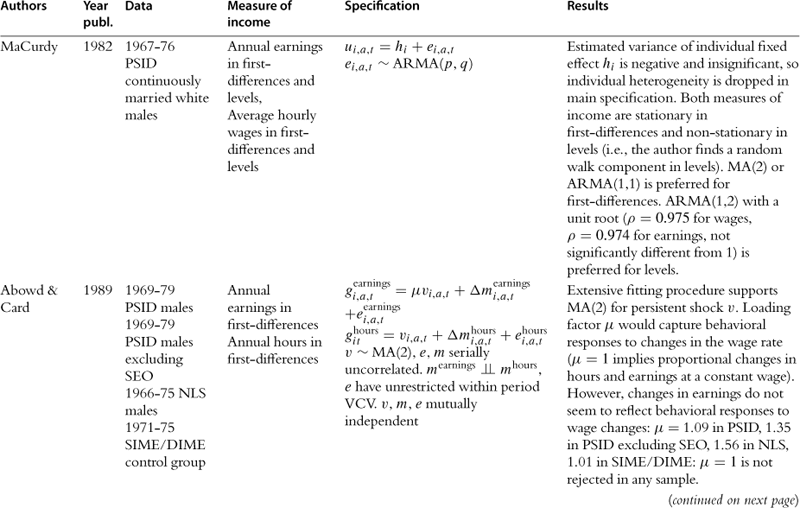
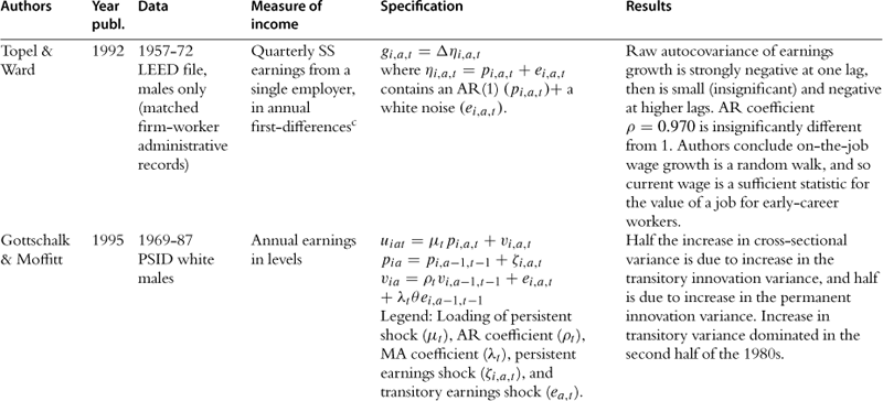
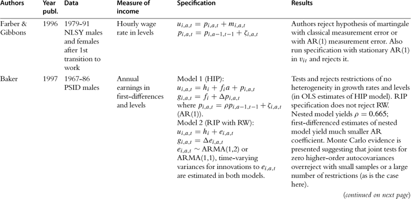
3.1.5 A summary of existing studies
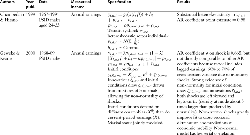
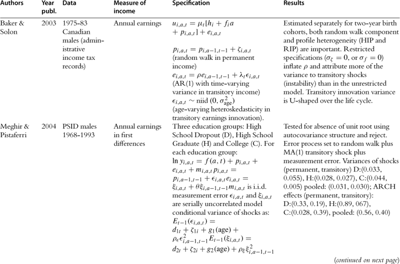
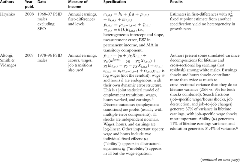
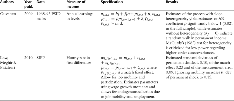
In this section we provide a summary of the key studies in the literature.37 Most of the information is summarized in Table 2, but we also offer a brief description of the key results of the papers in the text. Some of the earliest studies are those of Hause (1980), who was investigating the importance of on-the-job training, and Lillard and Willis (1978), who were interested in earnings mobility. Both find an important role for unobserved heterogeneity and conclude that the process of income is stationary. Hause used the idea of heterogeneous income profiles, which later played a central role in the debate in this literature.
Table 2

aAuthors cut sample by race (black/white).
bNo covariates, so profile heterogeneity captures differences across education groups (focus is on low education workers).
cI.e., gi,a,t = yi,a,t − yi,a−4,t−4 where t indexes quarters.
e> Sample average estimated ACVs pooled over full earnings history (from bivariate Tobit procedures) are very close to results from uncensored data in other studies (Baker and Solon, 2003, Bohlmark and Lindquist, 2006): ACV1 = 0.89, ACV2 = 0.82, ACV3 = 0.78, ACV4 = 0.75, ACV5 = 0.72, ACV6 = 0.69.
f[δ] = “long-run” average earnings; [ω] = inverse speed of convergence to “long-run” average earnings; [a] = linear time trend; [β] = AR(1) coefficient; [θ] = MA(1) coefficient; [ε] = ARCH WN, with constant η, ARCH coefficient ![]() .
.
gParametrization of the model makes it difficult to compare point estimates to other results from the literature. Results for impulse-response to particular shocks are interesting results, but the less detailed models in the income-process literature reviewed here typically present unconditional dynamic behavior rather than distinguishing particular shocks.
h“Joint” in the sense that it is more complex than the univariate earnings processes presented here, but still based only on labor market behavior; “statistical” in the sense that the model’s structural equations are not derived from utility maximization.
Following these papers are two of the most important works in this literature, namely MaCurdy (1982) and Abowd and Card (1989). Both use PSID data for ten years, but covering different time periods. Abowd and Card also use NLS data and data from an income maintenance experiment. The emphasis on these papers is precisely to understand the time series properties of earnings and extract information relating to the variance of the shocks. They both conclude that the best representation of earnings is one with a unit root in levels and MA(2) in first differences. Abowd and Card go further and also model the time series properties of hours of work jointly with earnings, potentially extracting the extent to which earnings fluctuations are due to hours fluctuations. The papers by Low et al. (forthcoming) and Altonji et al. (2009), which explicitly make the distinction between shocks and endogenous responses to shocks, can be seen as related to this work. Similar conclusions are reached by Topel and Ward (1992) using matched firm-worker administrative records spanning 16 years. They conclude that earnings are best described by a random walk plus an i.i.d. error.
In an important paper Gottschalk and Moffitt (1995) use the permanent-transitory decomposition to fit data on earnings and to try to understand the relative importance of the change in the permanent and transitory variance in explaining the changes in US inequality over the 1980s and 1990s. Their permanent component is defined to be a random walk with a time varying variance. The transitory component is an AR(1), also with time varying variance. Both variances were shown to increase over time. They also consider a variety of other models including most importantly the random growth model, where age is interacted with a fixed effect. As we have already explained, this is an important alternative to the random walk model because they both explain the increase in variance of earnings with age, but have fundamentally different economic implications. In their results the two models fit equally well the data38. Based on earlier results by Abowd and Card (1989), Gottschalk and Moffitt choose the random walk model as their vehicle for analysis of inequality and mobility patterns in the data.
Farber and Gibbons (1996) provide a structural interpretation of wage dynamics. The key idea here is that firms publicly learn the worker’s ability and at each point in time the wage is set equal to the conditional expectation of workers’ productivity. Among other results this implies that wage levels follow a martingale. The result is however fragile; for example, if heterogeneous returns to experience are allowed for, the martingale result no longer holds. Their results indeed reject the martingale hypothesis. The model is quite restrictive, because it does not allow for the incumbent firm to have superior information as in Acemoglu and Pischke (1998). Moreover, given the specification in levels (rather than in logs), the relevance of this paper to the literature we are discussing here is mainly because of its important attempt to offer a structural interpretation to wage dynamics rather than for its actual results.
Baker (1997) compares results of fitting the profile heterogeneity model39 to the one where a unit root is allowed for. He fits the levels model to the level of autocovariances of log earnings. When no profile heterogeneity is allowed for, the model displays a unit root. However, when profile heterogeneity is allowed for, the unit root becomes an autoregressive coefficient of about 0.6. Thus, clearly, the unit root is required, when heterogeneity is not allowed for to explain the long term persistence and presumably the increasing variance over the life cycle. However, this can be captured equally well by the profile heterogeneity. As remarked by Gottschalk and Moffitt, and Baker himself, the profile heterogeneity model, as specified by Baker, will imply autocovariances that are increasing with the square of experience/age.40 However, Baker does not seem to exploit this pattern because he fits the autocovariance structure without conditioning on age or potential experience. This may reduce the ability to reject the profile heterogeneity model in favor of the unit root one. Nevertheless, with his approach he finds that both the unit root model and the profile heterogeneity model fit the data similarly. However, when estimating the encompassing model, ui,a,t = hi + a χ fi + pi,a,t with Pi,a,t = ρPi,a−1,t−1 + ζi,a,t, ρ, the coefficient on the AR component is significantly lower than 1, rejecting the unit root hypothesis; moreover the variance of fi is significantly different from zero. On the basis of this, the best fitting model would be heterogeneous income profiles with a reasonably persistent transitory shock. Nevertheless, there still is a puzzle: the autocovariances of residual income growth of order higher than two are all very small and individually insignificant. Baker directly tests that these are indeed jointly zero and despite the apparent insignificance of all of them individually he rejects this hypothesis and concludes that the evidence against the unit root and in favor of the profile heterogeneity model is strong. We suspect that his may be due to the way inference was carried out: Meghir and Pistaferri (2004) also test that all autocovariances of order 3 or more are zero (in the PSID) and they fail to reject this with a p-value of 12%.41 Perhaps the reason for this difference with Baker is that Meghir and Pistaferri use the block bootstrap, thus bypassing the problem of estimating the covariance matrix of the second order moments using the fourth order ones and allowing for more general serial correlation.
The unit root model is particularly attractive for understanding such phenomena as the increase in the variance of consumption over the life cycle, as originally documented by Deaton and Paxson (1994); the fact that mobility in income exceeds mobility in consumption (Jappelli and Pistaferri, 2006); and the fact that the consumption distribution is more lognormal than the income distribution (Battistin et al., 2009). However, the heterogeneous income profiles model is also attractive from the point of view of labor economics. It is well documented that returns to education and experience tend to increase with ability indicators. Such ability indicators are either unobserved in data sets used for studying earnings dynamics or are simply inadequate and not used. There is no real reason why the two hypotheses should be competing and they are definitely not logically inconsistent with each other. Indeed a model with a unit root process and a transitory component as well as a heterogeneous income profile is identifiable.
Specifically, Baker and Solon (2003) estimate a model along the lines of the specification in (21), which allows both for profile heterogeneity and imposes a random walk on the permanent component, as well as an AR(1) transitory one. Their rich model is estimated with a large Canadian administrative data set. There is enough in their model to allow for the possibility that individual components are unimportant. For example the variance of the permanent shock could be estimated to be zero, in which case the model would be one of profile heterogeneity with an autoregressive component, very much like in Baker (1997). Yet the variance of the permanent shock is very precisely estimated and indeed quite large (0.007). Thus these authors find clear evidence (on Canadian data) of both a permanent shock and of long run heterogeneity in the growth profiles. Thinking of the permanent shocks as uncertainty and profile heterogeneity as information known by the individual at the start of life, their estimation provides an interesting balance between the amount of wage variance due to uncertainty and that due to heterogeneity: on the one hand their estimate is a quarter that of Meghir and Pistaferri (2004); on the other hand it is still substantial from a welfare perspective and in terms of its implications for precautionary savings.
Meghir and Pistaferri (2004) adopt the unit root model with MA transitory shocks and measurement error, after testing the specification and finding it acceptable. With their approach they do not find evidence of profile heterogeneity. They also allow for the variances of the shocks to depend on age, time and unobserved heterogeneity as well as ARCH effects. The latter are important because they reflect the volatility of uncertainty. In their model they thus allow heteroskedasticity due to permanent heterogeneity to compete with the impact of volatility shocks. They find very large ARCH effects both for the permanent and the transitory shock, implying large effects on precautionary savings, over and above the effects due to the average variance of the shocks. They also find strong evidence of permanent heterogeneity in variances. One interpretation is that there is considerable uncertainty in income profiles, as expressed by the random walk, but there is also widespread heterogeneity in the distributions from which the permanent and transitory income shocks are drawn. Indeed this idea of heterogeneity was taken up by Browning et al. (2006) who estimate an income process with almost all aspects being individual-specific. They conclude that the nature of the income process varies across individuals, with some being best characterized by a unit root in the process, while others by a stationary one.
Clearly the presence of a random walk in earnings is controversial and has led to a voluminous amount of work. This is not because of some nerdy or pedantic fixation with the exact time series specification of income but is due to the importance of this issue for asset accumulation and welfare.42
Guvenen (2009) compares what he calls a HIP (heterogeneous income profiles) income process and a RIP (restricted income profiles) income process and their empirical implications. The (log) income process (in a simplified form) is as follows:
![]()
with an initial condition equal to 0.
The estimation strategy is based on minimizing the “distance” between the elements of the (T χ T) empirical covariance matrix of income residuals in levels and its counterpart implied by the model described above (where income residuals ![]() are obtained regressing yi,a,t on
are obtained regressing yi,a,t on ![]() ).43 The main findings are as follows. First, mis-specification of a HIP process as a RIP process results in a biased estimation of the persistence parameter ρ and an overestimation of
).43 The main findings are as follows. First, mis-specification of a HIP process as a RIP process results in a biased estimation of the persistence parameter ρ and an overestimation of ![]() . The estimates of ρ are much smaller for HIP (ρ = 0.82) compared to RIP (ρ = 0.99−insignificantly different from 1). When estimating HIP models, the dispersion of income profiles
. The estimates of ρ are much smaller for HIP (ρ = 0.82) compared to RIP (ρ = 0.99−insignificantly different from 1). When estimating HIP models, the dispersion of income profiles ![]() is significant. This dispersion is higher for more educated groups. Finally, 65 to 80 percent of income inequality at the age of retirement is due to heterogeneous profiles.
is significant. This dispersion is higher for more educated groups. Finally, 65 to 80 percent of income inequality at the age of retirement is due to heterogeneous profiles.
Hryshko (2009), in an important paper, sets out to resolve the random walk vs. stochastic growth process controversy by carrying out Monte Carlo simulations and empirical analysis on PSID data. First, he generates data based on a process with a random walk and persistent transitory shocks. He then fits a (misspecified) model assuming heterogenous age profiles and an AR(1) component and finds that the estimated persistence of the AR component is biased downwards and that there is evidence for heterogeneous age profile. In the empirical data he finds that the model with the random walk cannot be rejected, while he finds little evidence in support of the model with heterogeneous growth rates. While these results are probably not going to be viewed as conclusive, what is clear is that the encompassing model of, say, Baker (1997) may not be a reliable way of testing the competing hypotheses. It also shows that the evidence for the random walk is indeed very strong and reinforces the results by Baker and Solon (2003), which support the presence of a unit root as well as heterogeneous income profiles.
Most approaches described above have been based on quite parsimonious time series representations. However three papers stand out for their attempt to model the process in a richer fashion: Geweke and Keane (2000) and Chamberlain and Hirano (1999) use a Bayesian approach and allow for more complex dynamics and (in the latter) for heterogeneity in the dynamics of income; Browning et al. (2006) emphasize the importance of heterogeneity even more. Specifically, Geweke and Keane (2000) follow a Bayesian approach to model life cycle earnings based on the PSID, with the primary motivation of understanding income mobility and to improve the fit vis-à-vis earlier mobility studies, such as the one by Lillard and Willis (1978). Their modeling approach is very flexible, allowing for lagged income, serially correlated shocks and permanent unobserved characteristics. They find that at any point in time about 60–70% of the variance in earnings is accounted for by transitory shocks that average out over the life cycle. But the result they emphasize most is the fact that the shocks are not normal and that allowing for departure from normal heteroskedastic shocks is crucial for fitting the data. In this respect their results are similar to those of Meghir and Pistaferri (2004), who allow for ARCH effects. Nevertheless, the interpretation of the two models is different, because of the dynamics in the variance allowed by the latter.
Similar to Geweke and Keane, Chamberlain and Hirano (1999) also use a Bayesian approach to estimate predictive distributions of earnings, given past histories; they also use data from the PSID. They motivate their paper explicitly by thinking of an individual who has to predict future income when making consumption plans. The main difference of their approach from that of Geweke and Keane is that they allow for heteroskedastic innovations to income and heterogeneity in the dynamics of earnings. They find that the shock process has a unit root when the serial correlation coefficient is constrained to be one for all individuals. When it is allowed to be heterogeneous it is centered around 0.97 with a population standard deviation of 0.07, which implies about half individuals having a unit root in their process.
Browning et al. (2006) extend this idea further by allowing the entire income process to be heterogeneous. Their model allows for all parameters of the income process to be different across individuals, including a heterogeneous income profile and a heterogeneous serial correlation coefficient restricted to be in the open interval (0, 1). This stable model is then mixed with a unit root model, with some mixing probability estimated from the data. This then implies that with some probability an individual faces an income process with a unit root; alternatively the process is stationary with heterogenous coefficients. They estimate their model using the same PSID data as Meghir and Pistaferri (2004) and find that the median AR(1) coefficient is 0.8, with a proportion of individuals (about 30%) having an AR(1) coefficient over 0.9. They attribute their result to the fact that they have decoupled the serial correlation properties of the shocks from the speed of convergence to some long run mean, which is governed by a different coefficient.
Beyond the controversy on the nature of the income process (but not unrelated), a newer literature has emerged, where the sources of uncertainty are distinguished in a more structural fashion. We discuss these papers and other related contributions in Section 5.
4 Using choices to learn about risk
In this section we discuss papers that use consumption and income data jointly. Traditionally, this was done for testing the implications of the life cycle permanent income hypothesis, for example the main proposition that consumption responds strongly to permanent income and very little to transitory income. In this traditional view, the income process was taken as given and it was assumed that the individual had the same amount of information as the econometrician. In this approach, the issue of interest was insurance (or more properly “smoothing”) not information. More recently, a number of papers have argued that consumption and income data can be used jointly to measure the extent of risk faced by households and understand its nature. This approach starts from the consideration that the use of income data alone is unlikely to be conclusive about the extent of risk that people face. The idea is to use actual individual choices (such as consumption, labor supply, human capital investment decisions) to infer the amount of risk that people face. This is because, assuming consumers behave rationally, their actual choices will reflect the amount of risk that they face. Among the papers pursuing this idea, Blundell and Preston (1998), and Cunha et al. (2005) deserve a special mention. As correctly put by Cunha and Heckman (2007), “purely statistical decompositions cannot distinguish uncertainty from other sources of variability. Transitory components as measured by a statistical decomposition may be perfectly predictable by agents, partially predictable or totally unpredictable”. Another reason why using forward looking “choices” allows us to learn about features of the earnings process is that consumption choices should reflect the nature of income changes. For example, if we were to observe a large consumption response to a given income change, we could infer that the income change is unanticipated and persistent (Blundell and Preston, 1998; Guvenen and Smith, 2009). We discuss these two approaches, together with notable contributions, in turn.
4.1 Approach 1: identifying insurance for a given information set
Using joint data on consumption and income to estimate the impact of income on consumption has a long tradition in economics. Following Friedman (1957), many researchers have used consumption and income data (both aggregate data and household data) to test the main implication of the theory, namely that consumption is strongly related to permanent income and not much related to current or transitory income. Papers that do this include Liviatan (1963), Bhalla (1979), Musgrove (1979), Attfield (1976, 1980), Mayer (1972), Klein and Liviatan (1957), and Kreinin (1961). Later contributions include Sargent (1978), Wolpin (1982) and Paxson (1992).
Most papers propose a statistical representation of the following type:
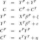
in which Y(C) is current income (consumption), divided into permanent YP(CP) and transitory YT(CT). The main objective of most papers is to estimate κ P, test whether κP > κT, and or/test whether κP = 1 (the income proportionality hypothesis). The earlier contributions (Bhalla, 1979; Musgrove, 1979) write a model for YP directly as a function of observables (such as education, occupation, industry, etc.). In contrast, Sargent (1978) and Wolpin (1982) use the restrictions on the theory imposed by the rational expectations framework. An important paper in this respect is Hall and Mishkin (1982).
4.1.1 Hall and Mishkin (1982)
The authors in the papers above do not write explicitly the stochastic structure of income. For example, in the statistical characterization above, permanent income is literally permanent (a fixed effect). The first paper to use micro panel data to decompose income shocks into permanent and transitory components writing an explicit stochastic income process is Hall and Mishkin (1982), who investigate whether households follow the rational expectations formulation of the permanent income hypothesis using PSID data on income and food consumption. Their setup assumes quadratic preferences (and hence looks at consumption and income changes), imposes that the marginal propensity to consume with respect to permanent shocks is 1, and leaves only the MPC with respect to transitory shocks free for estimation.
The income process is described by Eqs (3) and (4) (enriched to allow for some serial correlation of the MA type in the transitory component), so that the change in consumption is given by Eq. (5):
δCi,a,t = Zi,a,t + πafi,a,t.
Since the PSID has information only on food consumption, this equation is recast in terms of food spending (implicitly assuming separability between food and other non-durable goods):
![]()
where a is the proportion of income spent of food, and mF is a stochastic element added to food consumption (measurement error), not correlated with the random elements of income (ζi,a,t and εi,a,t). The model is estimated using maximum likelihood assuming that all the random elements are normally distributed.
Hall and Mishkin (1982) also allow for the possibility that the consumer has some “advance information” (relative to the econometrician) about the income process.44 Calling ϒ the degree of advance information, they rewrite their model as:
![]() (28)
(28)
Their estimates of (28) only partly confirm the PIH. Their estimate of ϒ is 0.25 and their estimate of π (which they assume to be constant over the life cycle) is 0.29, too high to be consistent with plausible interest rates. They reconcile this result with the possibility of excess sensitivity. They note that, contrary to the theory’s prediction, cov (ΔCa, ΔYa−1) = 0. Hall and Mishkin suggest a set up where a fraction μ of the households overreact to changes in transitory income rather than follow the permanent income. Estimating this model, the authors find that approximately 20 percent of consumers do not follow the permanent income hypothesis.45
4.2 Approach 2: identifying an information set for a given insurance configuration
Why can consumption and income data be useful in identifying an information set or learning more about the nature of the income process? To see this point very clearly, consider a simple extension of an example used by Browning et al. (1999). Certain features of the income process are not identifiable using income data alone. However, we might learn about them using jointly income and consumption data (or even labor supply, or more generally any choice that is affected by income). Assume that the income process is given by the sum of a random walk (pi,a,t), a transitory shock (εi,a,t) and a measurement error (mi,a,t, which may even reflect “superior information”, i.e., information that is observed by the individual but not by an econometrician):
![]()
Written in first differences, this becomes
ΔYi,a,t,= Zi,a,t + Δεi,a,t + Δmi,a,t.
As discussed in Section 3, one cannot separately identify transitory shocks and measurement error (unless access to validation data gives us an estimate of the amount of variability explained by measurement error, as in Meghir and Pistaferri, 2004; or higher order restrictions are invoked, as in Cragg, 1997; or assumptions about separate serial correlation of the two components are imposed). Assume as usual that preferences are quadratic, β (1 + r) = 1 and that the consumer’s horizon is infinite for simplicity. The change in consumption is given by Eq. (5) adapted to the infinite horizon case:
![]() (29)
(29)
The component mi,a,t does not enter (29) because consumption does not respond to measurement error in income. However, note that if raiAt represented “superior information”, then this assumption would have behavioral content: it would be violated if liquidity constraints were binding−and hence mi,a,t would belong in (29).
Suppose a researcher has access to panel data on consumption and income (a very stringent requirement, as it turns out).46 Then one can use the following covariance restrictions:
![]()
![]()
As is clear from the first two moments, ![]() and
and ![]() cannot be told apart from income data alone (although the variance of permanent shocks can actually be identified using
cannot be told apart from income data alone (although the variance of permanent shocks can actually be identified using ![]() , the stationary version of Eq. (17) above). However, the availability of consumption data solves the identification problem. In particular, one could identify the variance of transitory shocks from
, the stationary version of Eq. (17) above). However, the availability of consumption data solves the identification problem. In particular, one could identify the variance of transitory shocks from
![]() (30)
(30)
Note also that ifone is willing to use the covariance between changes in consumption and changes in income ![]() , then there is even an overidentifying restriction that can be used to test the model.
, then there is even an overidentifying restriction that can be used to test the model.
It is useful at this point to separate the literature into two sub-branches—the papers devoted to learning features of the income process, and those devoted to identifying information set.
4.2.1 Is the increase in income inequality permanent or transitory?
Blundell and Preston (1998) use the link between the income process and consumption inequality to understand the nature and causes of the increase in inequality of consumption and the relative importance of changes in the variance of transitory and permanent shocks. Their motivation is that for the UK they have only repeated cross-section data, and the variances of income shocks are changing over time due to, for example, rising inequality. Hence for a given cohort, say, and even ignoring measurement error, one has:
![]()
where j = 0 corresponds to the age of entry of this cohort in the labor market. With repeated cross-sections one can write the change in the variance of income for a given cohort as
Δvar(yi,a,t) = var(Zi,a,t) + Δvar(εi,a,t).
Hence, a rise in inequality (the left-hand side of this equation) may be due to a rise in “volatility” Δvar(εi,a,t) > 0 or the presence of a persistent income shock, var(ζi,a,t). In repeated cross-sections the problem of distinguishing between the two sources is unsolvable if one focuses just on income data. Suppose instead one has access to repeated cross-section data on consumption (which, conveniently, may or may not come from the same data set—the use of multiple data sets is possible as long as samples are drawn randomly from the same underlying population). Then we can see that the change in consumption inequality for a given cohort is:
![]()
assuming one can approximate the variance of the change by the change of the variances (see Deaton and Paxson, 1994, for a discussion of the conditions under which this approximation is acceptable). Here one can see that the growth in consumption inequality is dominated by the permanent component (for small r the second term on the right hand side vanishes). Indeed, assuming r ≈ 0, we can see that the change in consumption inequality identifies the variance of the permanent component and that the difference between the change in income inequality and the change in consumption inequality identifies the change in the variance of the transitory shock.47 However, the possibility of partial insurance, serially correlated shocks, measurement error, or lack of cross-sectional orthogonality may generate underidentification.
Related to Blundell and Preston (1998) is a paper by Hryshko (2008). He estimates jointly a consumption function (based on the CRRA specification) and an income process. Based on the evidence from Hryshko (2009) and the literature, as well as the need to match the increasing inequality of consumption over the life cycle, he assumes that the income process is the sum of a random walk and a transitory shock. However, he also allows the structural shocks (i.e. the transitory shock and the innovation to the permanent component) to be correlated. In simulations he shows that such a correlation can be very important for interpreting life cycle consumption. This additional feature cannot be identified without its implications for consumption and thus provides an excellent example of the joint identifying power of the two processes (income and consumption). He then estimates jointly the income and consumption process using simulated methods of moment. In addition, just like Blundell et al. (2008b) he estimates the proportion of the permanent and the transitory shock that are insured, finding that 37% of permanent shocks are insured via channels other than savings; transitory shocks are only insured via savings.
4.2.2 Identifying an information set
Now we discuss three examples where the idea of jointly using consumption and income data has been used to identify an individual’s information set.
Cunha et al. (2005) The authors estimate what components of measured lifetime income variability are due to uncertainty realized after their college decision time, and what components are due to heterogeneity (known at the time the decision is made). The identification strategy depends on the specification of preferences and on the assumptions made about the structure of markets. In their paper markets are complete. The goal is to identify the distributions of predictable heterogeneity and uncertainty separately. The authors find that about half of the variance of unobservable components in the returns to schooling are known and acted on by the agents when making schooling choices. The framework of their paper has been extended in Cunha and Heckman (2007), where the authors show that a large fraction of the increase in inequality in recent years is due to the increase in the variance of the unforecastable components. In particular, they estimate the fraction of future earnings that is forecastable and how this fraction has changed over time using college decision choices. For less skilled workers, roughly 60% of the increase in wage variability is due to uncertainty. For more skilled workers, only 8% of the increase in wage variability is due to uncertainty.
The following simplified example demonstrates their identification strategy in the context of consumption choices. Suppose as usual that preferences are quadratic, β (1 + r) = 1, initial assets are zero, the horizon is infinite, but the consumer receives income only in two periods, t and t + 1. Consumption is therefore
![]()
Write income in t + 1 as
![]()
where ![]() is observed by both the individual and the econometrician,
is observed by both the individual and the econometrician, ![]() is potentially observed only by the individual, and
is potentially observed only by the individual, and ![]() is unobserved by both. The idea is that one can form the following “deviation” variables
is unobserved by both. The idea is that one can form the following “deviation” variables
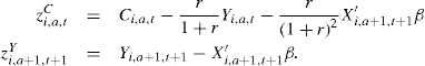
If ![]() , there is evidence of “superior information”, i.e., the consumer used more than just
, there is evidence of “superior information”, i.e., the consumer used more than just ![]() to decide how much to consume in period t.
to decide how much to consume in period t.
Primiceri and van Rens (2009) Primiceri and van Rens (2009) assume that consumers are unable to smooth permanent shocks, and that any attenuated response measures the amount of advance information that they have about developments in their (permanent) income. Using CEX data, they find that all of the increase in income inequality over the 1980–2000 period can be attributed to an increase in the variance of permanent shocks but that most of the permanent income shocks are anticipated by individuals; hence consumption inequality remains flat even though income inequality increases. While their results challenge the common view that permanent shocks were important only in the early 1980s (see Card and Di Nardo, 2002; Moffitt and Gottschalk, 1994), they could be explained by the poor quality of income data in the CEX (see Heathcote, 2009).
The authors decompose idiosyncratic changes in income into predictable and unpredictable permanent income shocks and to transitory shocks. They estimate the contribution of each element to total income inequality using CEX data. The log income process is specified as follows
![]() (31)
(31)
![]() (32)
(32)
where and ζi,a,t are ![]() unpredictable to the individual and ζi,a,t is predictable to the individual but unobservable to the econometrician. Using CRRA utility with incomplete markets (there is only a risk free bond) log consumption can be shown to follow (approximately):
unpredictable to the individual and ζi,a,t is predictable to the individual but unobservable to the econometrician. Using CRRA utility with incomplete markets (there is only a risk free bond) log consumption can be shown to follow (approximately):
![]() (33)
(33)
From Eqs (31)–(33), the following cohort-specific moment conditions are implied:
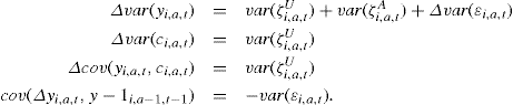
where var(.) and cov(.) denote cross-sectional variances and covariances, respectively. Using these moment conditions, it is possible to (over)identify ![]() and
and ![]() for t = 1, ..., T and var(st) for t = 0, ..., T. The authors estimate the model using a Bayesian likelihood based approach evaluating the posterior using the MCMC algorithm. They find that predictable permanent income shocks are the main source of income inequality.
for t = 1, ..., T and var(st) for t = 0, ..., T. The authors estimate the model using a Bayesian likelihood based approach evaluating the posterior using the MCMC algorithm. They find that predictable permanent income shocks are the main source of income inequality.
The model above cannot distinguish between predictable permanent shocks and risk sharing. To address this issue, the authors argue that if consumption does not respond to income shocks because of risk sharing, we would expect part of that risk sharing to happen through taxes and transfers and part through markets for financial assets. They show that re-estimating the model for income before taxes, income before taxes excluding financial income and for earned income before tax and transfers yields very close estimates to the baseline model (see Heathcote, 2009, for a discussion of their testing strategy).
Guvenen (2009) and Guvenen and Smith (2009) In Guvenen’s (2007) model, income data are generated by the heterogeneous income profile specification. However, individuals do not know the parameters of their own profile. In particular, they ignore the slope of life cycle profile fi and the value of the persistent component. They need to learn about these parameters using Bayesian updating by observing successive income realizations, which are noisy because of the mean reverting transitory shock. He shows that this model can be made to fit the consumption data very well (both in terms of levels and variance over the life cycle) and in some ways better than the process that includes a unit root. By introducing learning, Guveven relaxes the restriction linking the income process to consumption and as a result weakens the identifying information implied by this link. This allows the income process to be stationary and consumption to behave as if income is not stationary. Thus, from a welfare point of view the individual is facing essentially as much uncertainty as they would under the random walk model, which is why the model can fit the increasing inequality over the life cycle. In Guvenen’s model it is just the interpretation of the nature of uncertainty that has changed. The fact that the income process conditional on the individual is basically deterministic (except for the small transitory shock) has lost its key welfare implications. Thus whether the income is highly uncertain or deterministic becomes irrelevant for issues that have to do with insurance and precautionary savings: individuals perceive it as highly uncertain and this is all that matters.48
While Guvenen (2007) calibrates the consumption profile, Guvenen and Smith (2009) use consumption data jointly with income data to estimate the structural parameters of the model. They extend the consumption imputation procedure of Blundell et al. (2008b) to create a panel of income and consumption data in the PSID. As in Guvenen (2007), they assume that the income process is the sum of a random trend that consumers must learn about in Bayesian fashion, an AR(1) process with AR coefficient below 1, and a serially uncorrelated component.
The authors estimate the structural parameters of their model by applying an indirect inference approach—a simulation based approach suitable for models in which it is very difficult to specify the criterion function.49 The authors define an auxiliary model in which consumption and income depend on lags and leads of consumption and income, as well as growth rates of income at various lags and leads. For their estimation, the authors construct the panel of imputed household consumption by combining data from the PSID and CEX. As in Guvenen (2009) the authors find that income shocks are less persistent in the HIP case (ρ = 0.76) than in the RIP case (ρ close to one), and that there is a significant evidence for heterogeneity in income growth. In addition, they find that prior uncertainty is quite small (Λ = 0.19, meaning that about 80 percent of the uncertainty about the random trend component is resolved in the first period of life). They therefore argue that the amount of uninsurable lifetime income risk that households perceive is smaller than what is typically assumed in calibrated macroeconomic models. Statistically speaking, the estimate is very imprecise and one could conclude that everything about the random trend term is known early on in the life cycle.
4.3 Information or insurance?
In the three examples above it is possible to solve the identification problem by making the following assumptions. First, consumption responds to signal but not to noise. Similarly, consumption responds to unanticipated income changes, but not to forecastable ones. While the orthogonality of consumption to measurement error in income is not implausible, orthogonality to anticipated changes in income has behavioral content. Households will respond to anticipated changes in income, causing the theory to fail, if there are intertemporal distortions induced by, e.g. liquidity constraints.50
Second, the structure of markets is such that the econometrician can predict response of consumption to income shocks on the basis of a model of individual behavior. For example, in the strict version of the PIH with infinite horizon, the marginal propensity to consume out of a permanent shock is 1 and the marginal propensity to consume out of transitory shock is equal to the annuity value ![]() .51 That is, one identifies the variances of interest only under the assumption that the chosen model of behavior describes the data accurately.
.51 That is, one identifies the variances of interest only under the assumption that the chosen model of behavior describes the data accurately.
But what if there is more insurance than predicted by, for example, the simple PIH version of the theory? There are alternative theories that predict that consumers may insure their income shocks to a larger extent than predicted by a simple model with just self-insurance through a risk-free bond. One example is the full insurance model. Clearly, it is hard to believe full insurance is literally true. The model has obvious theoretical problems, such as private information and limited enforcement. Moreover, there are serious empirical problems: The full insurance hypothesis is soundly rejected by the data (Cochrane, 1991; Attanasio and Davis, 1996; Hayashi et al., 1996).
But outside the extreme case of the full insurance model, there is perhaps more insurance than predicted by the strict PIH version with just a risk-free bond. In Section 2.2.2, we saw that standard Bewley-type models can generate some insurance against permanent shocks as long as people accumulate some precautionary wealth. To achieve this result, one does not require sophisticated contingent Arrow-Debreu markets. All is needed is a simple storage technology (such as a saving account).
A recent macroeconomic literature has explored a number of theoretical alternatives to the insurance configurations described above. These alternative models fall under two broad groups: those that assume public information but limited enforcement of contracts, and those that assume full commitment but private information. These models prove that the self-insurance case is Pareto-inefficient even conditioning on limited enforcement and private information issues. In both types of models, agents typically achieve more insurance than under a model with a single non-contingent bond, but less than under a complete markets environment. These models show that the relationship between income shocks and consumption depends on the degree of persistence of income shocks. Alvarez and Jermann (2000), for example, explore the nature of income insurance schemes in economies where agents cannot be prevented from withdrawing participation if the loss from the accumulated future income gains they are asked to forgo becomes greater than the gains from continuing participation. Such schemes, if feasible, allow individuals to keep some of the positive shocks to their income and therefore offer only partial income insurance. If income shocks are persistent enough and agents are infinitely lived, then participation constraints become so severe that no insurance scheme is feasible. With finite lived agents, the future benefits from a positive permanent shock exceed those from a comparable transitory shock. This suggests that the degree of insurance should be allowed to differ between transitory and permanent shocks and should also be allowed to change over time and across different groups. Krueger and Perri (2006) provide an empirical review of income and consumption inequality in the 80’s and 90’s. They then suggest a theoretical macro model based on self insurance with limited commitment trying to explain the moderate expansion in consumption inequality compared to income inequality. Their hypothesis is that an increase in the volatility of idiosyncratic labor income has not only been an important factor in the increase in income inequality, but has also caused a change in the development of financial markets, allowing individual households to better insure against the bigger idiosyncratic income fluctuations.
Another reason for partial insurance is moral hazard. This is the direction taken in Attanasio and Pavoni (2007). Here the economic environment is characterized by moral hazard and hidden asset accumulation, e.g., individuals have hidden access to a simple credit market. The authors show that, depending on the cost of shirking and the persistence of the income shock, some partial insurance is possible and a linear insurance rule can be obtained as an exact (closed form) solution in a dynamic Mirrlees model with CRRA utility. In particular, the response of consumption to permanent income shocks can be interpreted as a measure of the severity of informational problems. Their empirical analysis finds evidence for “excess smoothness” of consumption with respect to permanent shocks. However, they show that the Euler equation for consumption is still valid and that the empirical content of the model lies in how consumption reacts to unexpected income shocks.
We now want to provide a simple example of the identification issue: does the attenuated response of consumption to income shocks reflect “insurance/smoothing” or “information”? Assume that log income and log consumption changes are given by the following equations:52
![]()
In this case, income shifts because of anticipated permanent changes in income (e.g., a pre-announced promotion) and unanticipated permanent changes in income. In theory, consumption changes only in response to the unanticipated component. Suppose that our objective is to estimate the extent of ”information”, i.e., how large are permanent changes in income that are unanticipated:
![]()
A possible way of identifying this parameter is to run a simple IV regression of onto Δyi,a,t using yi,a−1,t−1 + Δyi,a,t + Δyi,a+l,t+1) as an instrument (see Guiso et al., 2005). This yields indeed:
![]()
In contrast to this case, suppose now that ![]() = 0 (no advance or superior information), but there is some insurance against permanent and transitory shocks, measured by the partial insurance parameters Φ and Ψ. What is the IV regression above identifying? The model now is
= 0 (no advance or superior information), but there is some insurance against permanent and transitory shocks, measured by the partial insurance parameters Φ and Ψ. What is the IV regression above identifying? The model now is
![]() (34)
(34)
![]() (35)
(35)
and the IV parameter takes the form
![]()
which is what Blundell et al. (2008b) assume.
Hence, the same moment ![]() has two entirely different interpretations depending on what assumptions one makes about information and insurance. What if we have both an anticipated component and partial insurance? It’s easy to show that in this case
has two entirely different interpretations depending on what assumptions one makes about information and insurance. What if we have both an anticipated component and partial insurance? It’s easy to show that in this case
![]()
a combination of information and insurance.
In sum, suppose that a researcher finds that consumption responds very little to what the econometrician defines to be a shock to economic resources (for the moment, neglect the distinction between transitory and permanent shocks). There are at least two economically interesting reasons why this might be the case. First, it is possible that what the econometrician defines to be a shock is not, in fact, a shock at all when seen from the point of view of the individual. In other words, the change in economic resources identified by the econometrician as an innovation might be predicted in advance (at least partly) by the consumer. Hence if the consumer is rational and not subject to borrowing constraints, her consumption will not respond to changes in income that are anticipated. It follows that the “extent of attenuation” of consumption in response to income shocks measures the extent of ”superior information” that the consumers possess.
The other possibility is that what the econometrician defines to be a shock is correctly a shock when seen from the point of view of the individual. However, suppose that the consumer has access to insurance mechanisms over and above self-insurance (for example, government insurance, intergenerational transfers, etc.). Hence, consumption will react little to the shock (or less than predicted by a model with just self-insurance). In this case, the “extent of attenuation” of consumption in response to income shocks measures the extent of “partial insurance” that the consumer has available against income shocks.53
More broadly, identification of information sets requires taking a stand on the structure of (formal and informal) credit and insurance markets. What looks like lack of information may be liquidity constraints in disguise (consumer responds too much to negative transitory shock, and what looks like superior information may be insurance in disguise (consumer responds too little to permanent shocks).
4.4 Approaching the information/insurance conundrum
The literature has considered two approaches to solve the information/insurance identification issue. A first method attempts to identify episodes in which income changes unexpectedly, and to evaluate in a quasi-experimental setting how consumption reacts to such changes. A second approach estimates the impact of shocks combining realizations and expectations of income or consumption in surveys where data on subjective expectations are available (see Hayashi (1985) and Pistaferri (2001), for means, and Kaufmann and Pistaferri (2009), for covariance restrictions).
Each of these approaches has pros and cons, as we shall discuss below. Before discussing these approaches, we discuss Blundell et al. (2008b), which does impose assumptions about the information set(s) of the agents and estimates insurance, but provides a test of ”superior information”.
4.4.1 Blundell et al. (2008b)
The consumption model considered in Blundell et al. (2008b) is given by Eq. (12), while their income process is given by (10) and (11). In their study they create panel data on a comprehensive consumption measure for the PSID using an imputation procedure based on food demand estimates from the CEX. Table 3 reproduces their main results. They find that consumption is nearly insensitive to transitory shocks (the estimated coefficient is around 5 percent, but higher among poor households), while their estimate of the response of consumption to permanent shocks is significantly lower than 1 (around 0.65, but higher for poor or less educated households), suggesting that households are able to insure at least part of the permanent shocks.
Table 3
Partial insurance estimates from Blundell et al. (2008b).
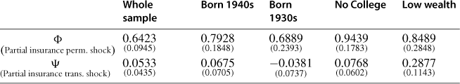
Note: Standard errors in parenthesis.
These results show (a) that the estimates of the insurance coefficients in the baseline case are statistically consistent with the values predicted by the calibrated Kaplan-Violante model of Section 2.2.2; (b) that younger cohorts have harder time smoothing their shocks, presumably because of the lack of sufficient wealth; (c) groups with actual or presumed low wealth are not able to insure permanent shocks (as expected from the model) and even have difficulties smoothing transitory shocks (credit markets can be unavailable for people with little or no collateral).
While the setting of Blundell et al. (2008b) cannot be used to distinguish between insurance and information, their paper provides a test of their assumption about richness of the information set. In particular, they follow Cunha et al. (2005) and test whether unexpected consumption growth (defined as the residual of a regression of consumption growth on observable household characteristics) is correlated with future income changes (defined also as the residual of a regression of income growth on observable household characteristics). If this was the case, then consumption contains more information than used by the econometrician. Their test of superior information reported in Table 4 shows that consumption is not correlated with future income changes.
Table 4
Test of Superior Information, from Blundell et al. (2008b).
| Test cov(Δya+l, Δca) = 0 for all a | p-value 0. 25 |
| Test cov(Δya+2, Δca) = 0 for all a | p-value 0. 27 |
| Test cov(Δya+3, Δca) = 0 for all a | p-value 0. 74 |
| Test cov(Δya+4, Δca) = 0 for all a | p-value 0. 68 |
Blundell et al. (2008b) find little evidence of anticipation. This suggests the persistent labor income shocks that were experienced in the 1980s were not anticipated. These were largely changes in the returns to skills, shifts in government transfers and the shift of risk from firms to workers.
Finally, the results of Blundell et al. (2008b) can be used to understand why consumption inequality in the US has grown less than income inequality during the past two decades. Their findings suggest that the widening gap between consumption and income inequality is due to the change in the durability of income shocks. In particular, a growth in the variance of permanent shocks in the early eighties was replaced by a continued growth in the variance of transitory income shocks in the late eighties. Since they find little evidence that the degree of insurance with respect to shocks of different durability changes over this period, it is the relative increase in the variability of more insurable shocks rather than greater insurance opportunities that explains the disjuncture between income and consumption inequality.
4.4.2 Solution 1: the quasi-experimental approach
The approach we discuss in this section does not require estimation of an income process, or even observing the individual shocks.54 Rather, it compares households that are exposed to shocks with households that are not (or the same households before and after the shock), and assumes that the difference in consumption arises from the realization of the shocks. The idea here is to identify episodes in which changes in income are unanticipated, easy to characterize (i.e., persistent or transient), and (possibly) large.
The first of such attempts dates back to a study by Bodkin (1959), who laid down fifty years ago all the ingredients of the quasi-experimental approach.55 In this pioneering study, the experiment consists of looking at the consumption behavior of WWII veterans after the receipt of unexpected dividend payments from the National Service Life Insurance. Bodkin assumes that the dividend payments are unanticipated and represent a windfall source of income, and finds a point estimate of the marginal propensity to consume non-durables out of this windfall income is as high as 0.72, a strong violation of the permanent income model.56
The subsequent literature has looked at the economic consequences of illness (Gertler and Gruber, 2002), disability (Stephens, 2001; Meyer and Mok, 2006), unemployment (Gruber, 1997; Browning and Crossley, 2001), and, in the context of developing countries, weather shocks (Wolpin, 1982; Paxson, 1992) and crop losses (Cameron and Worswick, 2003). Some of these shocks are transitory (i.e. temporary job loss), and others are permanent (disability); some are positive (dividend pay-outs), others negative (illness). The framework in Section 2 suggests that it is important to distinguish between the effects of these various types of shocks because, according to the theory, consumption should change almost one-for-one in response to permanent shocks (positive or negative), but may react asymmetrically ifshocks are transitory. Indeed, ifhouseholds are credit constrained (can save but not borrow) they will cut consumption strongly when hit by a negative transitory shock, but will not react much to a positive one.
Recent papers in the quasi-experimental framework look at the effect of unemployment shocks on consumption, and the smoothing benefits provided by unemployment insurance (UI) schemes. As pointed out by Browning and Crossley (2001) unemployment insurance provides two benefits to consumers. First, it provides “consumption smoothing benefits” for consumers who are liquidity constrained. In the absence of credit constraints, individuals who faced a negative transitory shock such as unemployment would borrow to smooth their consumption. If they are unable to borrow they would need to adjust their consumption downward considerably. Unemployment insurance provides some liquidity and hence it has positive welfare effects. Second, unemployment insurance reduces the conditional variance of consumption growth and hence the need to accumulate precautionary savings.
One of the earlier attempts to estimate the welfare effects of unemployment insurance is Gruber (1997). Using the PSID, he constructs a sample of workers who lose their job between period t − 1 and period t, and regresses the change in food spending over the same time span against the UI replacement rate an individual is eligible for (i.e., potential benefits). Gruber finds a large smoothing effect of UI, in particular that a 10 percentage point rise in the replacement rate reduces the fall in consumption upon unemployment by about 3 percent. He also finds that the fall in consumption at zero replacement rates is about 20 percent, suggesting that consumers face liquidity constraints.
Browning and Crossley (2001) extend Gruber’s idea to a different country (Canada instead of the US), using a more comprehensive measure of consumption (instead of just food) and legislated changes in UI (instead of state-time variation). Moreover, their data are rich enough to allow them to identify presumably liquidity constrained households (in particular, their data set provide information on assets at the time of job loss). Browning and Crossley estimate a small elasticity of expenditures with respect to UI benefit (5 percent). But this small effect masks substantial heterogeneity, with low-assets households at time of job loss exhibiting elasticities as high as 20 percent. This is consistent with the presence of liquidity constraints.
A critique of this approach is that the response of consumption to unemployment shocks is confounded by three sets of issues (similar arguments apply to papers that look at unpredictable income changes due to illness or disability, as in Stephens, 2001). First, some of these shocks may not come as a surprise, and individuals may have saved in their anticipation. For example, being laid off by Chrysler in 2009 should hardly come as a surprise. Ideally, one would overcome this problem by, say, matching job accident data or firm closure data with consumption data. Second, the theory predicts that consumers smooth marginal utility, not consumption per se. If an unemployment shock brings more leisure and if consumption is a substitute for leisure, an excess response of consumption to the transitory shock induced by losing one’s job does not necessarily represent a violation of the theory. Finally, even ifunemployment shocks are truly fully unanticipated, they may be partially insured through government programs such as unemployment insurance (and disability insurance in case of disability shocks). An attenuated consumption response to a permanent income shock due to disability may be explained by the availability of government-provided insurance, rather than representing a failure of the theory. Therefore a complete analysis of the impact of unemployment or disability shocks requires explicit modeling of the type of insurance available to individuals as well as of the possible interactions between public and private insurance.
The above discussion suggests that it might be easier to test the theory in contexts in which insurance over and above self-insurance is not available, such as in developing countries. Gertler and Gruber (2002) look at the effect of income shocks arising from major illness on consumption in Indonesia. They find that while people are able to smooth the effect of minor illnesses (which could be interpreted as transitory shocks, or anticipated events), they experience considerably more difficulty in smoothing the impact of major illnesses (which could be interpreted as permanent shocks).
Wolpin (1982) and Paxson (1992) study the effect of weather shocks in India and Thailand, respectively. In agricultural economies, weather shocks affect income directly through the production function and deviations from normal weather conditions are truly unanticipated events. Wolpin (1982) uses Indian regional time series data on rainfall to construct long run moments as instruments for current income (which is assumed to measure permanent income with error). The estimated permanent income elasticity ranges from 0.91 to 1.02 depending on the measure of consumption, thus supporting strongly the permanent income model. Paxson (1992) uses regional Thai data on weather to measure transitory shocks and finds that Thai consumers have a high propensity to save out of transitory weather shocks, in support of the theory. However, she also finds that they have a propensity to save out of permanent shocks above zero, which rejects a strong version of the permanent income hypothesis.
Studies using quasi-experimental variation to identify shocks to household income have the obvious advantage that the identification strategy is clear and easy to explain and understand. However, these studies’ obvious limitation is that they capture only one type of shock at a time, for instance illness, job loss, rainfall, extreme temperatures, or crop loss. One may wonder, for example, whether the Gruber (1997) and Browning and Crossley (2001) estimates obtained in a sample of job losers have external validity for examining the effect of other types of shocks (especially those that are much harder to insure, such as shocks to one’s productivity).
A second limitation of the approach is that some of the income shocks (in particular, unemployment and disability shocks), cannot be considered as truly exogenous events. For instance, for some people unemployment is a voluntary choice, and for others disability could be reported just to obtain benefits (a moral hazard issue). For this reason, not all income variability is necessarily unanticipated, or exogenous to the agent (Low et al., forthcoming). The lesson of the literature is that identifying episodes of genuine exogenous and unanticipated income changes is very difficult. One such case is weather conditions, to the extent at least to which people don’t move to different regions to offset bad weather conditions.
4.4.3 Solution 2: subjective expectations
As pointed out in Sections 4.1 and 4.2, identifying income shocks is difficult because people may have information that is not observed by the econometrician. For instance, they may know in advance that they will face a temporary change in their income (such as a seasonal lay-off). When the news is realized, the econometrician will measure as a shock what is in fact an expected event. The literature based on subjective expectations attempts to circumvent the problem by asking people to report quantitative information on their expectations, an approach forcefully endorsed by Manski (2004). This literature relies therefore on survey questions, rather than retrospective data (as in Section 4.2), to elicit information on the conditional distribution of future income, and measures shocks as deviations of actual realizations from elicited expectations.
Hayashi (1985) is the first study to adopt this approach. He uses a four-quarter panel of Japanese households containing respondents’ expectations about expenditure and income in the following quarter. Hayashi works with disaggregate consumers’ expenditure, allowing each component to have a different degree of durability. He specifies a consumption rule and, allowing for measurement error in expenditures, estimates the covariances between expected and unexpected changes in consumption and expected and unexpected changes in income. His results are in line with Hall and Mishkin (1982), suggesting a relatively high sensitivity of consumption to income shocks.
Pistaferri (2001) combines income realizations and quantitative subjective income expectations contained in the 1989–93 Italian Survey of Household Income and Wealth (SHIW) to point identify separately the transitory and the permanent income shocks. To see how subjective income expectations allow the estimation of transitory and income shocks for each household, consider the income process of Eqs (3) and (4). Define E(Xi,a,t|Ωi,a−1,t−1) as the subjective expectation of (Xi,a,t given the individual’s information set at age a − 1. It is worth pointing out that Ωi,a−1,t−1 is the set of information possessed at the individual level; the econometrician’s information set is generally less rich. The assumption of rational expectations implies that the transitory shock at time t can be point identified by:
![]() (36)
(36)
Using Eqs (3), (4) and (36), the permanent shock at time t is identified by the expression:
![]()
i. e., the income innovation at age a adjusted by a factor that takes into account the arrival of new information concerning the change in income between a and a + 1. Thus, the transitory and permanent shocks can be identified if one observes, for at least two consecutive time periods, the conditional expectation and the realization of income, a requirement satisfied by the 1989–93 SHIW Pistaferri estimates the saving for a rainy day equation of Campbell (1987) and finds that consumers save most of the transitory shocks and very little of the permanent shocks, supporting the saving for a rainy day model.
Kaufmann and Pistaferri (2009) use the same Italian survey used by Pistaferri (2001), but different years (1995–2001) to distinguish the superior information issue from the insurance issue mentioned in Section 4.2. Their empirical strategy is to consider the covariance restrictions implied by the theory on the joint behavior of consumption, income realizations, and subjective quantitative income expectations.
Their results are reproduced in Table 5. Their most general model separates transitory changes in log income into anticipated (with variance ![]() ), unanticipated
), unanticipated ![]() , and measurement error
, and measurement error ![]() ; separates permanent changes in income in anticipated
; separates permanent changes in income in anticipated ![]() and unanticipated
and unanticipated ![]() allows for measurement error in consumption and subjective income expectations (
allows for measurement error in consumption and subjective income expectations (![]() and
and ![]() , respectively), and allows for partial insurance with respect to transitory shocks (Ψ) and permanent shocks (Φ).
, respectively), and allows for partial insurance with respect to transitory shocks (Ψ) and permanent shocks (Φ).
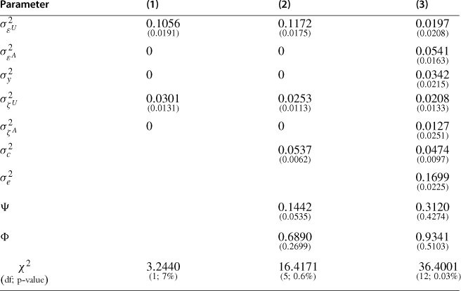
In column (1) they put themselves in the shoes of a researcher with access to just income data. This researcher cannot separate anticipated from unanticipated changes in income or transitory changes from measurement error, so she assumes that measurement error is absent and all changes are unforecastable, resulting in upward biased estimates of ![]() , and
, and ![]() ,. In column (2) they add consumption data. The researcher is still unable to separate anticipated from unanticipated, so any “superior information” is loaded onto the insurance coefficients Ψ and Φ. In particular, the data provide evidence of some insurance with respect to permanent and transitory shocks. Note that unlike what is predicted by the traditional version of the PIH, the transitory shock is not fully insured, perhaps because of binding borrowing constraints (see Jappelli and Pistaferri (2006)). In column (3) one adds data on subjective income expectations and the model is now overidentified. A number of interesting facts emerge. First, the transitory variation in income is split between the anticipated component (about 50%), the unanticipated component (20%) and measurement error (30%). This lowers the estimated degree of insurance with respect to transitory shocks. Similarly, a good fraction of the permanent variation (about 1/3) appears anticipated, and this now pushes the estimated insurance coefficient towards 1−i.e., these results show evidence that there is no insurance whatsoever with respect to permanent shocks.
,. In column (2) they add consumption data. The researcher is still unable to separate anticipated from unanticipated, so any “superior information” is loaded onto the insurance coefficients Ψ and Φ. In particular, the data provide evidence of some insurance with respect to permanent and transitory shocks. Note that unlike what is predicted by the traditional version of the PIH, the transitory shock is not fully insured, perhaps because of binding borrowing constraints (see Jappelli and Pistaferri (2006)). In column (3) one adds data on subjective income expectations and the model is now overidentified. A number of interesting facts emerge. First, the transitory variation in income is split between the anticipated component (about 50%), the unanticipated component (20%) and measurement error (30%). This lowers the estimated degree of insurance with respect to transitory shocks. Similarly, a good fraction of the permanent variation (about 1/3) appears anticipated, and this now pushes the estimated insurance coefficient towards 1−i.e., these results show evidence that there is no insurance whatsoever with respect to permanent shocks.
There are a few notes of caution to add to the commentary on these results. First, the overidentifying restrictions are rejected. Second, while the economic significance of the results is in accordance with the idea that part of the estimated smoothing effects reflect information, the standard errors are high, preventing reliable inference.
Subjective expectations: data problems
There is considerable promise in the use of subjective expectations to evaluate the validity of various consumption models. However, it is fair to say that studies that use subjective expectations are subject to various criticisms. In particular, issues are raised about their reliability and informational content; moreover, it is still the case that subjective expectations are seldom available alongside consumption and income data or are confined to special survey modules. We are aware of only four data sets containing quantitative subjective expectations of future income in developed countries: the Italian SHIW, the Dutch DHS, the Japan SFC, and the US SEE.57 See Attanasio (2009) for a survey of quantitative subjective expectation collection efforts currently undergoing in developing countries.
The Italian SHIW offers the opportunity to test some simple hypotheses regarding the validity of subjective data. In 1989 and 1991 people were asked to assign probability weights summing to 100 to various classes of income growth. In 1995 and 1998 they were asked instead to provide the minimum and maximum expected income, plus the probability that their income was going to be below the mid-point of the distribution. A first issue one may address is whether the wording of the subjective expectation questions affects reliability. The response rates for 1989, 1991, 1995 and 1998 are 57%, 96%, 87%, and 94%, respectively. The big jump in response rates between 1989 and 1991 (and somehow also between 1995 and 1998) may be due to interviewers being instructed to improve at eliciting data rather than bearing any meaningful relation with the question format. The fact that the SHIW has a panel component allows us to test for individual learning. The response rate in 1991 for people who were asked the same question format in the previous wave is 97% vs. 96% for people with no previous experience (95% vs. 95% in 1998). Hence, there is no evidence that having been asked the question before makes a difference in terms of response rates. Finally, we compute the proportions of people who are “confused”. In 1989–91 people were also asked more qualitative questions, such as whether they were expecting their income to be “rather variable” in the future. We define an individual to be “confused” if she reports income as being “rather variable” but reports a degenerate distribution of expectations. For 1995–98, we assume that an individual is confused if she reports different minimum and maximum expected incomes, but then reports a probability of income below the midpoint of zero or 100%. Although the two definitions are not strictly comparable, it is interesting that the proportion of “confused” is higher in 1989–91 (17%) than in 1995–98 (11%), suggesting that people have more difficulty understanding the first type of question (which is trying to elicit the individual p.d.f.) than the second type of question (where the goal is to elicit the individual c.d.f).
5 Income processes, labor supply and mobility
The type of income processes discussed in Section 3 do not distinguish between fluctuations in income caused by exogenous shocks and those caused by endogenous responses to shocks. This is particularly important when the income process is used to assess and simulate the amount of risk faced by individuals.
For example in all the papers considered earlier, labor supply is assumed exogenous; no attention is paid to mobility across firms; no attempt is made to understand whether a shock to productivity comes from bad health, firm re-organization, learning, changes in skill prices, etc.. In sum, this is a black box approach in which the various sources of earnings fluctuations are aggregated to form a sort of “sufficient statistic” (often due to data availability). However, one may want to analyze the economic forces behind the degree of persistence and the amount of variability we observe in earnings. One reason is that different types of shock may be differently insurable, raising important policy implications. Moreover, it may allow us to better characterize behavior.
In a key contribution in this direction Abowd and Card (1989) extended the earlier literature to consider joint movements of hours and wages. Having established that both hours and earnings growth can be represented by an MA(2) process, they then link the two based on the life cycle model. Their approach can reveal how much of the variation in earnings comes from genuine shocks to wages and how much is due to responses to these shocks through hours of work. Their conclusion was that the common components in the variation of earnings and hours could not be explained by variation in productivity. With their approach they opened up the idea of considering the stochastic properties of different related quantities jointly and using this framework to assess how much of the fluctuations can be attributed to risk, as opposed to endogenous response, such as changing hours. Ofcourse, to the extent that hours may be driven by short term demand for labor in the workplace, rather than voluntary adjustments, such fluctuations may also represent risk.
Extending the income process to allow for endogenous fluctuations
The key issue highlighted by the Abowd and Card approach is the distinction between shocks and responses to shocks. While Abowd and Card do not go all the way in that direction, they do relate the fluctuations in earnings and hours.
Low et al. (forthcoming) develop this direction by taking a much more structural approach and explicitly modeling labor supply and job mobility in a search and matching framework.58 Not only is this approach explicit about distinguishing between shocks and responses to shocks, but it also distinguishes different types of uncertainty, loosely associated with employment risk and productivity risk.
The first important modification is Low et al. (forthcoming) they are now explicit about modeling wages per unit of time. In the specific application the unit of time is a quarter and the individual may either be working over this period or not. Extending the framework to a richer labor supply framework (the intensive margin) is relatively straightforward. The second modification is allowing for match effects; this implies that one source of fluctuations is obtaining a different job; what job one samples is a separate source of risk, to the extent that match effects are important. However, individuals can accept or reject job offers, a fact that needs to be recognized when combining such a process with a model of life cycle consumption and labor supply.
In what follows we use the notation w for (hourly) wages. Hence we specify
![]() (37)
(37)
where Wi,a,t is the real hourly wage, dt represents the log price of human capital at time t, Xi,a,t a vector of regressors including age, pi,a,t the permanent component of wages, and the transitory error component. All parameters of the wage process are education specific (subscripts omitted for simplicity).
In principle, the term ei,a,t might be thought of as representing a mix between a transitory shock and measurement error. In the usual decomposition of shocks into transitory and permanent components, researchers work with annual earnings data where transitory shocks may well be important because of unemployment spells. In this framework, what is probably the most important source of transitory shocks is modeled explicitly through the employment and job mobility.
The term aij(t0) denotes a firm-worker match-specific component where j (t0) indexes the firm that the worker joined in period t0 ≤ t.59 It is drawn from a normal distribution with mean zero and variance ![]() . Low et al. (forthcoming) model the match effect as constant over the life of the worker-employer relationship. If the worker switches to a different employer between t and t + 1, however, there will be some resulting wage growth which we can term a mobility premium denoted as ξi,a+1,t+1 = aij(t+1) − aij (t0). The match effect is assumed normally distributed and successive draws of aij (t) are assumed independent; however, because of the endogenous mobility decisions successive realizations of the match effect will be correlated. Since offers can be rejected when received, only a censored distribution of ξa+1,t+1 is observed. The match effect aij(.) is complementary to individual productivity.60 Both the match effect and the idiosyncratic shock can have education-specific distributions. To keep things relatively simple, suppose the information structure is such that workers and firms are completely informed about ui,a,t and aij (.) when they meet (jobs are “search goods”).61
. Low et al. (forthcoming) model the match effect as constant over the life of the worker-employer relationship. If the worker switches to a different employer between t and t + 1, however, there will be some resulting wage growth which we can term a mobility premium denoted as ξi,a+1,t+1 = aij(t+1) − aij (t0). The match effect is assumed normally distributed and successive draws of aij (t) are assumed independent; however, because of the endogenous mobility decisions successive realizations of the match effect will be correlated. Since offers can be rejected when received, only a censored distribution of ξa+1,t+1 is observed. The match effect aij(.) is complementary to individual productivity.60 Both the match effect and the idiosyncratic shock can have education-specific distributions. To keep things relatively simple, suppose the information structure is such that workers and firms are completely informed about ui,a,t and aij (.) when they meet (jobs are “search goods”).61
Assume that the permanent component of wages follows a random walk process:
![]() (38)
(38)
The random shock to the permanent process, ξi,a,t is normally distributed with mean zero and variance ![]() and is independent over time. Assume this shock reflects uncertainty.62
and is independent over time. Assume this shock reflects uncertainty.62
Given a particular level of unobserved productivity, the worker will be willing to work for some firms but not for others, depending on the value of the match. The measurement error ei,a,t is normally distributed with variance ![]() and independent over time. As far as the policy implications of the model are concerned, we are interested in estimating
and independent over time. As far as the policy implications of the model are concerned, we are interested in estimating ![]() and
and ![]() . We describe later how these are estimated.
. We describe later how these are estimated.
In order to make sense of such a process, we need to make further assumptions relating to firm behavior. Thus it is simpler to assume that there are constant returns to scale in labor implying that the firm is willing to hire anyone who can produce non-negative rents. In this context, receiving an outside offer is akin to a wage shock; however, a worker need not accept such an outside offer. This means that some wage rises, that are due to such offers are attributed to pure risk. In practice they are the result of a shock and a response to that shock. The implicit assumption is that the firm does not respond to outside offers.63
The above structure describes both the sources of shocks and the reactions to them. First, we have the shocks to productivity ξi,a,t; second, there are shocks to job opportunities: these are reflected in the job arrival rate when employed and when unemployed, as well as by the possibility of a lay off (job destruction). Finally, there is the draw of a match specific effect. Individuals can respond to these by quitting into unemployment and accepting or rejecting a job offer. This model clarifies what aspect of earnings fluctuations reflects risk and what reflects an endogenous reaction to risk. The discussion also highlights the distinction between just describing the fluctuations of income vis-a-vis estimating a model of income fluctuations whose intention is to understand the welfare implications of risk.
Estimating the model Once we recognize that earnings fluctuations are also due to endogenous reactions to shocks, we need to take this into account in estimation in an internally consistent way. In the Low et al. (forthcoming) model the two ways that individuals can react is by deciding whether to work or not and deciding whether to accept alternative job offers. These decisions are a function of the offers received by the worker, which means that the distribution of wages is truncated both by the decision to work or not and by the decision to move firms. Thus estimating the components of risk involves correcting for selection both into work and for job mobility.
The effect of the modifications that Low et al. (forthcoming) allow for relative to the standard approach, and in particular that of accounting for the effect of job mobility, is to reduce substantially the estimated variance of permanent shocks from the one reported in, for example, Meghir and Pistaferri (2004). However, this does not necessarily mean that overall uncertainty declined: these modifications have changed the balance between permanent and transitory factors and have allowed for a better understanding of the sources of uncertainty and its welfare implications. Job destruction for example is a transitory, albeit persistent shock, because after a while it is expected that the individual will obtain a job and climb again the ladder of job quality. Persistence will be governed by the rate of arrival of job offers. On the other hand shocks to wages are literally permanent because of the random walk structure. The authors show that data simulated from the model can indeed replicate very well the earnings dynamics estimated with the less structural approaches in the literature. The differences in modeling are however very important because they have implications for consumption, savings and welfare.
The second recent paper along the lines of understanding the sources of shocks is that of Altonji et al. (2009). They estimate a complex stochastic model of wages, hours of work, transitions between employment and unemployment, and between jobs. Each of these events is governed by a reduced form model depending on exogenous characteristics, endogenous states and on exogenous shocks, which are the underlying source of fluctuations. Importantly, the model allows for selection into work and selection induced by transitions between jobs. The stochastic process of wages includes a match specific effect, an individual fixed effect and an AR(1) process; the AR coefficient is estimated to be 0.92 in various specifications, which is short of a random walk. Persistence is further reinforced by an AR(1) transitory shock and a further independent shock to earnings, which follows an AR process with an estimated coefficient of about 0.55. The lack of a random walk and the overall structure of the model does mean that the fit of the standard deviation of log earnings is not very good. In particular, the model predicts a flatter life cycle profile in the cross sectional variance of log-earnings than what is seen in the data. Nevertheless, both these papers make it clear that in order to understand uncertainty and its impact we need to account for the origin of the shocks. This should help further in identifying the nature of uncertainty and the persistence of shocks.
Other approaches to endogenizing volatility
Here we discuss other approaches to endogenizing wage or earnings volatility.
Postel-Vinay and Turon (2010) test whether the observed covariance structure of earnings in the UK may be generated by a structural job search model with on-the-job search. Individuals who are currently unemployed can move back into employment conditional on receiving an offer and finding this offer acceptable; people with jobs can stay with their current employer (if the job is not destroyed), move to another firm (conditional on receiving an outside offer) or move into unemployment. In each period, offered wages are subject to i.i.d. productivity shocks. These may induce renegotiations (by mutual consent) of the bargained wage, resulting occasionally in wage cuts or wage raises. However, mutual consent means that there are cases in which productivity shocks are insufficient to generate wage changes, and so wages are fixed at the previous period’s level. This is the primary source of persistence observed in the data—an analyst may find evidence of a random walk in earnings even though the underlying productivity shock to wages is a pure i.i.d.
Low and Pistaferri (2010) use data on subjective reports of work limitations available from the PSID to identify health shocks separately from other shocks to productivity. Their framework is similar to that of Low et al. (forthcoming). It is simpler in certain dimensions (there are no firm specific effects and hence no job-to-job decisions), but richer in others (the modeling of health risk, the disability insurance institutional framework and the behavior of the social security system in the screening process). They use their model to assess quantitatively how large are the screening errors made by the disability evaluators and to examine the welfare consequences of changes in the features of the disability insurance program that affect the insurance-incentive trade-off, such as increasing the strictness of the screening test, reducing benefits, or increasing the probability of re-assessment.
Huggett et al. (2009) study human capital accumulation. In their model individuals may choose to divert some of their working time to the production of human capital. People differ in initial human capital (schooling, parents’ teachings, etc.), initial financial wealth, and the innate ability to learn. Among other things, their framework generalizes Ben-Porath (1967) to allow for risk, i.e., shocks to the existing stock of human capital. Their questions of interest are: (a) How much of lifetime inequality is determined before entry in the labor market (initial conditions)? and (b) How much is due to episodes of good or bad luck over the life cycle (shocks)? The answers to these two questions have clear policy relevance. Ifthe answer to (a) is “a lot”, one would want early intervention policies (e.g., public education). If the answer to (b) is “a lot”, one would want to expand income maintenance programs (UI, means-tested welfare, etc.). In Huggett et al. (2009) wages grow because of shocks to existing human capital, or systematic fanning out due to differences in learning abilities. Old people do not invest, hence only the first force is present at the end of the life cycle. This provides an important idea for identification: Data on old workers can be used to identify the distribution of shocks to human capital. They next construct an age profile for the first, second, and third moment of earnings. Age, time, and cohort effects are not separately identifiable, so need to impose some restrictions, such as: (a) No time effects, or (b) No cohort effects. Finally, they calibrate the distribution of initial conditions (initial human capital and learning ability) and the shape of the human capital production function to match the age profile of the first three moments of earnings, while fixing the remaining parameters to realistic values taken from the literature. Huggett et al. (2009) use their model to do two things: (1) compute how much lifetime inequality is due to initial conditions and how much is due to shocks, and (2) run counterfactual experiments (shutting down risk to human capital or learning ability differences). Their results are that between 60% and 70% of the variability in lifetime utility (or earnings) is due to variability in initial conditions. Among initial conditions, the lion’s share is taken by heterogeneity in initial human capital (rather than initial wealth or innate ability). Eliminating learning ability heterogeneity makes the age profile of inequality flat (even declining over a good fraction of the working life, 35–55). Eliminating shocks to human capital generates a more moderate U-shape age profile of inequality. For our purposes, one of the main points of the paper is that the standard incomplete markets model (for example, Heathcote (2009))—which assumes an exogenous income process—may exaggerate the weight played by shocks as opposed to initial conditions in determining lifetime inequality. Hence, it may overestimate the welfare gain of government insurance programs and underestimate the welfare gain of providing insurance against “bad initial conditions” (bad schools, bad parents, bad friends, etc.). Note however that the “exaggeration” effect of incomplete markets models only holds under the assumption that initial conditions are fully known to the agents at the beginning of the life cycle. Ifpeople have to “learn” their initial conditions, then they will face unpredictable innovations to these processes. Recent work by Guvenen (2007) estimates that people can forecast only about 60% of their “learning ability”—the remaining 40% is uncertainty revealed (quite slowly) over the life cycle. Similar conclusions are reached in work by Cunha et al. (2005).
Shocks and labor market equilibrium
We have moved from the standard reduced form models of income fluctuations to the more structural approach of Low et al. (forthcoming). However, there is further to go. What is missing from this framework is an explicit treatment of equilibrium pay policies. More specifically, in Low et al. (forthcoming) the wage shocks are specified as shocks to the match specific effect, without specifying how these shocks arise. If we think about the match specific effect as being produced by a combination of the qualities of the worker and of the firm, then as in Postel-Vinay and Robin (2002), we can work out the pay policy of the firm under different assumptions on the strategies that individuals and firms follow. In that framework income/earnings, but only because individuals either receive alternative job offers, to which the incumbent firm responds, or because they move to an alternative firm.
Lise et al. (2009) generalize this framework to allow for shocks to the firm’s productivity. In this context, the observed wage shocks are further decomposed into fluctuations originating in shocks to the productivity of the firm, responses to alternative offers or to moving to new jobs, either via unemployment or directly by firm to firm transition. In this context, the shocks are specified as changes in basic underlying characteristics of the firm as well as due to search frictions. This model thus comes closest to providing a full structural interpretation of income shocks, allowing also for the behavior of firms and strategies that lead to wages not being always responsive to the underlying shocks.64 While this offers a way forward in understanding the source of fluctuations, the approach is not complete because it assumes that both individuals and firms are risk neutral. In this sense individuals have no interest in insurance and do not save for precautionary reasons. Extending such models to allow for risk aversion, wage contracts that partially insure the worker and for savings, is the natural direction for obtaining an integrated approach of earnings fluctuations and an analysis of the effects of risk.65
To provide an idea of how these more structural approaches work, we give a brief overview of the Lise et al. (2009) model. Individuals are characterized by a type denoted by x. These are individual characteristics that are possibly observed or unobserved. The key restriction here is that all characteristics contribute to one productivity index. Individual utility is the income they receive from work, as in a standard search model. This linearity is technically very important but as said above it precludes any consideration of risk aversion. A key ingredient in the Lise et al. (2009) paper is that firms or jobs employ one worker in a particular position, which is an extreme form of decreasing returns to scale and leads to an option value of waiting for a good worker under certain circumstances. The job is also characterized by a type y; this can be thought of as representing prior investments in technology and market conditions. However, this productivity level is subject to shocks, which can be conceived of as product market shocks. A key ingredient of the model is that the individual characteristics and the firm type may be complementary, in such a way that total output in the economy can be increased by allocating good worker types to high productivity firms and lower worker types to lower productivity ones (log-super modularity), very much like in a Becker marriage market.
At the heart of the model is pay determination in response to the quality of the worker and the firm, and in response to outside offers that result from on-the-job search. Very much like Low et al. (forthcoming), the following shocks are embedded in the model: random changes in productivity y, individuals receiving an outside offer from an alternative job, and exogenous job destruction. However, the important difference is that Lise et al. (2009) derive the impact of these shocks to both employment and wages explicitly accounting for the incentive structure both from the side of the worker and the firm making persistence endogenous. Specifically, when the productivity of the firm changes, this translates to a wage change only if the relationship remains profitable and one of the two partners can make a credible threat to leave the partnership; if the relationship ceases to be feasible there is separation; and if there is no common agreement to renegotiate, wages remain at their previous level. The model leads to a number of inter-esting implications about the stochastic evolution of wages and about pay policy: wages are smoother than productivity; the effect of worker and firm heterogeneity cannot be decomposed in a log-linear fashion as in Abowd et al. (1999); and wages grow with time, due to on the job search. It is possible that the combination of the relatively smooth pay policy within the firm and the nature of job mobility combine to give a time series process of wages that looks like a random walk, as discussed by Postel-Vinay and Turon (2010): In their model the combination of i.i.d. shocks and wage renegotiations in an environment with search frictions leads to wages with a unit root. Interestingly they also show that the implied variance of the shocks can have an ARCH structure, as identified by Meghir and Pistaferri (2004).
6 Conclusions
We started this chapter by discussing the importance of measuring and understanding labor market risks. In particular, what is the impact of risk on behavior? What types of risks matter? Answering these questions has proved to be quite difficult. One banal problem that hinders analysis is that for the countries most studied in the literature, the US and the UK, long panel data with regular observations on consumption, income and wealth are not available. Moreover, in most cases data are of debatable quality. Take the issue of answering the question whether the rise in inequality is due to phenomena like skill-biased technical change or wage instability. One proposal (as argued in Blundell and Preston, 1998) is to study consumption inequality. The papers that have done so include Cutler and Katz (1992), Dynarski and Gruber (1997), Krueger and Perri (2006), Blundell et al. (2008b), and Attanasio et al. (2004). Most papers find that consumption inequality rises less than income inequality. In the US the difference is substantial, and some papers go so far as to claim that consumption inequality has not changed at all (Krueger and Perri). Given that all these analyses use the CEX, and given that the CEX suffers from severe problems of detachment from National Accounts, it is worth wondering whether this evidence is spurious and due to data problems.66 Some recent papers (Attanasio et al., 2004; Battistin and Padula, 2010), have combined Diary and Interview CEX data in an ingenious way to revise upward the estimates of the trends in consumption inequality. Nevertheless, the finding that consumption inequality rises less rapidly than income inequality is confirmed.
We have discussed how empirical researchers have come up with ingenious ways of remedying data difficulties. A separate problem is that identification of the “correct” income process from income data is not straightforward. Yet, the income process is key for interpreting and predicting consumption responses. For example, the theory predicts that consumption responds strongly to permanent shocks and very little to transitory shocks. But we do not observe these components separately, so we have to come up with methods (typically, statistical methods) to extract them from observed income data. These methods may suffer from bias or statistical power problems. Furthermore, even if repeated observations of income realizations were able to provide information on the “correct” income process (in terms of its persistence, number of components, etc.), it would still not solve the problem of how much of the measured variability is anticipated and how much is unanticipated by the consumer, which is another key distinction for predicting consumption responses to changes in income. As said earlier, the theory predicts that consumption responds to unanticipated changes but not to anticipated ones (unless there are liquidity constraints or adjustment costs). In the literature, authors have suggested that some of these problems can be solved by the joint use of consumption and income data (or labor supply and income data). While this is an important development, it does not necessarily solve the problem. There is a third distinction (besides “permanent vs. transitory” and “anticipated vs. unanticipated”) that is necessary to understand how consumption reacts to shocks; the distinction between “insurable” and “uninsurable” (or partially insurable) shocks, which requires taking some stand on such complicated issues as structure of credit and insurance markets, other decision margins within the household (spousal labor supply, family networks, etc.), and the modeling of government transfers (which may sometimes displace private transfers and self-insurance). This is an identification problem that has so far found only partial and unsatisfactory solutions.
Finally, on the data front one has to point out that large progress has been achieved through the use of administrative data available now in many countries. This of course does not solve the problems with consumption data, but it does allow us to understand potentially much better the dynamics of income and of wage determination. Much can be achieved by further theoretical developments and the systematic collection of excellent data.
References
1. Abowd John, Card David. On the covariance structure of earnings and hours changes. Econometrica. 1989;57(2):411–445.
2. Abowd John, Kramarz Francis, Margolis David. High wage workers and high wage firms. Econometrica. 1999;67(2):251–333.
3. Acemoglu Daron, Pischke Jorn-Steffen. Why do firms train? Theory and evidence. Quarterly Journal of Economics. 1998;113(1):79–118.
4. Altonji Joseph, Paula Martins Ana, Siow Aloysious. Dynamic factor models of consumption, hours, and income. Research in Economics. 2002;56(1):3–59.
5. Altonji Joseph, Williams Nicholas. Do wages rise with job seniority? A reassessment. Industrial and Labor Relations Review. 2005;58(3):370–397.
6. Altonji Joseph, Smith Anthony, Vidangos Ivan. Modeling earnings dynamics Finance and economics dicussion series. Washington, DC: Federal Reserve Board, Divisions of Research & Statistics and Monetary Affairs; 2009.
7. Alvarez Fernando, Jermann Urban. Efficiency, equilibrium and asset pricing with risk of default. Econometrica. 2000;68(4):775–797.
8. Alvarez J. Dynamics and seasonality in quarterly panel data: an analysis of earnings mobility in Spain. Journal of Business and Economic Statistics. 2004;22(4):443–456.
9. Angelucci, Manuela, De Giorgi, Giacomo, Rangel, Marcos, Rasul, Imran, 2010. Insurance and investment within family networks.
10. Attanasio Orazio. Expectations and perceptions in developing countries: Their measurement and their use. American Economic Review. 2009;99(2):87–92.
11. Attanasio Davis Steven J. Relative wage movements and the distribution of consumption. Journal of Political Economy. 1996;104(6):1227–1262.
12. Attanasio Orazio, Low Hamish. Estimating Euler equations. Review of Economic Dynamics. 2004;7(2):406–435.
13. Attanasio, O. P., Pavoni, N., 2007. Risk sharing in private information models with asset accumulation: explaining the excess smoothness of consumption. NBER Working Paper 12994.
14. Attanasio OP, Weber G. Consumption and saving: models of intertemporal allocation and their implications for public policy. University College London: Mimeo; 2010.
15. Attanasio, Orazio, Battistin, Erich, Ichimura, Hidehiko, 2004. What really happened to consumption inequality in the US? NBER Working Paper 10338.
16. Attanasio Orazio, Low Hamish, Sanchez-Marcos Virginia. Explaining changes in female labor supply in a life-cycle model. American Economic Review. 2008;98(4):1517–1552.
17. Attfield Clifford LF. Estimation of the structural parameters in a permanent income model. Economica. 1976;43(171):247–254.
18. Attfield Clifford LF. Testing the assumptions of the permanent-income model. Journal of the American Statistical Association. 1980;75(369):32–38.
19. Azariadis Costas. Implicit contracts and underemployment equilibria. Journal of Political Economy. 1975;83(6):1183–1202.
20. Baily Martin N. On the theory of layoffs and unemployment. Econometrica. 1977;45(5):1043–1063.
21. Baker Michael. Growth-rate heterogeneity and the covariance structure of life-cycle earnings. Journal of Labor Economics. 1997;15(2):338–375.
22. Baker Michael, Solon Gary. Earnings dynamics and inequality among Canadian Men, 1976–1992: evidence from longitudinal income tax records. Journal of Labor Economics. 2003;21(2):267–288.
23. Banks James, Blundell Richard, Brugiavini Agar. Risk pooling, precautionary saving and consumption growth. Review of Economic Studies. 2001;68(4):757–779.
24. Barsky Robert, Thomas Juster F, Kimball Miles S, Shapiro Matthew D. Preference parameters and behavioral heterogeneity: an experimental approach in the health and retirement study. Quarterly Journal of Economics. 1997;112(2):537–579.
25. Battistin Erich, Blundell Richard, Lewbel Arthur. Why is consumption more log normal than income? Gibrat’s law revisited. Journal of Political Economy. 2009;117(6):1140–1154.
26. Battistin, Erich, Padula, Mario, 2010. Errors in survey reports of consumption expenditures. Unpublished manuscript.
27. Beegle Kathleen, Thomas Duncan, Frankenberg Elizabeth, Sikoki Bondan, Strauss John, Teruel Graciela. Education during a crisis. Journal of Development Economics. 2004;74(1):53–86.
28. Besley Timothy. Savings, credit and insurance. In: Chenery Hollis, Srinivasan TN, eds. Handbook of Development Economics. Elsevier 1995;2123–2207. vol. 3. (Chapter 36).
29. Ben-Porath Yoram. The production of human capital and the life cycle of earnings. Journal of Political Economy. 1967;75(4):352–365.
30. Bertola Giuseppe, Guiso Luigi, Pistaferri Luigi. Uncertainty and consumer durables adjustment. Review of Economic Studies. 2005;72(4):973–1007.
31. Bhalla Surjit S. Measurement errors and the permanent income hypothesis: evidence from rural India. American Economic Review. 1979;69(3):295–307.
32. Blanchard Olivier J, Katz Lawrence F. Regional evolutions. Brookings papers on Economic Activity. 1992;1:1–61.
33. Blanchard Olivier Jean, Mankiw Gregory N. Consumption: beyond certainty equivalence. American Economic Review. 1988;78(2):173–177.
34. Blundell Richard, Pistaferri Luigi. Income volatility and household consumption: the impact of food assistance programs. Journal of Human Resources. 2003;38(Supplement):1032–1050.
35. Blundell Richard, Preston Ian. Consumption inequality and income uncertainty. Quarterly Journal of Economics. 1998;113(2):603–640.
36. Blundell Richard, Stoker Thomas. Consumption and the timing of income risk IFS Working Papers: W94/09. London: Institute for Fiscal Studies; 1994.
37. Blundell Richard, Low Hamish, Preston Ian. Decomposing changes in income risk using consumption data IFS Working Papers: W08/13. London: Institute for Fiscal Studies; 2008a.
38. Blundell Richard, Pistaferri Luigi, Preston Ian. Consumption inequality and partial insurance. American Economic Review. 2008b;98(5):1887–1921.
39. Bodkin R. Windfall income and consumption. American Economic Review. 1959;49(4):602–614.
40. Bohlmark Anders, Lindquist Matthew J. Life-cycle variations in the association between current and lifetime income: replication and extension for Sweden. Journal of Labor Economics. 2006;24(4):879–896.
41. Bound John, Krueger Alan. The extent of measurement error in longitudinal earnings data: do two wrongs make a right? Journal of Labor Economics. 1991;9(1):1–24.
42. Bound John, Brown Charles, Duncan Greg, Rodgers Wilalrd. Evidence on the validity of cross-sectional and longitudinal labor market data. Journal of Labor Economics. 1994;12(3):345–368.
43. Bound John, Brown Charles, Mathiowetz Nancy. Measurement error in survey data. In: Handbook of Econometrics. North-Holland, Amsterdam, New York, Oxford: Elsevier Science; 2001; vol. 5 (Chapter 59).
44. Browning Martin, Crossley Thomas. Unemployment insurance benefit levels and consumption changes. Journal of Public Economics. 2001;80(1):1–23.
45. Browning, Martin, Crossley, Thomas, 2003. Shocks, stocks and socks: consumption smoothing and the replacement of durables. Working Paper 2003–07, McMaster University Department of Economics.
46. Browning Martin, Lusardi Annamaria. Household saving: micro theories and micro facts. Journal of Economic Literature. 1996;34(4):1797–1855.
47. Browning Martin, Ejrnaes Mette, Alvarez Javier. Modelling income processes with lots of heterogeneity Discussion Paper 285. Oxford, UK: University of Oxford Department of Economics; 2006.
48. Browning Martin, Peter Hansen Lars, Heckman James. Micro data and general equilibrium models. In: Handbook of Macroeconomics. North-Holland, Amsterdam, New York, Oxford: Elsevier Science; 1999;543–633. vol. 1A.
49. Caballero Ricardo. Consumption puzzles and precautionary savings. Journal of Monetary Economics. 1990;25(1):113–136.
50. Cahuc Pierre, Postel-Vinay Fabien, Robin Jean-Marc. Wage bargaining with on-the-job search: theory and evidence. Econometrica. 2006;74(2):323–364.
51. Cameron Lisa, Worswick Christopher. The labor market as a smoothing device: labor supply responses to crop loss. Review of Development Economics. 2003;7(2):327–341.
52. Campbell JY. Does saving anticipate declining labor income? An alternative test of the permanent income hypothesis. Econometrica. 1987;55:1249–1273.
53. Cappellari L. The dynamics and inequality of Italian men’s earnings: long-term changes or transitory fluctuations? Journal of Human Resources. 2004;XXXIX(2):475–499.
54. Card D, Di Nardo JE. Skill-biased technological change and rising wage inequality: some problems and puzzles. Journal of Labor Economics. 2002;20(4):733–783.
55. Carroll, Christopher, 2001. Precautionary saving and the marginal propensity to consume out of permanent income. NBER Working Paper 8233.
56. Carroll Christopher D, Kimball Miles S. Liquidity constraints and precautionary saving. Johns Hopkins University: Manuscript; 2005.
57. Carroll Christopher, Samwick Andrew. How important is precautionary saving? Review of Economics and Statistics. 1998;80(3):410–419.
58. Chamberlain, Gary, Hirano, Keisuke, 1999. Predictive distributions based on longitudinal earnings data. Annales d’Economie et de Statistique 55–56, 211–242.
59. Chao HK. Milton Friedman and the emergence of the permanent income hypothesis. History of Political Economy. 2003;35(1):77–104.
60. Chetty Raj, Szeidl Adam. Consumption commitments and risk preferences. The Quarterly Journal of Economics. 2007;122(2):831–877.
61. Cochrane John. A simple test of consumption insurance. Journal of Political Economy. 1991;99(5):957–976.
62. Cragg JG. Using higher moments to estimate the simple errors-in-variables model. Rand Journal of Economics. 1997;28(0):S71–S91.
63. Cunha, Flavio, Heckman, James, 2007. The evolution of inequality, heterogeneity and uncertainty in labor earnings in the US Economy. IZA Discussion Paper No. 3115.
64. Cunha Flavio, Heckman James, Navarro Salvador. Separating uncertainty from heterogeneity in life cycle earnings. Oxford Economic Papers. 2005;57(2):191–261.
65. Cutler David, Katz Lawrence. Rising inequality? Changes in the distribution of income and consumption in the 1980’s. American Economic Review, Papers and Proceedings. 1992;82(2):546–551.
66. Davis, Steven, Willen, Paul, 2000. Occupation-level income shocks and asset returns: their covariance and implications for portfolio choice. CRSP Working Paper No. 523.
67. Deaton Angus, Paxson Christina. Intertemporal choice and inequality. Journal of Political Economy. 1994;102(3):384–394.
68. Dehejia Rajeev, DeLeire Thomas, Luttmer Erzo. Insuring consumption and happiness through religious organizations. Journal of Public Economics. 2007;91(1–2):259–279.
69. Dickens Richard. The evolution of individual male earnings in Great Britain: 1975–95. The Economic Journal. 2000;110(460):27–49.
70. Dominitz Jeff, Manski Charles. Using expectations data to study subjective income expectations. Journal of the American Statistical Association. 1997;92(439):855–867.
71. Dynarski Susan, Gruber Jonathan. Can families smooth variable earnings? Brooking Papers on Economic Activity. 1997;1:229–305.
72. The Economist, 2007. Shifting Sand. January 6: 63.
73. Farber Henry, Gibbons Robert. Learning and wage dynamics. Quarterly Journal of Economics. 1996;111(4):1007–1047.
74. Friedman M. A Theory of the Consumption Function. Princeton: Princeton University Press; 1957.
75. Fuchs-Schundeln Nicola, Schundeln Matthias. Precautionary savings and self-selection: evidence from the German reunification ‘experiment’. Quarterly Journal of Economics. 2005;120(3):1085–1120.
76. Gertler P, Gruber J. Insuring consumption against illness. American Economic Review. 2002;92(1):51–70.
77. Geweke John, Keane Michael. An empirical analysis of earnings dynamics among men in the PSID: 1968–1989. Journal of Econometrics. 2000;96(2):293–356.
78. Ginja Rita. Income shocks and investments in human capital. University College London Department of Economics: Mimeo; 2010.
79. Gollier C, Pratt JW. Risk vulnerability and the tempering effect of background risk. Econometrica. 1996;64(5):1109–1123.
80. Gorodnichenko Yuriy, Stolyarov Dmitriy, Sabirianova Klara. Inequality and volatility moderation in Russia: evidence from micro-level panel data on consumption and income. Review of Economic Dynamics. 2010;13:209–237.
81. Gottschalk, Peter, Moffitt, Robert, 1995. Trends in the covariance structure of earnings in the US: 1969–1987. Working Paper, Boston College Department of Economics.
82. Gruber J. The consumption smoothing benefits of unemployment insurance. American Economic Review. 1997;87(1):192–205.
83. Gruber Jonathan, Yelowitz Aaron. Public health insurance and private savings. Journal of Political Economy. 1999;107(6):1249–1274.
84. Guiso Luigi, Jappelli Tullio, Pistaferri Luigi. An empirical analysis of earnings and employment risk. Journal of Business and Economic Statistics. 2002;20(2):241–253.
85. Guiso Luigi, Jappelli Tullio, Terlizzese Daniele. Earnings uncertainty and precautionary saving. Journal of Monetary Economics. 1992;30(2):307–337.
86. Guiso Luigi, Jappelli Tullio, Terlizzese Daniele. Income risk, borrowing constraints, and portfolio choice. American Economic Review. 1996;86(1):158–172.
87. Guiso Luigi, Pistaferri Luigi, Schivardi Fabiano. Insurance within the firm. Journal of Political Economy. 2005;113(5):1054–1087.
88. Guvenen Fatih. Learning your earning: are labor income shocks really very persistent? American Economic Review. 2007;97(3):687–712.
89. Guvenen Fatih. An empirical investigation of labor income processes. Review of Economic Dynamics. 2009;12:58–79.
90. Guvenen Fatih, Smith Anthony. Inferring labor income risk from economic choices: an indirect inference approach. University of Minnesota: Mimeo; 2009.
91. Hacker Jacob. The Great Risk Shift: the Assault on American Jobs, Families, Health Care, and Retirement and How You Can Fight Back. New York: Oxford University Press US; 2006.
92. Haider Stephen, Solon Gary. Life-cycle variation in the association between current and lifetime earnings. American Economic Review. 2006;96(4):1308–1320.
93. Hall RE. Stochastic implications of the life-cycle permanent income hypothesis: theory and evidence. Journal of Political Economy. 1978;86:971–987.
94. Hall RE, Mishkin FS. The sensitivity of consumption to transitory income: estimates from panel data on households. Econometrica. 1982;50:461–481.
95. Hause John. The fine structure of earnings and the on-the-job training hypothesis. Econometrica. 1980;48(4):1013–1029.
96. Hayashi F. The permanent income hypothesis and consumption durability: analysis based on Japanese panel data. Quarterly Journal of Economics. 1985;100:1083–1113.
97. Hayashi Fumio, Altonji Joseph, Kotlikoff Lawrence. Risk sharing between and within families. Econometrica. 1996;64(2):261–294.
98. Heathcote Jonathan. Discussion of Heterogeneous Life-Cycle Profiles, Income Risk and Consumption Inequality by Giorgio Primiceri and Thijs van Rens. Journal of Monetary Economics. 2009;56(1):40–42.
99. Heathcote, Jonathan, Storesletten, Kjetil, Violante, Giovanni L., 2007 Consumption and labour supply with partial insurance: an analytical framework. CEPR Discussion Paper 6280.
100. Holtz-Eakin Douglas, Whitney Newey, Harvey Rosen. Estimating vector autoregressions with panel data. Econometrica. 1988;56(6):1371–1395.
101. Hryshko Dmytro. Identifying household income processes using a life cycle model of consumption. University of Alberta: Mimeo; 2008.
102. Hryshko Dmytro. RIP to HIP: The data reject heterogeneous labor income profiles. University of Alberta: Mimeo; 2009.
103. Hsieh CT. Do consumers react to anticipated income shocks? Evidence from the Alaska permanent fund. American Economic Review. 2003;93:397–405.
104. Hubbard Ronald G, Skinner Jonathan, Zeldes Stephen. Precautionary saving and social insurance. Journal of Political Economy. 1995;103(2):360–399.
105. Huggett Mark. Wealth distribution in life-cycle economies. Journal of Monetary Economics. 1996;38:469–494.
106. Huggett, Mark, Ventura, Gustavo, Yaron, Amir, 2009. Sources of Lifetime Inequality. NBER Working Paper 13224.
107. Hyslop Dean R. Rising US earnings inequality and family labor supply: the covariance structure of intrafamily earnings. American Economic Review. 2001;91(4):755–777.
108. Jacobson Louis, LaLonde Robert, Sullivan Daniel. Earnings losses of displaced workers. American Economic Review. 1993;83.
109. Jappelli Tullio, Pistaferri Luigi. Intertemporal choice and consumption mobility. Journal of the European Economic Association. 2006;4(1):75–115.
110. Jappelli Tullio, Pistaferri Luigi. The consumption response to income changes. Annual Review of Economics. 2010;2:479–506.
111. Jensen, Shane T., Shore, Stephen H., 2008. Changes in the distribution of income volatility. Unpublished manuscript.
112. Kaplan, Greg, Violante, Giovanni, 2009. How much consumption insurance beyond self-insurance? NBER Working Paper 15553.
113. Kaufmann K, Pistaferri L. Disentangling insurance and information in intertemporal consumption choices. American Economic Review, Papers and Proceedings. 2009;99(2):387–392.
114. Keynes JM. The General Theory of Employment, Interest, and Money. Brace, New York: Harcourt; 1936.
115. Kimball Miles. Precautionary saving in the small and in the large. Econometrica. 1990;58(1):53–73.
116. Klein L, Liviatan N. The significance of income variability on savings behavior. Bulletin of the Oxford Institute of Statistics. 1957;19:151–160.
117. Kniesner Thomas J, Ziliak James P. Tax reform and automatic stabilization. The American Economic Review. 2002;92(3):590–612.
118. Knight Frank. Risk, Uncertainty, and Profit. Schaffner & Marx, Boston, MA: Hart; 1921.
119. Kreinin Mordechai. Windfall income and consumption-additional evidence. American Economic Review 1961;388–390.
120. Krueger Dirk, Perri Fabrizio. Does income inequality lead to consumption inequality? Evidence and theory. Review of Economic Studies. 2006;73(1):163–193.
121. Krueger Dirk, Perri Fabrizio. How do households respond to income shocks? Mimeo: University of Pennsylvania; 2009.
122. Lillard Lee, Willis Robert. Dynamic aspects of earning mobility. Econometrica. 1978;46(5):985–1012.
123. Lise Jeremy, Meghir Costas, Robin Jean-Marc. Matching, sorting, and wages. University College London: Mimeo; 2009.
124. Liviatan N. Tests of the permanent income hypothesis based on a reinterview savings survey. In: Christ CF, ed. Measurements and Economics: Studies in Mathematical Economics and Econometrics. Palo Alto: Stanford University Press; 1963.
125. Ljunqvist Lars, Sargent Thomas J. The European unemployment dilemma. Journal of Political Economy. 1998;106:514–550.
126. Low Hamish. Self-insurance in a life-cycle model of labour supply and savings. Review of Economic Dynamics. 2005;8(4):945–975.
127. Low Hamish, Pistaferri Luigi. Disability risk, disability insurance and life cycle behavior. Stanford University: Mimeo; 2010.
128. Low H, Meghir C, Pistaferri L. Wage risk and employment risk over the life cycle. American Economic Review 2010.
129. MaCurdy Thomas. The use of time series processes to model the error structure of earnings in a longitudinal data analysis. Journal of Econometrics. 1982;18(1):82–114.
130. Mankiw Nicholas G. The equity premium and the concentration of aggregate shocks. Journal of Financial Economics. 1986;17:211–219.
131. Manski CF. Measuring expectations. Econometrica. 2004;72:1329–1376.
132. Mayer T. Permanent Income, Wealth, and Consumption. Berkeley: University of California Press; 1972.
133. Meghir Costas. A retrospective of Friedman’s theory of permanent income. Economic Journal. 2004;114(496):F293–F306(1).
134. Meghir Costas, Pistaferri Luigi. Income variance dynamics and heterogeneity. Econometrica. 2004;72(1):1–32.
135. Meyer, Bruce, Mok, Wallace, 2006. Disability, earnings, income and consumption. Harris School Working Paper Series 06. 10.
136. Modigliani F, Sterling A. Determinants of private saving with special reference to the role of social security-cross-country tests. In: The Determinants of National Saving and Wealth. London: MacMillian; 1983;24–55.
137. Moffitt Robert. Identification and estimation of dynamic models with a time series of repeated cross-sections. Journal of Econometrics. 1993;59:99–123.
138. Moffitt, Robert, Gottschalk, Peter, 1994. Trends in the autocovariance structure of earnings in the US: 1969–1987. Unpublished.
139. Musgrove P. Permanent household income and consumption in urban South America. American Economic Review. 1979;69(3):355–368.
140. Nerlove Marc. Further evidence on the estimation of dynamic economic relations from a time series ofcross sections. Econometrica. 1971;39(2):359–382.
141. Nickell S. Biases in dynamic models with fixed effects. Econometrica. 1981;49(6):1417–1426.
142. Paxson CH. Using weather variability to estimate the response of savings to transitory income in Thailand. American Economic Review. 1992;82(1):15–33.
143. Pischke Jorn-Steffen. Individual income, incomplete information, and aggregate consumption. Econometrica. 1995;63(4):805–840.
144. Pistaferri Luigi. Superior information, income shocks and the permanent income hypothesis. Review of Economics and Statistics. 2001;83:465–476.
145. Postel-Vinay Fabien, Robin Jean-Marc. Equilibrium wage dispersion with worker and employer heterogeneity. Econometrica. 2002;70(6):2295–2350.
146. Postel-Vinay Fabien, Turon Helene. On-the-job search, productivity shocks, and the individual earnings process. International Economic Review. 2010;51(3):599–629.
147. Primiceri GE, van Rens T. Heterogeneous life-cycle profiles, income risk and consumption inequality. Journal of Monetary Economics. 2009;56(1):20–39.
148. Review of Economic Dynamics. Cross-sectional facts for macroeconomists. Review of Economic Dynamics. 2010;13.
149. Rios-Rull Victor. Life-cycle economies and aggregate fluctuations. Review of Economic Studies. 1996;63:465–490.
150. Sandmo A. The effect of uncertainty on saving decisions. Review of Economic Studies. 1970;37(3):353–360.
151. Sargent Thomas. Rational expectations, econometric exogeneity, and consumption. Journal of Political Economy. 1978;86(4):673–700.
152. Scholnick Barry. Credit card use after the final mortgage payment: does the magnitude of income shocks matter? University of Alberta: Mimeo; 2010.
153. Skinner JS. Risky income, life cycle consumption, and precautionary savings. Journal of Monetary Economics. 1988;22:237–255.
154. Stephens Melvin. The long-run consumption effects of earnings shocks. Review of Economics and Statistics. 2001;83(1):28–36.
155. Stephens Melvin. The consumption response to predictable changes in discretionary income: evidence from the repayment of vehicle loans. Review of Economics and Statistics. 2008;90(2):241–252.
156. Sullivan JX. Borrowing during unemployment: unsecured debt as a safety net. Journal of Human Resources. 2008;43(2):383–412.
157. Topel Robert, Ward Michael. Job mobility and the careers of young men. Quarterly Journal of Economics. 1992;107(2):439–479.
158. Voena Alessandra. Yours, mine and ours: do divorce laws affect the intertemporal behavior of married couples? Stanford University: Mimeo; 2010.
159. von Wachter, Till, Song, Jae, Manchester, Joyce, 2007. Long-term earnings losses due to job separation during the 1982 recession: an analysis using longitudinal administrative data from 1974 to 2004. Discussion Paper No.: 0708–16, Columbia University.
160. Wolpin KI. A new test of the permanent income hypothesis: the impact of weather on the income and consumption off arm households in India. Int Econ Rev. 1982;23(3):583–594.
161. Zeldes SP. Consumption and liquidity constraints: an empirical investigation. Journal of Political Economy. 1989;97:305–346.
*Thanks to Misha Dworsky and Itay Saporta for excellent research assistance, and to Giacomo De Giorgi, Mario Padula and Gianluca Violante for comments. Pistaferri’s work on this chapter was partly funded from NIH/NIA under grant 1R01AG032029-01 and NSF under grant SES-0921689. Costas Meghir thanks the ESRC for funding under the Professorial Fellowship Scheme grant RES-051-27-0204 and under the ESRC centre at the IFS.
1In this chapter we will be primarily interested in labor market risks. Nevertheless, it is worth stressing that households face other types of risks that may play an important role in understanding behavior at different points of the life cycle. An example is mortality risk, which may be fairly negligible for working-age individuals but becomes increasingly important for people past their retirement age. Another example is interest rate risk, which may influence portfolio choice and optimal asset allocation decisions. In recent years, there has been a renewed interest in studying the so-called “wealth effect”, i.e., how shocks to the value of assets (primarily stocks and real estate) influence consumption. Another branch of the literature has studied the interaction between interest rate risk and labor market risk. Davis and Willen (2000) study ifhouseholds use portfolio decisions optimally to hedge against labor market risk.
2The precautionary motive for saving was also discussed in passing by Keynes (1936), and analyzed more formally by Sandmo (1970), and Modigliani and Sterling (1983). Kimball (1990) shows that to generate a precautionary motive for saving, individuals must have preferences characterized by prudence (convex marginal utility). Besley (1995) and Carroll and Kimball (2005) discuss a case in which precautionary saving may emerge even for non-prudent consumers facing binding liquidity constraints.
3We will use the terms “risk” and “uncertainty” interchangeably. In reality, there is a technical difference between the two, dating back to Knight (1921). A risky event has an unknown outcome, but the underlying outcome distribution is known (a “known unknown”). An uncertain event also involves an unknown outcome, but the underlying distribution is unknown as well (an “unknown unknown”). According to Knight, the difference between risk and uncertainty is akin to the difference between objective and subjective probability.
4Frictions may make this channel excessively costly, although in recent times efficiency has increased due to the positive effect exerted by the Internet revolution (i.e., selling items on ebay).
5If risk is countercyclical, it may also provide an explanation for the equity premium puzzle, see Mankiw (1986).
6One example is the debate in the popular press on the so-called “great risk shift” (Hacker, 2006; The Economist, 2007).
7What may generate such an increase? Candidates include an increase in turnover rates, or a decline in unionization or controlled prices. Increased wage instability was first studied by Moffitt and Gottschalk (1994), who challenge the conventional view that the rise in inequality has been mainly permanent. They show that up to half of the wage inequality increase we observe in the US is due to a rise in the “transitory” component.
8The conditional variance is closer to the concept of risk emphasized by the theory (as in the Euler equation framework, see Blanchard and Mankiw, 1988).
9Another possible solution is to envision using multiple response (consumption, labor supply, etc.), where the information set is identical but insurability of shocks may differ.
10The definition of income used here includes earnings and transfers (public and private) received by all family members. It excludes financial income.
11This could be the case if y is labor income and L is retirement. However, if y is household income, it is implausible to assume that shocks (permanent or transitory) end at retirement. Events like death of a spouse, fluctuations in the value of assets, intergenerational transfers towards children or relatives, etc., all conjure to create some income risk even after formal retirement from the labor force.
12See Friedman (1957). Meghir (2004) provides an analysis of how the PIH has influenced modern theory of consumption.
13However, liquidity constraints have asymmetric effects. A transitory tax cut, which raises consumers’ disposable income temporarily, invites savings not borrowing (unless the consumer is already consuming sub-optimally). In contrast, temporary tax hikes may have strong effects if borrowing is not available. On the other hand unanticipated stabilization interpretation may increase uncertainty and hence precautionary savings.
14The magnitude argument could also explain Hsieh’s (2003) puzzling findings that consumption is excessively sensitive to tax refunds but not payments from the Alaska Permanent Fund. In fact, tax refunds are typically smaller than payments from the Alaska Permanent fund (although the actual amount of the latter is somewhat more uncertain).
15Another element that may matter, but that has been neglected in the literature, is the time distance that separates the announcement of the income change from its actual occurrence. The smaller the time distance, the lower the utility loss from inaction.
16And even that limited objective has proved difficult to achieve, due to limited cross-sectional variability in interest rates and short panels. See Attanasio and Low (2004).
17This is an approximation for the logarithm of the sum of an arbitrary series of variables.
18Blundell et al. (2008a) contains a lengthier derivation of such an expression, including discussion of the order of magnitude of the approximation error involved.
19Results from a simulation of a stochastic economy presented in Blundell et al. (2008a) show that the approximation (12) can be used to accurately detect changes in the time series pattern of permanent and transitory variances to income shocks.
20This characterization follows Caballero (1990), who presents a model with stochastic higher moments of the income distribution. He shows that there are two types of innovation affecting consumption growth: innovation to the mean (the term Ξi,a,t(ζi,a,t+παεi,a,t)), and “a term that takes into account revisions in variance forecast” (ξi,a,t). Note that this term is not capturing precautionary savings per se, but the innovation to the consumption component that generates it (i.e., consumption growth due to precautionary savings will change to accommodate changes in the forecast of the amount of uncertainty one expects in the future).
21There are two differences though: Blundell et al. (2008b) allow for an MA(1) transitory component (while in Kaplan and Violante this is an i.i.d. component), and for time-varying variance (while Kaplan and Violante assume stationarity).
22“True” in this context is in the sense of the actual insurance parameters given the model data generating process.
23We thank Gianluca Violante for providing the data.
24Blundell et al. (2008a) simulate the model described in the Appendix of Blundell et al. (2008b) using their estimates of the income process and find a value of Ξi,a,t of 0.8 or a little lower for individuals aged twenty years before retirement. Carroll (2001) presents simulations that show for a buffer stock model in which consumers face both transitory and permanent income shocks, the steady state value of Ξi,a,t is between 0.75 and 0.92 for a wide range of plausible parameter values.
25Hall and Mishkin (1982) reported similar findings for their MPC out of transitory shocks (the factor πα in Eq. (5)).
26Another reason why having an idea of the right earnings process is important emerges in the treatment effect literature. Whether the TTE (treatment-on-the-treated effect) can be estimated from simple comparison of means for treated and untreated individuals depends (among other things) on the persistence of earnings.
27Other papers have considered the consequences of the opposite assumption, i..e, cases in which consumers know less than the econometrician (Pischke, 1995). To consider a simple example, assume a standard transitory/permanent income process. Individuals who are unable to distinguish the two components will record a (non-stationary) MA(1) process. The interesting issue is how much consumers lose from ignoring (or failing to investigate) the correct income process they face. The cost of investing in collecting information may depend on size of the income changes, inattention costs, salience considerations, etc.
28A possible way to assess the discrepancy of information between the household and the econometrician is to compare measures of uncertainty obtained via estimation of dynamic income processes with measures of risk recovered from subjective expectations data. Data on the subjective distribution of future incomes or the probability of future unemployment are now becoming available for many countries, including the US (in particular, the Survey of Economic Expectations and the Health and Retirement Survey), and have been used, among others, by Dominitz and Manski (1997) and Barsky et al. (1997). This is an interesting avenue for future empirical research which we discuss further in Section 4.
29In the literature the focus is mainly on employed workers and self-employed workers are typically also dropped. This is a particularly important selection for the purpose of measuring risk given that the self-employed face much higher earnings risk than the employed. On the other hand, this avoids accounting for endogenous selection into self-employment based on risk preferences (see Skinner, 1988; Guiso et al., 2002; Fuchs-Schundeln and Schundeln, 2005).
30See Meghir (2004) for a description and interpretation of Friedman’s contribution.
31See below for some empirical evidence on this.
32Assuming as we do below that the measurement error is i.i.d.
33See Bound et al. (2001) for a recent survey of the growing literature on measurement error in micro data.
34See also Jensen and Shore (2008) for a similar approach.
35An interesting possibility allowed in ARCH models for time-series data is that of asymmetry of response to shocks. In other words, the conditional variance function is allowed to respond asymmetrically to positive and negative past shocks. This could be interesting here as well, for a considerable amount of asymmetry in the distribution of earnings is related to unemployment. Caballero (1990) shows that asymmetric distributions enhance the need for precautionary savings. In the case discussed here, however, models embedding the notion of asymmetry are not identifiable. The reason is that the transitory and permanent shocks are not separately observable.
36In cases where the order of the MA process is greater than 1 the parameter θ that appears in (26) is the parameter on the longest MA lag.
37In the discussion of the literature we make primarily reference to US studies on males. See among others Dickens (2000) for the UK, Cappellari (2004) for Italy, and Alvarez (2004) for Spain. There is little evidence on female earnings dynamics, most likely because of the difficulty of modeling labor market participation (see Hyslop, 2001; Voena, 2010).
38The χ2 for the random growth model is slightly larger than the one based on the model with the random walk. However, the models are not nested and such a comparison is not directly valid without suitable adjustments.
39By profile heterogeneity he means that the residual in the earnings equation is hi + a χ fi + vi,a,t, where vi,a,t may follow an MA or a stationary AR model. This model is also known as Heterogeneous Income Profiles (HIP).
40He used a χ fi. Other functional forms would imply different patterns. Consider for example ![]()
41See note to Table II in Meghir and Pistaferri (2004).
42For example, if the income process were written as yi,a,t = hi + a χ fi + ei,a,t, with εi,a,t being an i.i.d. error term, consumption would respond very little to changes in income (unless consumers had to learn about fi and/or hi, see Guvenen (2007).
43The main problem when using the autocovariances is that because of sample attrition, fewer and fewer individuals contribute to the higher autocovariances, raising concerns about potential selectivity bias. Using also consumption data would help to overcome this problem since consumption is forward looking by nature, see Guvenen and Smith (2009).
44There are two possible interpretation for ϒ > 0. First, the consumer has better information than the econometrician regarding future income. Second, the timing of income and consumption information in the PSID is not synchronized. Interviews typically are conducted at the end of the first quarter. Income refers to the previous calendar, while consumption may possibly refer to the time of the interview, which may mean that the consumer chooses his consumption at age a after having observed at least 1/4 of his income at age a + 1.
45Altonji et al. (2002) extend Hall and Mishkin’s model in a number of directions.
46Surprisingly, neither the US nor the UK have a data set with panel data on both income and a comprehensive measure of consumption. In the US, for example, the Panel Study of Income Dynamics (PSID) contains longitudinal income data, but the information on consumption is scanty (limited to food and few more items, although since 1999 the amount of information on consumption has increased substantially). The Consumer Expenditure Survey (CEX) is a rotating panel that follows households for at most four quarters. Leaving aside the complicated details of the sampling frame, there are basically only one observation on annual consumption and two (overlapping) observations on income. Blundell et al. (2008b) have used an imputation procedure to create panel data on income and consumption in the PSID. As far as we know, only the Italian SHIW and the Russian LMS provide panel data on both income and consumption (although the panel samples are not large). The SHIW panel data have been used by Pistaferri (2001), Jappelli and Pistaferri (2006), and recently by Krueger and Perri (2009) and Kaufmann and Pistaferri (2009) to study some of the issues discussed in this chapter. See Gorodnichenko et al. (2010) for details on the RLMS.
47Using information on the change in the covariance between consumption and income one gets an overidentifying restriction that as before can be used to test the model.
48Guvenen’s characterization of the stochastic income process is appealing because it is consistent, in a “reduced form” sense, with the human capital model (Ben-Porath, 1967). We say in a “reduced form” sense because in his framework age or potential experience are used in lieu of actual experience, thus sidestepping the thorny issue of endogenous employment decisions (see Huggett et al., 2009).
49The main difference from Guvenen (2009) is that the present paper estimates all the structural parameters jointly using income and consumption data (whereas in the 2007 paper income process parameters were estimated using only income data and preference parameters were taken from other studies in the literature).
50The effect is asymmetric: Liquidity constraints should matter only for anticipated income increases (where the optimal response would be to borrow), but not for anticipated income declines (where the optimal response would be to save, which is not limited—unless storage technologies are missing).
51Another implicit assumption, of course, is that the theory is correct.
52Assuming for simplicity no news between period t − 1 and period t about the path of ![]() .
.
53A confounding issue is the possibility that the availability of public insurance displaces self-insurance or creates disincentives to save because of asset testing (see Hubbard et al., 1995).
54This section draws on Jappelli and Pistaferri (2010).
55As reported by Chao (2003), it was Friedman himself, in his Theory of the Consumption Function (1957, p. 215), who suggested using this quasi-experimental variation to test the main predictions of the PIH. In the words of Friedman, it provided a “controlled experiment” of consumption behavior.
56According to Friedman (as reported by Chao, 2003), people were told more payments were coming, so the NSLI dividends were actually a measure of permanent shocks to income, which would provide support for the PIH. He also noticed that the payments were partly expected.
57Many surveys also contain qualitative subjective expectations (such as those used to construct the Consumer Confidence index).
58Heathcote et al. (2007) show that it is possible to derive a linear latent factor structure for log wages, hours, and consumption in a rich framework with heterogeneous agents and incomplete markets under some assumptions.
59We should formally have a j subscript on wages but since it does not add clarity we have dropped it. Note also that in the absence of firm data one cannot distinguish between a pure firm effect and a pure match effect. In the latter case, one can imagine aij (t0) as being the part of the matching rent that accrues to the worker. Low, Meghir and Pistaferri take the bargaining process that produces this sharing outcome as given.
60Ideally one would like to allow also for shocks to the match effect. These will act as within-firm aggregate shocks. Restricting match effects to be constant is forced by the lack of matched firm and individual data.
61The importance of match effects in explaining wages has been stressed by Topel and Ward (1992) and Abowd et al. (1999). Postel-Vinay and Robin (2002) show in an equilibrium setting how firm and individual heterogeneity translate into a match effect.
62As discussed in earlier sections, an important issue is how much of the period-to-period variability of wages reflects uncertainty. A large component of this variability is measurement error, which here is allowed for.
63The fact that returns to tenure tend to be very low is evidence that responses to outside offers are not of first order importance in understanding wage fluctuations. Altonji and Williams (2005) assess this literature and conclude that their preferred estimate for the US is a return to tenure of 1. 1 percent a year.
64See Guiso et al. (2005) for a more reduced form approach decomposing wage shocks onto a component related to (transitory and permanent) firm shocks, and one related to idiosyncratic shocks (including measurement error).
65Lise et al. (2009) are working in this direction.
66However, a recent special issue of the Review of Economic Dynamics (2010) has confirmed that for many other countries (in which data are better) consumption inequality also rises less than income inequality.