
CHAPTER 7
Statistical Signal Model
In applications such as OTH radar, it is useful to have an accurate model for the space-time complex (amplitude and phase) fading of HF signals reflected from different ionospheric regions or layers over time intervals that exceed a few seconds. For reasons mentioned in the previous chapter, the deterministic wave-interference characterization of mode fine structure becomes inconvenient and more difficult to interpret intuitively when the observation interval is lengthened from a few seconds to a few minutes. If the complex fading process can be treated as a stationary random process over a time interval of a few minutes in relatively stable ionospheric conditions, it is then possible to conveniently model the space-time characteristics of the received signals in a statistical sense.
This chapter is concerned with the development and experimental validation of space-time statistical models for resolved HF signal modes received over an interval of a few minutes by a very wide aperture antenna array after a single-hop oblique reflection from the ionosphere. In an OTH radar system, such time intervals are often commensurate with the typical lifetime of the optimum operating frequency selected for a particular OTH radar task. The objective is to develop models that are mathematically tractable for analysis and capable of accurately describing the experimentally observed second-order statistics of different propagation modes using relatively few parameters whose physical significance can be readily interpreted.
Section 7.1 provides background information and a brief review of the statistical models used to characterize HF signals returned to the ground by the ionosphere. A variety of empirical and physics-based models that describe HF signal reflection from an irregular and dynamic ionosphere are considered, but special attention is paid to statistical models that have been experimentally validated. Section 7.2 describes statistical models to represent the complex fading of an HF signal mode reflected from a randomly fluctuating ionosphere. The relationship between the deterministic wave-interference model and these (stationary) statistical models is also discussed.
It is emphasized that verification of the ionospheric physics responsible for the observed signal fading characteristics is beyond the scope of this text. This chapter is primarily devoted to comparing the statistical properties of the proposed models against those of the received signals. The hypothesis tests used to accept or reject the validity of the proposed statistical models from sample realizations of actual fading process are then described and applied to the experimental data. Section 7.3 validates a model for the temporal second-order statistics of resolved signal modes across all receivers in the array, while Section 7.4 validates models for the spatial and space-time correlation properties of resolved signal modes.
7.1 Stationary Processes
The first part of this section provides background on the use of statistical models to describe HF signals reflected by the ionosphere and also defines the scope of the stationary statistical models considered in this chapter. The second part of this section contains a review of specific statistical HF signal models reported in the literature. Of particular interest are models that may be used to describe the statistical properties of signals sampled in time by a single receiver or those sampled in space and time by antenna arrays. This review provides motivation for a more detailed understanding of the spatial and space-time statistical properties of HF signal modes reflected from localized regions or layers in the ionosphere. The third part of this section discusses a number of extensions that allow these properties to be incorporated into realistic multi-sensor HF channel models that can be used for both signal-processor design and analysis.
7.1.1 Background and Scope
An HF signal mode returned to the ground by a localized ionospheric region has an amplitude and phase that is known to fluctuate in space and time relative to the ideal signal structure expected in the hypothetical case of specular reflection. This observation leads to the conclusion that an individual region or layer in the ionosphere cannot be considered static or spherically symmetric but must have properties that are time varying and spatially heterogeneous. In simple terms, what is usually thought of as a single down-coming plane wave must in reality be a collection of waves scattered by the presence and movement of electron density irregularities or perturbations in the ionosphere.
In the previous chapter, a superposition of relatively few plane waves with different angles-of-arrival and Doppler shifts was used to model the space-time complex fading of HF signal modes reflected by different ionospheric layers over time intervals in the order of a few seconds. Although the wave-interference model was often able to accurately represent the experimentally observed fading processes with less than four rays, it was found that the parameters of this model changed significantly as a function time for observation intervals longer than a few seconds.
Consequently, over time intervals of a few minutes, an accurate representation of these fading processes can only be obtained by regularly updating the model parameters or by increasing the model order significantly. Both of these alternatives lead to a specification of the fading process that becomes cumbersome and difficult to interpret intuitively. For this reason, the wave interference model may be inappropriate in applications that require a complete data set received over several minutes to be characterized in a concise manner using relatively few physically meaningful parameters.
It is evident from the preceding experimental data analysis that signal fading produced on the ground by the ionospheric reflection process is better treated as a random process when the observation interval increases beyond a few seconds. Unlike the deterministic wave-interference model, the fading due to a random process is not entirely predictable. Such processes are usually specified in terms of their statistical properties, one of the most important being the auto-correlation function in the dimensions of space, time, or space-time. These second-order statistics completely define a Gaussian distributed random process, for example.
If the statistical properties of the fading are governed by a random process with a joint probability density function that is invariant over the observation interval, then the fading process is said to be stationary. If the joint density of the random process is the same when measured at different locations over a region of interest, then the process is said to be spatially homogeneous. A random process is referred to as spatially stationary when the joint density of the observations made at two locations separated by a fixed distance in a given direction is independent of the absolute location of the two points. When this density function depends only on the distance between two points and not the relative orientation of one from the other, the process is referred to as isotropic.
The fading of a single propagation mode is known to be dispersive in frequency and nonstationary in time and space, but if attention is restricted to narrowband signals with bandwidths less than approximately 20 kHz, time intervals in the order of a few minutes, and apertures not larger than a few kilometers, then it is more likely that signal samples collected by the antenna array over a relatively quiet mid-latitude ionospheric path can be adequately described by a stationary complex-valued space-time random process. The statistical characterization of narrowband signals over such temporal and spatial scales is of great relevance to the operation of OTH radar systems. In particular, models that can accurately represent the statistical properties of the data samples acquired by actual systems are useful for guiding the design and optimization of adaptive array signal processing algorithms in HF systems such as OTH radar.
Signal models can be broadly categorized as empirical models, which are formulated mainly on the basis of experimental data analysis, or physical models, which are derived from consideration of the natural phenomena assumed to generate the observed data characteristics. Experimentally validated empirical models have been developed to describe the temporal-only characteristics of resolved HF signal modes in single-receiver systems; see (Watterson, Juroshek, and Bensema 1970). Specifically, the amplitude and phase fading of individual propagation modes has been shown to be adequately described by stationary complex Gaussian random processes with temporal auto-correlation functions or power spectral densities of Gaussian form.
The advantage of such a description is that it concisely provides a user with a direct indication of the signal mode Doppler shifts and spreads, both of which have the potential to influence system performance. For HF systems using antenna arrays, a space-time statistical model of HF signal modes reflected from localized ionospheric regions represents the natural extension of the temporal-only model experimentally validated in Watterson et al. (1970). To redress the lack of experimental analysis needed for such an extension, the current chapter is devoted to the mathematical description and experimental validation of space-time statistical models for resolved HF signal modes propagated over a single-hop mid-latitude oblique ionospheric path.
7.1.2 Measurements on HF Signals
A large quantity of experimental measurements have been published on the statistical properties of HF signals reflected from the ionosphere. It is therefore necessary to establish a crude sorting scheme that can be used to classify such measurements. For example, one may ask if the measurements have been made at one antenna or at multiple spaced antennas, and if the amplitude and/or phase of the received signal has been recorded. Other important factors that influence the data characteristics are the temporal resolution and aperture length over which the measurements have been made, and whether the data arises due to a single magneto-ionic component (ordinary or extraordinary wave), a single mode composed of both o and x characteristic waves, or two or more superimposed modes. In general, the characteristics of the measurements will also depend on whether observations are made on single-hop or multi-hop ionospheric paths, whether layers in the E-, Es-, or F-regions were involved in signal reflection, and if the geographic location of the reflection points is in the mid-latitude, auroral, or equatorial region.
A large list of references to experimental and theoretical results on the subject of amplitude fading at a single antenna are contained in the CCIR (1970) report. In many studies, the amplitude of the received signal is treated as a random variable and assigned a probability density function. Experimental evidence suggests that amplitude fading over time intervals in the order of a few minutes can be approximated fairly closely by the Rayleigh distribution or the Nakagami-Rice distribution, see Barnes (1992) for example. The Rayleigh distribution is actually a special case of the Nakagami-Rice distribution when the received signal contains no steady or deterministic amplitude component. Both of these parametric distributions have been widely accepted as being representative of amplitude fading under a variety of conditions.
The probability density function of the signal amplitude is necessary but not sufficient to construct a satisfactory representation of the fading process. Specification of the correlation between amplitude samples received over different time separations is also required to describe the fading rate of the signal. In CCIR (1970), the auto-correlation function of the amplitude fluctuations is assumed to have a Gaussian form and the fading period is defined as the standard deviation of the Gaussian auto-correlation function that best fits the observed measurements. Under multimode conditions, values in the range of 0.5–2.5 seconds are typical, whereas for a single magneto-ionic component, fading periods in the order of minutes were found in Balser and Smith 1962. This clearly illustrates the need to distinguish between different kinds of measurements.
Experimental measurements of the spatial correlation coefficient between the signal amplitudes received simultaneously at spaced antennas were also made by Balser and Smith (1962) over a 1600-km mid-latitude path. A pulsed waveform was used to separate the different propagation modes, and the amplitudes of the resolved modes were sampled by a uniform linear array of 6-whip antennas spaced 610 m apart. For single modes, it was found that the diversity distance, defined as the spatial separation at which the correlation coefficient falls to 0.5, was in the order of 40 wavelengths for single-hop paths, and 10 wavelengths for multi-hop paths. As pointed out in Sweeney (1970), these values correspond to an angular spread of about 0.2 degrees and 1 degree, respectively. These measurements, and earlier ones referenced in Booker, Ratcliffe, and Shinn (1950), have led researchers to picture a single ionospheric mode as a single ray coherently reflected by a smooth ionosphere surrounded by a cone of incoherent rays produced by the roughness of the ionosphere. The former is often referred as the specular component by analogy with specular reflection from a mirror, while the latter are known as diffracted components (i.e., the diffusely scattered “micro-multipath” rays). The coherence ratio of a particular mode is defined as the ratio of the power in the specular component to that in the diffracted components and is a measure of the size of the amplitude and phase “crinkles” in the reflected signal wavefronts.
Several investigators have estimated the coherence ratio of ionospheric modes using amplitude measurements at a single antenna, or phase difference measurements between a pair of spaced antennas. When a specular component is present, the amplitude is assumed to be distributed according to the Nakagami-Rice density, which is parameterized by the coherence ratio. A more sensitive technique for estimating the coherence ratio is based on the theory of phase measurements at spaced receivers (Whale and Gardiner 1966). Starting from the Nakagami-Rice distribution, the authors derived curves for the standard deviation of the phase difference measured at two spaced antennas in terms of the coherence ratio and the spatial auto-correlation function of the diffracted components.
A comprehensive summary of experimental measurements of coherence ratio can be found in Gething (1991). For example, Bramley (1951) quoted the square root of the coherence ratio b = 2.5 as being fairly typical, while Hughes and Morris (1963) calculated values ranging from b = 0.4 to b = 1.9. Continuous wave signals were used in the latter case and the data may have contained more than one propagation mode. The analysis of Warrington, Thomas, and Jones (1990) concluded that the coherence ratio was between 0 and 7 under “approximately single-moded propagation,” but values greater than 40 were estimated when the same data were interpreted as specular component with a variable direction-of-arrival plus a cone of diffracted components. The estimates of coherence ratio vary markedly from one analysis to another. This prompted Gething (1991) to comment that “even allowing for the expected variability of the ionosphere from day to day, results obtained by various investigators do not seem entirely consistent.”
In the investigation of Boys (1968), it was inferred that there is no specular component but only a group of rays coming from very similar directions with no common phase history. In other words, Boys (1968) regarded the true coherence ratio as zero, which implies that the reflected signal is considered as a completely scattered wave whose spatial correlation function depends on the angular power spectrum of the diffracted components scattered by the roughness of the ionosphere. This view was supported by experimental measurements of a Radio Australia broadcast (17.870 MHz) that was propagated by a one-hop reflection from the F2-layer over a 2700-km mid-latitude path. Phase measurements were made at 10 vertical whip antennas spaced approximately 50 m apart with one of the central antennas providing the phase reference. Over a 5-minute interval, Boys (1968) noted that the plane wave of best fit to the data did not wander in direction-of-arrival. The author concluded that over such time intervals the characteristics of the received wavefield are best expressed in terms of the angular power spectrum of the wavefront distortions. This power spectrum was assumed to have a Gaussian form and the standard deviation was found to be between 0.1 and 0.3 degrees.
A purely statistical representation of the reflected wave is consistent with the theory developed in Booker et al. (1950). The authors thought of the ionosphere as an irregular phase screen or diffraction grating which randomly varies the electric field distribution re-radiated beyond the horizontal surface of the screen. It was mathematically shown that the generalized spatial auto-correlation function of the electric field received on a parallel plane a finite distance away from the screen (say on the ground) is the same as that of the electric field distribution which gives rise to it just beyond the horizontal surface of the screen. In other words, the angular power spectrum of the signal received on the ground is given by the Fourier transform of the spatial auto-correlation function of the electric field irregularities immediately beyond the rough diffracting screen.
A phase-changing screen is the usual condition as far as the ionosphere is concerned (Whale and Gardiner 1966). As also explained in Boys (1968), a variation in the electron density causes a change in the real part of the refractive index and this causes a change in phase. From a physical viewpoint, a phase-changing screen seems realistic as most of the irregularities occur in the E- and F-regions, where the collision frequency and hence the attenuation is small (Boys 1968). Alternatively, in Bowhill (1961), the irregularities are viewed as forming a “buckled” specular reflector that acts as a phase screen for both normally and obliquely incident waves. At oblique incidence, the phase change imposed on the wave is reduced by a factor of cos θi, where θi is the angle relative to normal incidence. This is related to the phenomenon that an optical surface becomes more nearly a specular reflector at grazing incidence (θi → 90 degrees). Bowhill (1961) notes that the same effect, described in terms of the Rayleigh roughness criterion, is also observed for radio waves.
Many investigators have concentrated on ionospheric models based on phase-changing screens, but it should be noted that the theory of diffraction from an irregular ionosphere in Booker et al. (1950) is based on a single ionospheric pass or reflection. This theory is appropriate for a quiescent ionosphere that one would normally consider to be smooth, but not a highly disturbed region that contains field-aligned irregularities associated with spread-F, for example. Moreover, signals from very distant sources usually involve multiple ionospheric reflections and intermediate scattering from terrain or sea surfaces. Such signals do not satisfy the requirements of this theory and are therefore not expected to obey such models. It is often assumed that the two-dimensional spatial auto-correlation function of the phase screen has a two-dimensional Gaussian form, as in Bramley (1955) and Bowhill (1961) for example. However, these spatial models have not been validated against experimental data.
Using the theory in Booker et al. (1950), it is possible to define a characteristic size of irregularities as the distance between two points on the ground for which the generalized auto-correlation of the signal falls to a value of 0.5, as suggested in Briggs and Phillips (1950). In the study of Briggs and Phillips (1950), three receivers placed at the corners of an isoceles right angled triangle with side 130 m were used to observe the amplitude fading of “single echoes” reflected by the ionosphere at vertical incidence using a pulse waveform transmitter. By assuming that fading was predominantly due to a diffraction pattern of constant form that drifted over the ground with a constant velocity, the temporal auto-correlation function at the receivers was translated into a spatial auto-correlation function, from which irregularity scale sizes of 100–200 m were estimated for the F-region.
The first experimental confirmation of a stationary statistical model for the temporal amplitude and phase characteristics of resolved narrowband HF signal skywave modes propagated over a period of a few minutes over a mid-latitude ionospheric path was reported in Watterson et al. (1970). The authors used formal hypothesis tests to show that the baseband signal sampled at a single receiver was adequately described by a zero-mean complex Gaussian process that produces Rayleigh amplitude fading. This model is consistent with a completely scattered wave interpretation. The temporal modulation sequences imposed by the ionosphere on individual signal modes were also found to be statistically independent. The observed complex (amplitude and phase) fluctuations were characterized by their Doppler spectrum, which in general was shown to be the sum of two Gaussian functions of frequency, one for each magneto-ionic component.
7.1.3 Extension to Antenna Arrays
An experimentally confirmed space-time statistical model that can accurately describe the complex fading of narrowband HF signals reflected by a number of distinct but localized regions in the ionosphere would be of significant value for guiding the development and practical implementation of robust spatial and space-time adaptive processing algorithms in operational HF systems such as OTH radar. The experimentally validated model for single-receiver systems in Watterson et al. (1970) confirmed three main assumptions regarding the statistical properties of complex fading for resolved narrowband HF signal modes reflected by the ionosphere over a period of a few minutes. The three main validated assumptions may be summarized as follows:
• The amplitude and phase fluctuations of an individual propagation mode were assumed to be described by a stationary (circular-symmetric) complex-Gaussian random process with independent and identically distributed real and imaginary parts that produce Rayleigh fading.
• The complex Gaussian random processes that temporally modulate different propagation modes reflected from physically distinct but spatially localized regions (layers) of the ionosphere were shown to be mutually independent.
• The power spectral density of the random modulation process imparted on a single propagation mode were confirmed to be those of a Gaussian function of frequency parameterized by a Doppler shift and spread parameter.
For some time, it has been unclear how to extend the Watterson model to describe the statistical properties of narrowband HF signal modes received by antenna arrays. This is partly due to the lack of experimental measurements analyzed for this specific purpose. The aim of this chapter is to extend the work of Watterson et al. (1970) by analyzing the spatial and space-time statistical characteristics of a quiet mid-latitude HF channel. The Gaussian scattering assumption verified in Watterson et al. (1970) is used as a foundation to construct hypothesis tests for accepting or rejecting assumptions postulated for the spatial and space-time second-order statistics of resolved propagation modes with a known level of confidence. Specifically, the main objective is to determine the validity of the following hypothesized extensions on a mode-separated basis:
• Spatial homogeneity: The structure of the temporal auto-correlation function of a signal mode is assumed to be the same across all receivers in a very wide aperture array, with the possible exception of a scale change (power difference) from one receiver to another.
• Spatial stationarity: The spatial statistics of the amplitude and phase wavefront fluctuations are assumed to depend only on receiver separation and not their absolute location in the array.
• Mean plane wavefront: The mean wavefront of a resolved signal mode is assumed to have a plane wave structure parameterized by a fixed direction-of-arrival over an observation interval of a few minutes.
• Spatial correlation coefficient: The correlation coefficient between a pair of receivers in the array is assumed to be an exponentially decaying function of receiver separation.
• Space-time separability: The space-time second-order statistics of a signal mode are assumed to be accurately described as a Kronecker product of the temporal-only and spatial-only auto-correlation functions.
The question may be posed as to the connection between the wave interference model used to characterize short data sets in the order of a few seconds and a stationary statistical model used to characterize longer data sets collected over a few minutes. To provide a possible answer it is instructive to compare the physical interpretation of both models. A common interpretation for the different specular components in the wave-interference model is that they originate from spatially separate reflection points in a particular ionospheric layer, each of which is assumed to be effectively smooth over at least one Fresnel zone. The common physical interpretation of the statistical model is that signal reflection effectively occurs over a continuous localized region of an ionospheric layer that may be regarded as a rough reflecting surface. These two interpretations are based on different notional representations of the ionospheric reflection process.
At a particular time instant, the rough reflecting surface in the ionosphere may be replaced by an equivalent phase-changing screen as far as representing the effect on signal reflection is concerned. This phase screen may in turn be resolved into its spatial Fourier components. Each (two-dimensional) spatial frequency component present in the spectral decomposition of the surface gives rise to a specular signal component reflected in a direction determined by the two-dimensional spatial frequency of the field at the screen. If the corrugations or “buckles” of the irregular ionospheric surface do not vary rapidly with distance in any direction, then only a few spatial frequency components are required to accurately approximate the character of the reflecting surface and hence the equivalent phase screen. The dominant spatial frequency components that approximate this structure at a particular time instant will each radiate their own specular component. These superimpose with one another to produce a wave-interference fading pattern on the ground.
As the surface changes shape with time, its character will be represented by different spatial frequency components. However, the structure of such a surface evolves slowly on the time-scale of a few seconds as signals received from isolated modes over such intervals are almost coherent when propagated by a quiet mid-latitude ionosphere. It is therefore plausible that the spatial frequency components which dominate the structure of the surface at a particular time instant do not change significantly over a period of a few seconds, such that the time-evolution of the surface is described by a superposition of these components with changing relative phases. The relative phases are determined by the differential Doppler shifts associated with the dominant spatial frequency components. This is a possible interpretation of the space-time wave interference model in terms of reflection from a slowly evolving irregular surface.
Over longer periods of time, in the order of a few minutes, the surface will be described by a large number of different spatial frequency components that radiate energy over a distribution or “continuum” of directions. If such a signal can be treated as a statistically stationary signal over the observation interval, then the probability density function of the radiated components in direction-of-arrival and Doppler shift forms the space-time power density of the signal. This is the essence behind the statistical signal model description. Apart from this qualitative explanation of the connection between the wave-interference and statistical signal models, it is noted that the available data cannot be used to make definite conclusions regarding the different physical interpretations of either model. Consequently, the verification of the physical origin of the wave-interference model and its hypothesized connection to the statistical model is beyond the scope of this text.
7.2 Diffuse Scattering
Consider a ground-based HF transmitter that illuminates a volume of ionosphere in which the electron density distribution is not static or horizontally uniform (spherically symmetric) due to the presence of dynamic plasma concentration perturbations or irregularities. Assume that the incident signal is returned to ground by diffuse scattering from a spatially extended but localized region in a single layer of the ionosphere over a one-hop oblique path. The returned signal mode is then sampled in amplitude and phase by a ground-based array of antennas located over-the-horizon from the transmitter such that the transmitter is in the far-field of the receiving aperture.
By representing the effect of a random ionosphere on the received signal in terms of an equivalent irregular reflection surface or phase-changing screen, the first part of this section formulates a rudimentary mathematical expression for the signal received on the ground at a particular time instant. The second part of this section incorporates ionospheric variability to write a basic expression for the fading of the received signal in space and time. Under certain simplifying assumptions, this expression is subsequently used in the third part of this section to derive the generalized space-time auto-correlation function of the received signal in terms of the statistical properties of the conceptual irregular reflection surface, or equivalent phase-changing screen. To avoid complicating this description, which is only intended to convey elementary concepts in a straightforward manner, the effect of the Earth’s magnetic field on radio wave propagation in the ionosphere is ignored.
It is also emphasized that the mathematical expressions used to describe the received signals in this section are not derived from physical models of the ionosphere or radio wave scattering in this medium. The basic principles introduced to derive these expressions may be regarded as analogous replacements of the true physics occurring in the ionosphere as far as the statistical characteristics of the received signals are concerned. This approach is frequently used for the purpose of deriving representative mathematical models of the received signals in a relatively simple manner. The detailed theory can be found in Budden (1985) for readers interested in delving further. In other words, this section does not attempt to describe the physics which is actually occurring to produce the observed complex fading phenomena, but rather to use some well-known idealized principles to derive rudimentary expressions for the received signals and their space-time second-order statistics.
While the ionosphere is in reality a thick medium through which radio waves are progressively refracted, we shall consider the diffuse scattering process in terms of a conceptual irregular reflection surface, or equivalent a horizontal phase-screen mirror located at the virtual reflection height of the signal mode (i.e., at the apex of the virtual propagation path) and centered at the path mid-point or control point in the ionosphere. As discussed in Chapter 2, the ionosphere will in general support more than one propagation mode between two ground points due to the presence of different layers. Each layer may in turn support low- and high-angle rays as well as o and x magneto-ionic components. In this case, each of the modes needs to be represented by a thin phase screen model as a minimum requirement. Ray tracing procedures, used in conjunction with a reference ionosphere can provide an indication of the propagation modes present over a particular path at a given time. The time-varying irregular reflection surface used to conceptually represent signal scattering by the ionosphere into the receiver is assumed to have a finite spatial extent. Experimental results suggest that the dimensions of its sides are typically in the order of a few kilometers for relatively stable ionospheric conditions Gething (1991). Regular large-scale vertical movement of the mean horizontal plane of the irregular surface with respect to time may be interpreted as imposing a mean Doppler shift on the signal, while changes in the spatial structure or “buckles” of the irregular surface about this horizontal plane causes the signal received on the ground to fade.
To relate the statistical properties of the received signal to those of the conceptual irregular reflecting surface, it is first necessary to develop an equation that expresses the field on the ground for a given realization of the surface. As mentioned previously, the effect of time-varying irregularities is assumed to alter the phases of the scattered ray paths such that the “rough” scattering surface may be replaced by an equivalent phase-changing screen that radiates the downcoming signal from the mean horizontal plane.
As described in Booker et al. (1950), diffraction patterns arising from irregular screens may be applied for describing the complex fading of radio waves transmitted through or returned to ground by the ionosphere. Although this method may provide a valid statistical representation of the received signal, the phase-screen approach should not be regarded as a physical model of the diffuse scattering process. Hence, the statistical characteristics of the phase-screen cannot be used to deduce detailed information about the actual ionospheric fluctuations.
7.2.1 Mathematical Representation
Consider a monochromatic transverse electromagnetic plane wave with wave vector  incident at an angle θi with respect to the normal of a flat reflecting surface in the xy-plane. This horizontal plane is assumed to be located at the virtual reflection height of the signal and centered at the control point of the skywave path. The electric field
  incident on the reflecting surface at position
  is then given by,
(7.1)
where  represents the electric field strength phasor after the path loss from the transmitter has been taken into account. In the ideal case of perfect specular reflection from a flat surface, the reflected field distribution
  at the surface is given by Eqn. (7.2), where
  is the wave-vector of the reflected wave such that the angle-of-incidence equals the angle-of-reflection θi = θr.
(7.2)
Assume that the properties of the received signal reflected from an irregular ionosphere can be modeled in terms of a conceptual “buckled” reflection surface defined by the vertical displacement function zs (x, y) about the mean horizontal plane. This surface is conceptual in the sense that it is effectively used to represent the signal characteristics as opposed to the ionospheric reflection process. Nevertheless, it is instructive to relate the signal characteristics to the properties of this effective reflection surface.
An alternative approach is to translate the effective surface displacements zs (x, y) occurring at a given time instant into equivalent phase shifts that are imposed on the field reflected from the mean horizontal plane. In other words, the concept is to replace the irregular reflection surface by an equivalent flat “phase screen” fixed in the xy-plane that imposes a phase modulation on the reflected field. The phase modulation imposed at each point on the screen has a value that is determined by the prevailing displacement of the effective irregular reflection surface at that point.
For propagation in the direction of , a radiating point on the surface with a displacement zs (x, y) normal to the xy-plane can be replaced by an identical radiating point which is on the xy-plane at position  and phase shifted by exp
  . This transformation is only strictly valid for a receiving location that is far from the radiating surface and in the direction of specular reflection, since zs (x, y) cos θi is the difference in path length between the actual and substituted radiating points to such a location.
After this transformation, the reflected signal can be thought of as arising from a radiating phase screen in the xy-plane with a field distribution given by,
(7.3)
where the position vector  spans the phase screen which is of finite spatial extent in xy-plane and
  . As described by Booker et al. (1950), the angular spectrum P(
 ) of the reflected signal is given by the spatial Fourier transform of the electric field distribution
  at the phase screen. When evanescent waves are neglected, the angular spectrum of waves P() that propagate with wave-vector can be calculated according to the spatial Fourier transform in Eqn. (7.4).
(7.4)
In the case of a perfectly flat reflecting surface, the function  . As the dimensions of the screen are much larger than the wavelength λ, it can be deduced from Eqn. (7.4) that the angular spectrum of the reflected wave tends to the delta function
  when . This corresponds to a specular reflection of the incident wave, as expected.
It is also evident from Eqn. (7.4) that the effect of a rough reflecting surface on the angular spectrum depends on the angle of incidence θi, as for a given surface displacement zs (x, y), the amount of phase modulation is determined by θi through the relationship . As the ray tends toward grazing incidence (θi → 90 degrees), the phase modulation imparted by the equivalent screen is reduced by a factor of cos θi. This makes the reflecting surface appear relatively less “rough” to the radio wave, such that it becomes more nearly specularly reflected when closer to grazing incidence.
Once the angular spectrum of the returned signal is known for a given surface displacement function, it is possible to represent the signal received by an array in the plane z = zg on the ground by a superposition of plane waves.

(7.5)
For over-the-horizon propagation, the only field measured by the array is the reflected field  as there is no line-of-sight between the transmitter and receiver. For a wavevector with components
  , it is possible to substitute
  into Eqn. (7.5) to yield,

(7.6)
where  . It is evident from Eqn. (7.6) that
  represents the spatial Fourier transform of the field existing in the plane z = zg, which contains the antenna array.
As zg → ∞, the electric field intensity observed on such a plane is referred to as the Fraunhoffer pattern in diffraction studies. The Fresnel pattern applies for finite zg, and this pattern corresponds more nearly to that formed by an ionospherically reflected radio wave on the ground. The relationship between the spatial Fourier transform of the field at the phase screen and that on a parallel plane a finite distance away from this screen will be exploited later in this section to derive models for the generalized space-time auto-correlation function of the signal received by the array.
7.2.2 Varying Ionospheric Structure
This section extends on the preceding analysis to account for an irregular conceptual reflecting surface with a time-varying structure. This allows the space-time statistical properties of the signal received on the ground to be written in terms of the statistical properties of the time-varying surface or equivalent phase screen. It is shown that the generalized space-time auto-correlation of the Fresnel diffraction pattern is, under certain conditions, the same as that of the field distribution at the screen that gives rise to it. The analysis proceeds similarly to that undertaken in Booker et al. (1950) for the spatial-only auto-correlation function of the electric field produced on a plane a finite distance away from a two-dimensional random diffracting screen.
7.2.2.1 Second-Order Statistics
To take temporal changes of the irregular reflection surface into account, the quantity  is introduced and defined as the angular spectrum of the field that results from the time-varying surface displacements zs (x, y, t) and phase screen function
  . This angular spectrum is calculated according to Eqn. (7.4) by substituting P (, t) for P () and
  for
for  . The relationship
  follows from a similar argument to that described in the preceding section, with the implicit dependence of
  on zg being dropped for notational convenience.
Although the ionosphere changes in a continuous manner, it does so very slowly compared with the propagation time between the surface and the ground (typically a few microseconds), or within the OTH radar pulse repetition interval for that matter (typically less than 0.1 second). Hence, the reflected field generated at a particular instant t will propagate to the plane containing the array and remain more or less constant for a finite period of time. This allows the array to measure the field produced by an effectively “frozen” ionospheric structure before the field changes by an amount that is sufficiently large for the measuring instrument to detect.
The space-time Fourier transform  that describes the spatial and temporal variations of the field disturbance at the phase screen is given by Eqn. (7.7), where fv represents the different frequency components in the temporal fluctuations of the electric field disturbance at the screen.

(7.7)
Similarly, the space-time Fourier transform of the field in the plane z = zg is given by  . The Wiener-Khintchine theorem states that the auto-correlation function is given by the inverse Fourier transform of its power spectrum. In this case, we have an angle-frequency power spectrum
  for the field at the screen, so the generalized auto-correlation function of the field at the screen
  is given by,

(7.8)
where Δt is the time interval and  is the vector displacement over the screen. In the plane z = zg, the auto-correlation function is given by the same theorem,

(7.9)
but  which implies that
  . In other words the generalized space-time auto-correlation of the field distribution measured in the plane z = zg (i.e., that of the Fresnel diffraction pattern) is the same as that of the field distribution at the screen that gives rise to it. This important result is a space-time generalization of the one-dimensional spatial-only result reported in Booker et al. (1950). Strictly, the equivalence is only for the generalized (normalized) auto-correlation function as the amplitude of the field strength diminishes as the reflected signal propagates from the screen to the plane containing the array.
To calculate the generalized space-time auto-correlation function of the field received by the antenna array, the time-varying field at the screen  is introduced. This field is given by Eqn. (7.3) after replacing the “frozen” surface displacement function
  by its time-varying counterpart
  . Once this substitution is made, the space-time auto-correlation function of the field distribution at the screen is given by,

(7.10)
and from the equivalence stated above,  . By expanding Eqn. (7.10), the space-time auto-correlation function of the field measured by the array can be written as Eqn. (7.11), where the carrier-frequency dependent term e−jωΔt is neglected and the dependence of the function
  on the angle of incidence θi has been dropped for notational convenience.

(7.11)
The ionosphere is known to be a dispersive, heterogeneous, and nonstationary propagation medium for radio waves. However, if attention is restricted to narrowband signals (with bandwidths less than 20 kHz) and time intervals in the order of a few minutes, the statistical properties in a localized region of ionosphere are more likely to be dispersionless, homogeneous, and stationary to a good approximation. Homogeneity implies that the spatial variation of the surface displacement function has statistical properties that are independent of the spatial reference point on the surface, while stationarity implies that the ensemble statistics of these variations are independent of the time origin considered.
It is then possible to associate a probability density function (PDF)  for the differential surface displacement function
  , which is independent of the absolute position and time t, but is dependent on spatial separation
  and time interval Δt. Once this description is accepted, the ensemble statistics governed by the PDF in Eqn. (7.12) are the same as those evaluated for a particular space-time realization of the surface in Eqn. (7.10).
(7.12)
Eqn. (7.12) shows that for a statistically stationary and spatially homogeneous (conceptual) irregular reflecting surface, the generalized space-time auto-correlation function of the field measured by an array on the ground is the characteristic function of the probability density that describes the space-time statistical properties of the differential displacements in the reflecting surface. To derive models for the auto-correlation functions, it is then necessary to assume a model for the relative surface displacements in terms of the joint (space-time) probability density function  .
.
7.2.3 Auto-Correlation Functions
There are many models that could be proposed for . For example, if there is a steady drift of irregularities moving at a velocity  across the reflection region, then the surface may be modeled as one of constant form that shifts in horizontal position over time. Such a model would result in an unchanging diffraction pattern that moves at a velocity over the ground. In this case, the temporal auto-correlation function for a time interval Δt is the same as the spatial auto-correlation function for a separation
  .
.
Although such models have been considered in several studies, there will in general be a random component that changes the structure of the surface over time. These random fluctuations may be present in addition to the steady drift component. If there is no steady drift and only random fluctuations, then such fluctuations may be more correlated in one direction than in another, implying that the spatial auto-correlation function measured by the array depends on its orientation in the z = zg plane. This can have significant implications for interference rejection on two-dimensional and linear antenna arrays.
The simplest models occur when the spatial correlation of the surface fluctuations only depends on distance  (i.e., an isotropic surface) and the space-time PDF is separable, which implies that
  , where
  is the spatial PDF and pt[δ (Δt)] is the temporal PDF. In practice, this type of model may be appropriate in the absence of large-scale structures such as traveling ionospheric disturbances (TIDs), which are expected to impose a coupling between the spatial and temporal PDFs.
A separable model may not be appropriate for a number of reasons in practice, but the evaluation of the one-dimensional correlation functions  and rt(Δt) from the corresponding PDFs serves as a useful starting point. In accordance with Eqn. (7.12), a separable PDF model implies that the space-time auto-correlation function is given by the product of the spatial and temporal auto-correlation functions
  .
.
Let us consider two limiting cases for which these correlation functions can be related analytically to the PDF of the relative surface displacements. The first case corresponds to situations where the temporal interval Δt is greater than the time interval over which the velocities of the points on the surface normal to the xy-plane remain constant. In this case it is assumed that the surface displacement probability  is that of a random walk possibly around a regular mean fluid motion vz that is normal to the xy-plane.

(7.13)
The variance of the distribution  is assumed to vary linearly with temporal separation. The positive constant Dt is a measure of how quickly the surface changes. The dependence on cos θi comes from the definition of relative displacement
  and the definition of
  . The temporal auto-correlation function resulting for this probability density is given by Eqn. (7.14), where Δ fd = vz cos θi/λ is the regular component of Doppler shift and
  .
.

(7.14)
It can be seen from Eqn. (7.14) that the magnitude of rt(Δt) is a decaying exponential with a time constant that depends on Dt and cos θi. The phase of rt(Δt) is linear and depends on the regular component of Doppler shift Δfd.
In the other limit, it is assumed the time interval Δt is shorter than the time interval over which the velocities of points on the surface normal to the xy-plane is effectively constant. The fluid velocity probability distribution p(v) is assumed to be Gaussian with mean velocity vz and root mean square velocity σv.

(7.15)
In this case, the relative displacement probability distribution is related to the relative velocity probability distribution through the relation  . Substitution of this relation into the integral of Eqn. (7.16) yields the following temporal auto-correlation function.

(7.16)
It can be seen from Eqn. (7.16) that the magnitude of rt(Δt) is described by a Gaussian amplitude envelope with a variance that depends on  and cos θi2, while the phase is linear and depends on the mean component of Doppler shift Δfd, as before.
The spatial auto-correlation function  can be determined in a similar manner by defining the spatial probability distribution
  as that of a random walk about the mean horizontal plane at time t.

(7.17)
The variance of the plasma displacements is assumed to be a linear function of distance  , where the constant Ds is a measure of the roughness of the surface. In this case the spatial auto-correlation function is given by
(7.18)
It has an amplitude which is an exponentially decaying function of distance  , while its phase is linear for a uniform linear array with adjacent sensors displaced by
  . If the variance
  varies quadratically with separation, then the amplitude of the spatial auto-correlation function will take on a Gaussian form.
(7.19)
Recall that the power spectrum corresponding to a decaying exponential has a Lorentzian profile, whereas an auto-correlation function with a Gaussian amplitude envelope gives rise to a power spectrum with a Gaussian profile (Kreyszig 1988). Correlation functions with amplitude envelopes that fall off rapidly with time or distance give rise to broad power spectrums and vice versa. The linear phase shift in the auto-correlation function simply shifts the centre of the power spectrum (whose shape is determined solely by the amplitude envelope of the auto-correlation function in this case) to a position that corresponds to the mean Doppler shift or direction-of-arrival of the signal.
7.3 Temporal Statistics
To validate a proposed model for the second-order statistics of signal fading, it is necessary to analyze the significance of any deviations between the hypothesized autocorrelation function and that estimated from the experimental data. If the probability distribution of these differences is known under the assumption that the model is correct, it is possible to derive appropriate confidence bounds and hence determine whether the observed differences can be reasonably attributed to statistical errors arising due to finite sample effects, or if there is good reason to reject the hypothesized auto-correlation function model.
In Watterson et al. (1970), it was experimentally validated that the temporal fading of a skywave signal mode can be represented by a random process with a Gaussian auto-correlation function. In practice, the parameters of the Gaussian auto-correlation function are not known a priori for the received signal mode and must therefore be estimated from the available data. The estimated parameters may be used to define a hypothesized model for the statistically expected auto-correlation function. The validity of this model may then be assessed with respect to the sample auto-correlation function estimated from the data. The first part of this section is concerned with estimating the parameters of the hypothesized temporal auto-correlation function model that best fits the sample auto-correlation sequence (ACS) estimated from the data.
The second part of this section theoretically derives the probability density functions for the magnitude and phase of the sample ACS under the assumption that the model is correct. After confirming these theoretical results by simulation, hypothesis tests that can be used to accept or reject the validity of the proposed temporal ACS model are formulated and applied. Besides checking the validity of the Gaussian temporal ASC model proposed by Watterson on the analyzed data set, these hypothesis tests also determine whether there is good reason to believe that the parameters of this model remain invariant across the different receivers of a very wide aperture antenna array. This statistical characteristic of a signal mode, referred to as the spatial homogeneity of the temporal ACS, represents an important aspect of the model for antenna arrays that could not be validated in the previously described (single-receiver) studies.
7.3.1 Parameter Estimation Method
The auto-correlation function of a time-sampled random process is often evaluated at a number of discrete points separated by an integer multiple of the sampling period, which equals the PRI in this case. The term auto-correlation sequence (ACS) is used to describe the samples of the auto-correlation function (ACF) evaluated at a number of lag spacings. The temporal ACS of the complex random process  sampled by receiver n at PRI t = 1, 2, …, P in range cell k may be estimated as the unbiased sample ACS
  in Eqn. (7.20). The k-dependence of has been dropped as the modes resolved in different range cells are considered separately.

(7.20)
A parametric model of the statistically expected ACS rn(τ) can be written in the form of Eqn. (7.21), where the scalar parameters a, b, and cn are the coefficients of a quadratic polynomial Pn(τ) in lag index τ. As described in a moment, constraints may be imposed on the polynomial coefficients so as to represent Gaussian or exponentially decaying autocorrelation functions as two special cases. Clearly, higher-order polynomial functions may be proposed, but these will not be considered here.
(7.21)
The power of the signal in receiver n is given by the value of the ACS at zero lag rn(0) = ecn, where cn is constrained to being a real scalar that may vary with receiver number n. If the Doppler power spectrum model is assumed to be a Gaussian function of frequency centered about a mean Doppler shift, then the ACS rn(τ) has an amplitude envelope that is a Gaussian function of τ, while the phase of rn(τ) is linearly related τ with a slope determined by the mean Doppler shift. In Eqn. (7.21), this rather popular model corresponds to a real value of a and an imaginary value of b.
On the other hand, if the Doppler power spectrum model is assumed to be a Lorentzian function of frequency centered about a mean Doppler shift, the ACS rn(τ) is required to have an amplitude envelope that is a decaying exponential function of τ, while the phase of rn(τ) is again linear with a slope determined by the mean Doppler shift. In Eqn. (7.21), this corresponds to a = 0 and a complex value of b. The constraints imposed on the coefficients of the polynomial Pn(τ) for a Gaussian or Lorentzian power spectrum with mean Doppler shift f (normalized by the PRF) appear in Eqn. (7.22). The operators  and
and  return the real and imaginary parts of the argument, respectively. We also require
  in all cases, as the ACS at zero lag equals the signal power.

(7.22)
The two above-mentioned models have previously been used to represent the temporal ACS of HF signals obliquely backscattered by ionospheric irregularities; see Villain et al. (1996) and Hanuise et al. (1993). The authors concluded that it was preferable to interpret the statistical properties of the data in terms of the ACS rather than the power spectrum because the different features of the two aforementioned models can be more easily distinguished visually in the lag domain. Model interpretation and analysis based on the ACS has a further advantage in that it is more mathematically tractable from both a parameter estimation and statistical validation perspective.
The sample ACS  may be expressed in the form of Eqn. (7.23), where the complex scalar function
  will in general not exactly match the quadratic polynomial model Pn(τ) assumed in Eqn. (7.21). The order of the polynomial model for the ACS may be extended beyond two, and the parameter constraints in Eqn. (7.22) may be relaxed to allow for a wider variety of ACS models that differ from the Gaussian or decaying exponential forms. Despite the greater flexibility this would provide, alternative models of higher complexity will not be considered here. Models of higher order that could fit the sample ACS more accurately could easily be proposed, but the amount of statistical uncertainty and variability often associated with estimating the ACS from experimental data will in general not warrant the search for extremely accurate models. In addition, more sophisticated models typically become more difficult to understand intuitively and often lead to more complex implementations when computer simulations are required to generate sample data realizations.
(7.23)
Before proceeding to describe the parameter estimation method for the two candidate ACS models, the dependence of the power term ecn on receiver number n is explained. The power has been allowed to vary from one receiver to another for two reasons. First, the potential existence of instrumental errors that effect the amplitude of measurements, such as differences between the antenna sensor, gains, can be absorbed by the term ecn such that the remaining parameters of the model can be adjusted to suit the shape or structure of the sample ACS. Second, it is of primary interest to determine whether the ACS or power spectrum structure complies with a given parametric model, and whether the parameters of this model may be assumed to be identical for all receivers. The power level or amplitude scaling, that may be different from one receiver to another is often of secondary importance as far as temporal processing is concerned. However, differences in scale may be important in spatial and space-time processing applications, so this aspect of the model will be revisited in Section 7.4.
As the sample ACS is unbiased, it seems reasonable to estimate the parameters of the temporal ACS model according to the least squares criterion in Eqn. (7.24), where v = [a b c1 · · · cN]T is the model parameter vector, ||·||F denotes the L2 or Frobenius norm, and the minimization is performed subject to the constraints on the elements of v in Eqn. (7.22), which depends on the particular model being considered. The model parameters a and b are effectively free to estimate the best fit to the sample ACS structure measured over all receivers, while the possibly different scales of the ACS measured in different receivers are absorbed by the parameters cn for n = 0, …, N − 1.

(7.24)
Substituting the assumed model rn(τ) = e Pn(τ) and sample ACS  into Eqn. (7.24) yields Eqn. (7.25). This is a nonlinear optimization problem which may be solved using iterative methods. However, if the model and sample ACS are quite similar at the minimum, the value of
  will be close to zero and
  will have a value near unity.

(7.25)
In this case, the term can be accurately approximated by a first-order Taylor series expansion  . Substituting the first-order truncated Taylor series expansion into Eqn. (7.25) yields the following modified cost function that corresponds to an approximate least squares criterion.

(7.26)
By substituting Pn(τ) = aτ 2+bτ+cn and  into the objective function of Eqn. (7.26), where
  and
and  are the real and imaginary parts of
  , respectively, the parameter estimation problem can be rewritten in the form of Eqn. (7.27).

(7.27)
This unconstrained optimization problem can be expressed in the more compact form of Eqn. (7.28), where  is an NQ-dimensional stacked vector of the Q measurements made in each receiver
  , while the NQ × NQ diagonal matrix W = diag
  is composed of the weighting elements, which are given by the modulus squared of the sample ACS measurements in each receiver
  for n = 0, …, N − 1.
(7.28)
The matrix M in Eqn. (7.28) is constructed according to Eqn. (7.29). Each NQ-dimensional column of M is composed of N stacked Q-dimensional column vectors, denoted by a, b, 1, 0, whose elements are given in Eqn. (7.29) for τ = 0, 1, …, Q − 1. In shorthand notation, M = [1⊗a, 1⊗b, IN⊗1], where the symbol ⊗ denotes Kronecker product and IN is the N-variate identity matrix.

(7.29)
The solution of the unconstrained weighted quadratic least-squares optimization problem in Eqn. (7.28) is given by the minimizing argument  expressed in Eqn. (7.30). This unconstrained solution refers to the situation where no restrictions are imposed on the real and imaginary values of the complex parameters in the vector v.
(7.30)
In the present case, it is of interest to constrain the values of certain parameters in v to yield a model of the ACS that is consistent with the hypothesized Gaussian or decaying exponential representation. When one or more parameters in v are required to be either purely real or imaginary, as they are for both models of interest, it is better to treat the real and imaginary parts of the least squares optimization problem separately. To do this, we may define  and
and  as the real and imaginary parts of the measurement vector p. This allows parameter estimation for either model to be partitioned into two separate (real-valued) unconstrained least squares problems in Eqn. (7.31).

(7.31)
These problems can be solved by tailoring the general solution in Eqn. (7.30) to the specific case arising for the real and imaginary parts of the considered model. For the Gaussian case, Mr = [1 ⊗ a, IN ⊗ 1] and vr = [a, c1, …, cN]T, while Mi = [1 ⊗ b] and vi = [bi]T. On the other hand, for the decaying exponential case, Mr = [1 ⊗ br, IN ⊗ 1] and vr = [br, c1, …, cN]T, while Mi = [1 ⊗ bi] and vi = [bi]T, where br and bi are the real and imaginary parts of the polynomial coefficient b. In expanded form, these solutions correspond to the least-squares problems in Eqn. (7.32), which collectively estimate the parameter vectors of the Gaussian model  and the Lorentzian model
  from the sample ACS.

(7.32)
Note that linearly constrained complex-valued least squares problems can be dealt with analytically using the theory described in Kay (1987), but it is not possible to constrain the real and imaginary parts of a complex variable separately using this approach. Consequently, these standard results cannot be used to estimate the model parameters required in this particular application.
7.3.2 Hypothesis Acceptance Test
Once the parameters are estimated, it is possible to generate a hypothesized model for the expected ACS and to assess the significance of any departures between the model ACS and the sample ACS. If these differences are relatively small (i.e., small enough to be reasonably attributed to estimation errors), then the temporal second-order statistics of within-mode fading may be declared spatially homogeneous, as no strong reason exists to reject the hypothesized model of the temporal ACS, which is described by identical parameters in all receivers of the array except for possibly a scale change.
It is important to statistically quantify what is meant by “significant” departure and to state the degree of confidence associated with any conclusion drawn from a comparison between the second-order statistics of the measured data and the hypothesized ACS model. The marginal asymptotic distributions of the magnitude and phase of the sample ACS are derived in Appendix A for a stationary complex Gaussian random process that produces Rayleigh fading. The distribution of the sample ACS depend on the number of samples P used for averaging in Eqn. (7.20), as well as the statistically expected ACS of the random process. Using the large-sample distributions derived in Appendix A, it is possible to derive magnitude and phase error-bounds with respect to the hypothesized ACS model that are expected to contain (say) 90 percent of the estimates.
If either the magnitude or phase of a particular lag in the sample ACS lies outside the established error bounds, then such a departure is deemed to be significant and provides a strong reason to reject the hypothesized ACS model. If the entire ACS lies within these bounds, then there is no strong reason to reject the proposed ACS model, which may be accepted as valid with significance level of (say) 90 percent. This criteria is used to accept or reject the validity of the assumed Gaussian or decaying exponential spatially homogeneous temporal ACS model. For each propagation mode analyzed, the sample ACS distributions and corresponding error bounds are calculated on a case-by-case basis as they depend on both the assumed model type and associated parameters.
Before presenting the experimental results, it is possible to confirm the validity of the sample ACS distributions derived in Appendix A by simulating a large number of realizations of a complex-Gaussian random process with known second-order statistics. The sample ACS is computed for each realization, so that for each lag component of the ACS, it is possible to evaluate the statistical distribution of the estimate. For a large number of realizations, the numerically computed distributions for the magnitude and phase (or real and imaginary parts) may be compared directly with the theoretically derived probability density functions. For this purpose, a stationary first-order auto-regressive (AR) Gaussian process z(t) was simulated according to the recursive relation in Eqn. (7.33).
(7.33)
The complex scalar α is the AR(1) random process parameter, chosen such that |α| < 1 to ensure stability (i.e., pole inside the unit circle), while the innovations n(t) are described by a complex (circularly symmetric) Gaussian driving white-noise process with the following second-order statistics.
(7.34)
The ACS of the AR(1) random process z(t) coincides with the exponentially decaying model described in the previous section. From Eqn. (7.33) and (7.34), it can be shown that the statistically expected auto-correlation function of the process z(t) is given by Eqn. (7.35).
(7.35)
In the simulation study, a total of 10,000 realizations were generated using values of P = 10, 000 and α = 0.99. For each realization, the unbiased sample ACS  was evaluated at a number of lag indices τ = 0, 1, …, Q − 1 with Q = 30. A value of τ = 20 was arbitrarily chosen as an example lag component of the sample ACS to compare the cumulative density functions derived from theory with those computed via simulations.
At a lag interval of τ = 20, the expected value of the ACS is rz(20) = α20 = 0.818, and as the sample ACS is unbiased, this is equal to the mean value of  averaged over an infinite number of realizations. Due to finite sample effects, the interrogated lag component of the sample ACS will be complex-valued in general, so the cumulative densities may be presented either in terms of the real and imaginary parts or in terms of magnitude and phase.
Figures 7.1 and 7.2 show the theoretical and simulated cumulative densities of the real and imaginary parts of the sample ACS at lag component τ = 20. The theoretical curves correspond to Gaussian probability density functions. The mean values used for the theoretical curves in Figures 7.1 and 7.2 are the statistically expected values of the real and imaginary parts of the ACS at this lag component. The variances associated with the theoretical curves are determined by the expressions derived in Appendix A. It is evident that the theoretical curves accurately match those obtained by simulation. Figures 7.3 and 7.4 show analogous results for the magnitude and phase cumulative distributions.
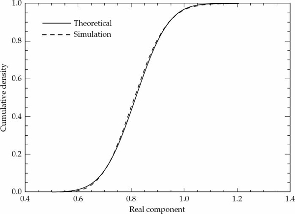
FIGURE 7.1 Cumulative densities for the real part of the sample ACS  for an AR(1) process with α = 0.99, τ = 20, and P = 10, 000. © Commonwealth of Australia 2011.
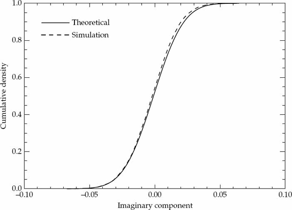
FIGURE 7.2 Cumulative densities for the imaginary part of the sample ACS for an AR(1) process with α = 0.99, τ = 20, and P = 10, 000. © Commonwealth of Australia 2011.
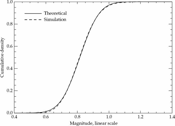
FIGURE 7.3 Cumulative densities for the magnitude of the sample ACS for an AR(1) process with α = 0.99, τ = 20, and P = 10, 000. © Commonwealth of Australia 2011.
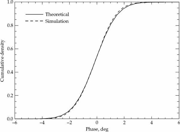
FIGURE 7.4 Cumulative densities for the phase of the sample ACS for an AR(1) process with α = 0.99, τ = 20, and P = 10, 000. © Commonwealth of Australia 2011.
7.3.3 Spatial Homogeneity Assumption
The Gaussian model for the temporal ACS of a skywave signal mode was experimentally confirmed by Watterson et al. (1970), but it was not possible for the authors of that work to determine whether the parameters of such a model could be assumed constant over all receivers in a very wide aperture array. In this experiment, the temporal ACS of each resolved propagation mode was computed separately in N = 30 receivers using 47 CPI of data collected over a period of about 4 minutes. The total number of samples available for estimating the temporal ACS in each receiver was 47 × 256 = 12,032. A set of Q = 30 uniformly spaced sample lags were calculated by averaging a sum of lagged products. The ACS starts at zero lag with consecutive lags equally spaced at multiples of 6 PRI (0.1 seconds) apart.
Using the ACS estimates computed separately in each of N = 30 receivers, the Gaussian model parameters were estimated for each resolved propagation mode using the method described in Section 7.3. The estimated temporal ACS parameters are shown in Table 7.1. Under the spatial homogeneity assumption, the Gaussian temporal ACS model estimated for a particular mode is assumed to have the same form in all N = 30 receivers up to a scaling factor cn. The ACS scale estimates cn resulting for the different receivers n = 1, …, N are not shown in Table 7.1, but will be analyzed in the next section dealing with spatial statistics.
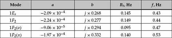
TABLE 7.1 Gaussian temporal ACS and Doppler spectrum model parameters estimated for the different propagation modes of the considered HF link.
Table 7.1 also lists the two parameters describing the Doppler power spectrum that corresponds to the estimated temporal ACS model. Specifically, the parameters f and Bt denote the mean Doppler shift (frequency displacement) and the Doppler bandwidth (frequency spread) of the Gaussian power spectrum, respectively. The mean Doppler shift is calculated as f = b/j2π Δt for a lag interval Δt = 0.1 seconds, since the model parameter b represents the change in phase per unit a lag interval. The mean Doppler shifts in Table 7.1 are practically the same as those estimated for the same modes using conventional processing in the previous chapter. The Doppler bandwidth is calculated as the inverse of the lag time for which the magnitude of the temporal auto-correlation function model falls by a factor of 1/e. For the Gaussian model, 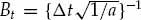 . The Doppler bandwidths in Table 7.1 are of the same order as those measured in Shepherd and Lomax (1967) and Watterson et al. (1970) on mid-latitude ionospheric paths.
Based on the hypothesized model for the statistically expected temporal ACS structure in each receiver, it is possible to derive confidence bounds for the experimentally measured sample ACS at each lag point using the theoretical results in Appendix A. At each lag point, these upper and lower bounds specify the interval expected to contain a certain percentage of sample ACS values when the random process is statistically described by the hypothesized model. If one or more lag components in the sample ACS are not contained within (say) the 90 percent confidence bounds, then there is strong reason to believe the hypothesized model is not suitable for describing the data. Conversely, when the entire sample ACS lies within the confidence bounds, there is no strong reason to reject the hypothesized model, which may then be accepted.
The solid line in Figure 7.5 shows the real component of the Gaussian ACS model for the 1Es mode based on the parameters estimated for this mode in Table 7.1. The dashed lines show the upper and lower deciles of the sample ACS distributions expected at each lag value under the assumption that this model is valid when 47 × 256 = 12, 032 data points are used to estimate the sample ACS. The experimental sample ACS measured in each receiver is first normalized by the estimated power scaling factor ecn for n = 1, 2, …, N. The resulting N = 30 sample ACS values computed using the experimental data at each temporal lag are then over-plotted using a + symbol in Figure 7.5. Figure 7.6, in the same format as Figure 7.5, shows the results for the imaginary component of the 1Es mode temporal ACS.
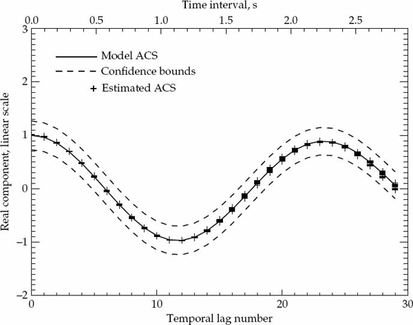
FIGURE 7.5 Temporal auto-correlation function for real component of 1Es mode. © Commonwealth of Australia 2011.
FIGURE 7.6 Temporal auto-correlation function for imaginary component of 1Es mode. © Commonwealth of Australia 2011.
The oscillatory behavior of the real and imaginary parts with respect to lag number is due to the mean Doppler shift. The higher the mean Doppler shift, the higher the frequency of these oscillations. The rate of decay of the amplitude envelope in both the real and imaginary parts is due to Doppler spread. The higher the Doppler spread, the faster the magnitude of the ACS falls with respect to lag number. Figures 7.7–7.12 show the results for the other modes in the same format. In all cases, the Gaussian temporal ACS model estimated for each mode in Table 7.1 agrees well with the experimentally observed sample ACS values measured in all N = 30 receivers.
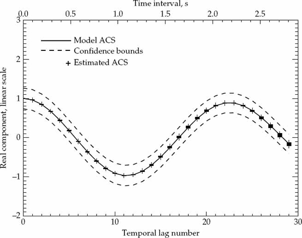
FIGURE 7.7 Temporal auto-correlation function for real component of 1F2 mode. © Commonwealth of Australia 2011.
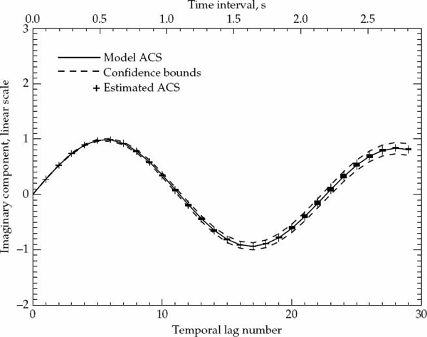
FIGURE 7.8 Temporal auto-correlation function for imaginary component of 1F2 mode. © Commonwealth of Australia 2011.
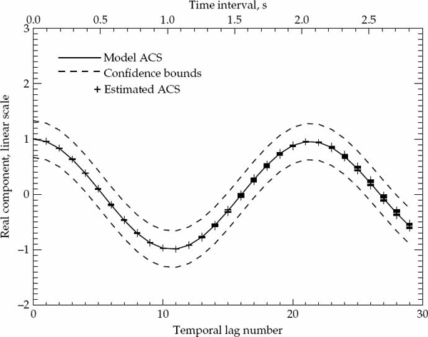
FIGURE 7.9 Temporal auto-correlation function for real component of 1F2(o) mode. © Commonwealth of Australia 2011.
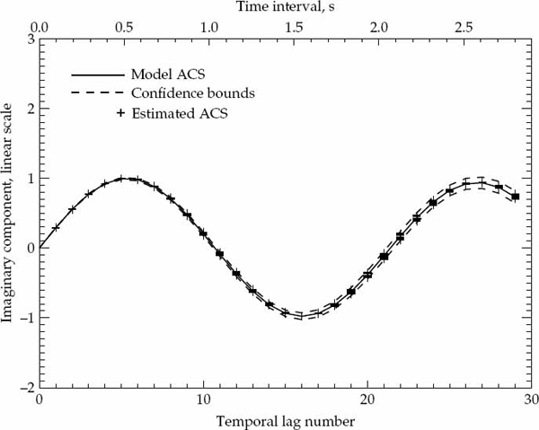
FIGURE 7.10 Temporal auto-correlation function for imaginary component of 1F2(o) mode. © Commonwealth of Australia 2011.
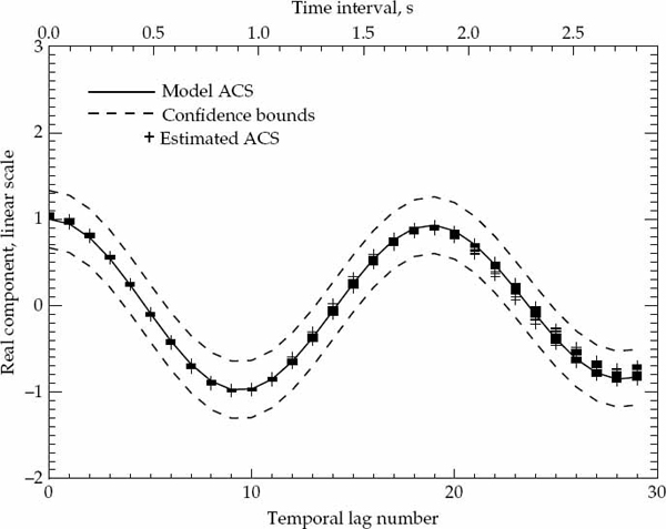
FIGURE 7.11 Temporal auto-correlation function for real component of 1F2(x) mode. © Commonwealth of Australia 2011.
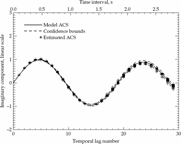
FIGURE 7.12 Temporal auto-correlation function for imaginary component of 1F2(x) mode. © Commonwealth of Australia 2011.
Based on these results, there is no strong reason to reject a Gaussian-shaped temporal ACS model for HF signal modes reflected by a relatively quiet mid-latitude ionosphere. This reconfirms the findings of Watterson et al. (1970) based on single-receiver data. In addition, the variability of the normalized temporal sample ACS across different receivers is almost always contained within the upper/lower decile confidence bounds. This observation, which could not be made on a single receiver by Watterson et al. (1970), leads to the conclusion that there is no strong reason to reject the assumption of spatial homogeneity for signal modes propagated by the analyzed mid-latitude HF channel. In other words, for a very wide aperture antenna array that spans a length of nearly 3 km, it has been demonstrated that the temporal ACS of these modes received at spatially separated points along the array can be described by a Gaussian model with the same mean Doppler shift and Doppler spread parameters. Apart from a possibly different power level or scaling of the ACS in different receivers, these results suggest that the temporal mode fading statistics can be assumed spatially homogeneous over very wide apertures for a relatively quiet mid-latitude HF channel.
7.4 Spatial and Space-Time Statistics
Mode wavefronts received due to signal reflection from a localized ionospheric region appear to have a mean structure that is planar with time-varying amplitude and phase modulations superimposed. The time-varying wavefront “crinkles” may be interpreted as a random spatial fading process that causes the angular spectrum of the received signal mode to spread around the mean direction-of-arrival (much like temporal fading causes the Doppler spectrum to spread about the mean Doppler shift). Assuming the spatial fading process is stationary over an observation interval of a few minutes, it is of interest to determine the validity of the spatial covariance matrix model in Eqn. (7.36). Such a model is consistent with the interpretation of the spatial fading process described above, and has been previously adopted to describe spatially spread signals in Paulraj and Kailath (1988) and Ringelstein, Gershman, and Bohme (1999).
(7.36)
In Eqn. (7.36), the symbol  denotes Shur-Hadamard or element-wise product,
  is the mean square value or power of the signal mode (assumed to be the same in all receivers), s(θ) is the steering vector of a ULA for cone angle θ, and B is an “angular spreading” matrix with its (i, j)th element equal to the magnitude of the spatial correlation coefficient between receivers i and j. This coefficient is defined as ρij in Eqn. (7.37), where
  for i, j = 0, …, N − 1 denotes the (i, j)th element of the statistically expected spatial covariance matrix Rx.

(7.37)
In this model, the mean plane wavefront is assumed to have a fixed direction-of-arrival that uniquely determines the phase of all spatial covariance matrix elements , just as the phase of the temporal ACS was solely determined by the mean Doppler shift. This is tantamount to defining the mean wavefront of a signal mode as the one that makes the real and imaginary components of the random modulation process statistically independent. In this case, the spatial modulations contribute only to the magnitude of the second-order statistics in Rx. For an arbitrarily defined mean wavefront represented by the N-dimensional vector s, the elements of the spatial covariance matrix based on such a model are given by Eqn. (7.38), where s[n] denotes the nth element of s.
(7.38)
When the mean wavefront is assumed to be a plane wave, the spatial covariance matrix Rx can be expressed in terms of the phase-only matrix s(θ)sH(θ) that determines the phase of all elements through the mean DOA parameter θ, and the real-valued matrix B that determines the magnitude of all elements through a parametric correlation coefficient model to be described shortly. Defining the phase  , the proposed model may be expressed in terms of the magnitude and phase of the spatial covariance matrix elements in Eqn. (7.39).
(7.39)
A model for the spatial correlation coefficients ρij in a very wide aperture antenna array has not been experimentally verified for resolved HF signal modes by formal hypothesis testing. Similarly, the plane wave model often assumed for the mean wavefront of an HF signal mode reflected from a localized ionospheric region has not been experimentally confirmed. The phase structure of the wavefront is important in applications where the signal is regarded as a desired signal to be received by the system. The correlation properties of the wavefront are of interest when the signal represents interference, as the correlation coefficients strongly influence the achievable cancelation ratio in adaptive spatial processing systems.
The synthesis of mean wavefront and correlation coefficient models yields a spatial covariance matrix model of the array data. For a stationary Gaussian distributed process, such a model completely defines the spatial statistics of a signal mode. This section develops a hypothesis testing framework that can be used to accept or reject formulated models for the mean wavefront and spatial correlation coefficients with a known level of confidence. The accuracy with which the experimentally measured two-dimensional space-time ACS of a propagation mode can be deduced from the product of its spatial-only and temporal-only ACS models is also quantified in this section (i.e., the assumption of space-time statistical separability).
7.4.1 Correlation Coefficients
The multiplicative amplitude and phase modulations are assumed to be described by a zero-mean complex Gaussian process that produces Rayleigh fading in the spatial dimension. This statistical description follows from the Gaussian scattering assumption validated by Watterson et al. (1970). Before proceeding to the validation stage, it is first necessary to describe a model for the correlation coefficients ρij in the matrix B. As for the temporal ACS, the Gaussian and decaying exponential amplitude envelope models are considered for the correlation coefficients.

(7.40)
In accordance with the assumption of a stationary process, such models assume that the second-order statistics of the spatial fading process depend only on the spacing between receivers d = |i − j| and not on their location (i, j) in the array. In practice, the real-valued model parameters a < 0 or b < 0 in Eqn. (7.40) that pertain to a particular propagation mode are not known a priori. These parameters may be estimated from the unbiased spatial sample covariance matrix (SCM)  calculated using real data in Eqn. (7.41).

(7.41)
For multivariate Gaussian snapshots xk(t), the spatial SCM represents the maximum likelihood estimate of Rx. Using the invariance property of the maximum likelihood (ML) estimator Kay (1987), it follows that the ML estimate of the magnitude of the correlation coefficient is given by  . As Rx is assumed to be a Toeplitz matrix, further averaging of the estimates may be performed over different receiver pairs spaced apart by an equal distance d = |i − j|. This yields the correlation coefficient function
  (d) in Eqn. (7.42), which is equivalent to the spatial ACS envelope normalized such that (0) = 1.

(7.42)
The values of a or b that provide the best least-squares fit between the real-data measurements 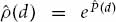 and the correlation coefficient model ρij = eP(d) in Eqn. (7.40) can be computed using the same parameter estimation method described for the temporal ACS in Eqn. (7.43). It is then a matter of assessing the significance of the departure between the assumed model and the sample estimates so that a decision can be made to accept or reject the hypothesized model with a known confidence level.

(7.43)
For a multivariate complex Gaussian distributed process, the sampling properties of the maximum likelihood estimate of the magnitude squared coherence 2 were found by Goodman (1963). If n statistically independent samples are used to estimate the magnitude squared coherence ρ2 between a pair of receivers, it can be shown that the distribution of the sample estimate 2 is given by Eqn. (7.44), where ρ2 is the statistically expected value.
(7.44)
The term F (x, y; w; z) is the classical hypergeometric function defined in Eqn. (7.45), where we have also defined (x)k = x(x + 1) … (x + k − 1). This series is guaranteed to converge if the argument of the function z has a modulus less than unity. In this case, we have that z = ρ22 < 1, so the function always converges. The density function p(2) was used in Carter (1971) for frequency domain coherence estimation. The same distribution may be used to derive confidence intervals that may be used to accept or reject the parametric model assumed for the spatial correlation coefficients.

(7.45)
As consecutive array snapshots are not statistically independent due to the significant temporal correlation, it is necessary to determine the equivalent number of statistically independent observations n to be used in Eqn. (7.44). For a large number of samples P, Priestly (1981) describes a method to determine the equivalent number of statistically independent samples for a correlated Gaussian random process. The first step is to compute the variance of the sample variance. For a complex random process, this is given by  in Eqn. (7.46), where r(k) is the expected correlation between data points spaced k samples apart and
  is the sample variance of the random process, as described in Thierren (1992).

(7.46)
Using Eqn. (7.46), the variance of the sample variance is r2(0)/P for P statistically independent samples as P → ∞. Hence, the effective number of independent observations for a correlated process is given by 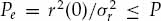 . The calculated value of Pe to the nearest integer may then be substituted for the number of independent samples n in Eqn. (7.44) to derive appropriate confidence intervals. If the estimates ij fall within the specified bounds for all receiver pairs (i, j), then the model for the spatial correlation coefficients is accepted, otherwise it is rejected.
The sample spatial covariance matrix used to compute the various correlation coefficients was estimated from N = 30 receivers using Eqn. (7.41), where P = 12,032 array snapshots (recorded in 47 dwells). For a separation of d receiver spacings, equivalent to d × 84.0 m in this experiment, there are N − d correlation coefficients that can be formed using P = 12,032 array snapshots. These N − d correlation coefficients were further averaged according to Eqn. (7.42) in order to form the envelope (d) used for model parameter estimation. It is postulated that an exponentially decaying function of receiver separation describes the behavior of the statistically expected spatial correlation coefficients. As the array snapshots used to form the sample spatial covariance matrix are correlated and therefore not statistically independent, an effective number of independent samples was also calculated using the procedure described in the previous paragraph.
Once the model parameter b is estimated from the SCM, and the confidence bounds are specified for the sample correlation coefficients based on an effective number of statistically independent samples, it is of interest to analyze the behavior of the estimated mode spatial correlation coefficients as a function of both receiver spacing and absolute position in the array. For a spatially stationary process, the correlation coefficient between two receiver outputs only depends on receiver separation and not the absolute receiver positions in the array. Hence, along with the mean wavefront analysis in the next section, this analysis will indicate the validity of both the spatial stationarity assumption as well as the exponentially decaying model proposed for the spatial ACS envelope.
Figures 7.13–7.16 show the hypothesized models for the propagation modes as solid lines and the associated confidence bounds (upper and lower deciles) as dashed lines. The actual estimates of the spatial correlation coefficients calculated from the experimental data have been overplotted using + symbols in each figure. There are more points marked with a + at smaller receiver separations because there are more pairs of receivers with such separations in the array. Clearly, only one estimate is available for the maximum spatial separation that occurs between the first and last receivers of the array.
FIGURE 7.13 Spatial correlation coefficients for 1Es mode. © Commonwealth of Australia 2011.
FIGURE 7.14 Spatial correlation coefficients for 1F2 mode. © Commonwealth of Australia 2011.
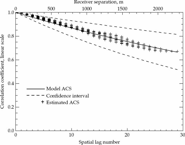
FIGURE 7.15 Spatial correlation coefficients for 1F2(o) mode. © Commonwealth of Australia 2011.
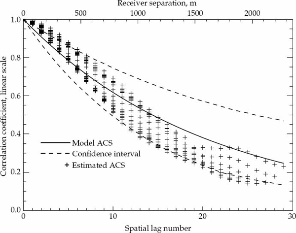
FIGURE 7.16 Spatial correlation coefficients for 1F2(x) mode. © Commonwealth of Australia 2011.
It is evident from Figure 7.13 that correlation coefficients estimated for the 1Es mode are not well described by the spatially stationary exponentially decaying model. This is not surprising because it was shown in the preceding chapter that this mode is likely to be composed of two sporadic-E reflections coming from distinct clouds of ionization that are unresolved in range but have significantly different angles-of-arrival. The superposition of two different spatial frequencies is expected to produce regularly spaced nulls (beating) in the spatial ACS. The first (imperfect) null is evident at a receiver separation of approximately 1150 m, while it appears that the correlation coefficient is falling toward a second null slightly past 2500 m. In contrast to the 1Es mode, the remaining signal modes are in very good agreement with the postulated statistical model. The great majority of the measurements lie inside the confidence bounds for these three other modes. Hence, for well-resolved signal modes reflected from a localized region in the ionosphere, there is no strong reason to reject the spatially stationary exponentially decaying model for the correlation coefficient over a relatively quiet mid-latitude path.
7.4.2 Mean Plane Wavefront
The plane wave s(θ) is the hypothesized model for the mean wavefront of a single propagation mode. In the presence of array manifold errors, the mean wavefront received by the system may not be planar. Even in the absence of such errors, it is conceivable that ionospheric phenomena may contribute to departures between the mean wavefront and the plane wavefront. To verify the mean plane wavefront hypothesis, it is first necessary to estimate the cone angle-of-arrival θ and amplitude A of the plane wave that best fits the mean wavefront  (extracted from the sample spatial covariance matrix) according to the least squares criterion in Eqn. (7.47).
(7.47)
From Eqn. (7.38), it follows that the magnitude of the mean wavefront |s[n]| at element n can be estimated as |[n]| in Eqn. (7.48), since ρnn = 1 by definition and the power scaling term  is taken into account by the amplitude parameter A in Eqn. (7.47). The phases
  for n = 1, 2, …, N can be found by solving a set of linear equations satisfying the phase difference relationship in Eqn. (7.48) using the elements (i, j) in the upper or lower triangle of the spatial sample covariance matrix. When all such elements are used, the equations become overdetermined for N > 3, and a least squares technique may be employed to estimate the phase structure of the mean wavefront.
(7.48)
Once the mean wavefront has been extracted from the sample spatial covariance matrix, the plane wave parameters of best fit may be estimated by performing a one-dimensional search for the minimizing cone angle-of-arrival  and amplitude Â. To assess the significance of the differences between the sample variances
  over the N receivers and the value Â2 expected for the assumed model, the distribution derived in Appendix A may be used to calculate confidence intervals for testing this feature of the model. For the mean plane wavefront model to be accepted, all of the sample variances are required to lie within the upper and lower deciles of the distribution. The reception channels are assumed to be well matched, and no allowances are made for potential differences between the gains of different reception channels.
Figures 7.17–7.20 show the mean power Â2 of best fit (solid line), confidence bounds (dashed lines), and the actual power estimated in the different receivers as “+” symbols for each propagation mode. The 1Es and 1F2(x) reflections have a significant number of measurements that lie outside the confidence bounds. This suggests the plane wavefront model is not representative of the mean wavefront for these propagation modes. In the case of the 1Es mode, this is understandable due to the two unresolved reflections that are present, but for the 1F2(x) mode, this result is somewhat unexpected and indicates that the spatial structure of the ionosphere that propagated this single magneto-ionic component was relatively more disturbed than the regions which propagated the 1F2 and 1F2(o) modes in the analyzed data. This is supported by the fact that the correlation coefficient measurements for the 1F2(x) mode in Figure 7.16 are comparatively more spread than those of the 1F2 and 1F2(o) modes. The 1F2 and 1F2(o) modes satisfy the constant power condition of the mean plane wavefront model.
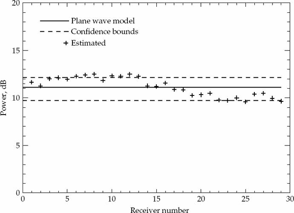
FIGURE 7.17 Power across aperture for 1Es mode. © Commonwealth of Australia 2011.
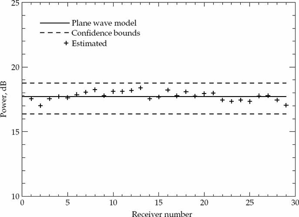
FIGURE 7.18 Power across aperture for 1F2 mode. © Commonwealth of Australia 2011.
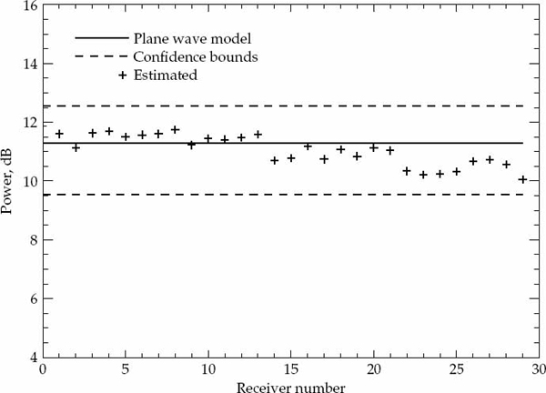
FIGURE 7.19 Power across aperture for 1F2(o) mode. © Commonwealth of Australia 2011.
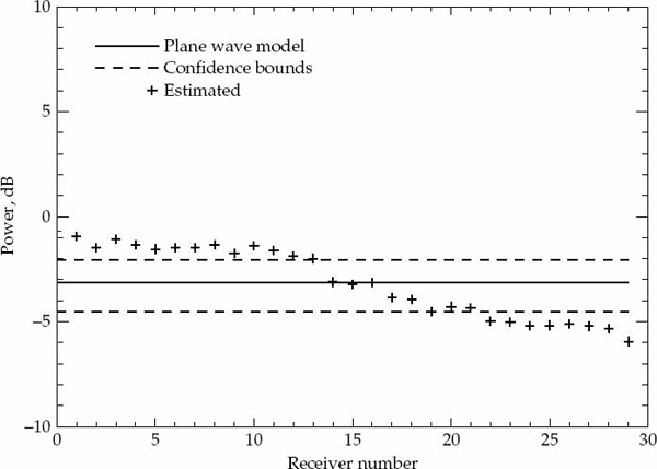
FIGURE 7.20 Power across aperture for 1F2(x) mode. © Commonwealth of Australia 2011.
To fully validate the proposed spatial covariance matrix model, it is also necessary to investigate the linearity of the phase across the aperture. The distribution for the phase of the temporal ACS derived in Appendix A may also be used for the phase of the spatial ACS. The latter is expected to be a linear function of receiver number with a slope that depends on the cone angle-of-arrival of best fit . Note that the distribution of the phase of a sample spatial lag about its expected value is identical to that of a sample temporal lag when the magnitudes of the expected correlations in the spatial and temporal domains are the same and the same number of samples are used to form them. Based on this equivalence, confidence intervals for the phase of the sample spatial lags may be derived using the formulas in Appendix A.
The expected linear phase progression of the spatial ACS is calculated for each mode using the corresponding estimate of the cone angle-of-arrival of best fit . Since the spatial sample covariance matrix is Hermitian, all of the information is contained in the elements of either the upper or lower triangle of the matrix (including the main diagonal). It is therefore required to check whether the phase progression of the elements in each column of either the upper or lower triangle of the spatial SCM falls entirely within the established confidence bounds. For the plane wavefront model to be accepted, all of the sample spatial lag phases are required to lie within the upper and lower decile confidence bounds relative to the linear phase front of best fit.
Figures 7.21–7.24 show the mean linear phase-front (solid line), the upper and lower confidence bounds (dashed lines), and the estimated phases corresponding to different spatial lags and reference receivers (“+” symbols) for each of the propagation modes. More than one symbol appears for all but the largest lag number in Figures 7.21–7.24 because each receiver in the array may be designated as the spatial phase reference. In all figures, the right vertical axis shows the cone angle-of-arrival, which depends on the slope of the linear phase-front. The cone angle of best fit for a particular propagation mode is indicated by the intersection of a straight line from the origin with the right vertical axis.
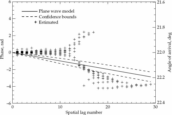
FIGURE 7.21 Phase measurements across the aperture for 1Es mode with different receivers in the array used as the spatial reference. © Commonwealth of Australia 2011.
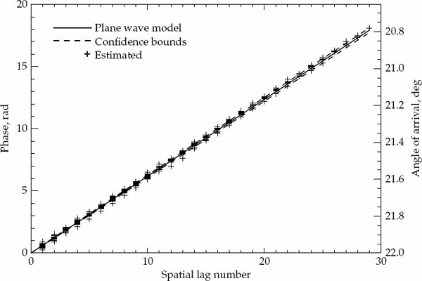
FIGURE 7.22 Phase measurements across the aperture for 1F2 mode with different receivers in the array used as the spatial reference. © Commonwealth of Australia 2011.
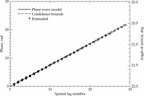
FIGURE 7.23 Phase measurements across the aperture for 1F2(o) mode with different receivers in the array used as the spatial reference. © Commonwealth of Australia 2011.
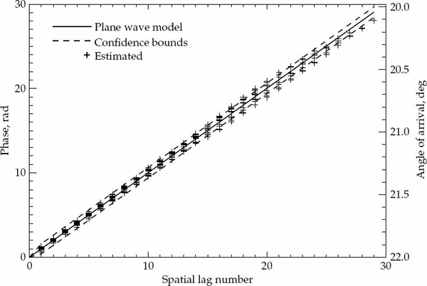
FIGURE 7.24 Phase measurements across the aperture for 1F2(x) mode with different receivers in the array used as the spatial reference. © Commonwealth of Australia 2011.
As for the power measurements, it should be kept in mind that phase measurements are also affected by instrumental errors such as phase mismatches between the responses of different reception channels. Despite the potential existence of these mismatches, it was assumed that the receivers were identical and no allowance was made to account for the potential influence of calibration errors by widening the confidence bounds. If the model is valid and such errors are present, more than the expected percentage of measurements are expected to lie outside the confidence bounds calculated under the assumption of no errors. Hence, the presence of gain and phase mismatches between the responses of the reception channels will tend to favor the rejection of plane wavefront model.
It is clear from Figure 7.21 that the 1Es mode is far from having a planar phase-front. This is expected due to there being two reflections with significantly different cone angles-of-arrival. Figures 7.22 and 7.23 indicate that the mean wavefront of the 1F2 and 1F2(o) modes have much more linear phase-fronts. The majority of the phase measurements made on these two modes fall within the confidence bounds. As the constant power assumption has already been validated for the 1F2 and 1F2(o) modes, it follows that there is no strong reason to reject the mean plane wavefront model for these two modes. A higher spread of the phase estimates is observed for the 1F2(x) mode in Figure 7.24, but the large majority of the measurements lie within the confidence bounds. This aspect of the plane wave model appears to be valid for the 1F2(x) mode despite the fact that the power of this mode varied beyond the confidence bounds across the aperture.
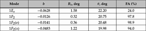
TABLE 7.2 Decaying exponential spatial ACS parameters estimated for the different propagation modes. The fitting accuracy achieved by the separable space-time ACS model is also listed.
The spatial ACS model parameters resulting for all modes are listed in Table 7.2. The parameter b in Table 7.2 is the coefficient of the estimated exponentially decaying function in Eqn. (7.40) for a receiver spacing of 84 m. The cone angle of best fit estimated according to Eqn. (7.47) is listed as θ in this table. The spatial bandwidth Bs of the signal mode is calculated by first determining the distance at which the magnitude of the spatial ACS falls by a factor of 1/e. The inverse of this distance is then computed to yield a spatial frequency in units of m−1. This spatial frequency may be expressed in terms of a cone angle for the ULA at the operating wavelength. This cone angle, which is a onesided measurement of the width of the angular spectrum, is then doubled to provide a measure of spatial bandwidth or angular spread given by Bs = 2 × arcsin (bλ/Δd) degrees. Spatial bandwidths of around 1 degree at a frequency of 16.110 MHz agrees well with the previous experimental results described in the opening section of this chapter.
7.4.3 Space-Time Separability
It is of interest to determine whether the sample space-time ACS  (Δd, Δt) measured from experimental data can be represented with reasonable accuracy in terms of the previously validated temporal-only ACS rt(Δt) and spatial-only ACS rs(Δd) models. The expected second-order statistics of a stationary space-time random process are said to be separable when the space-time ACS r (Δd, Δt) can be expressed as a product of the temporal-only and spatial-only ACS, as in Eqn. (7.49).
(7.49)
Hypothesis tests maybe derived to accept or reject space-time separability of the model by using the results in Appendix A. A simpler method for measuring whether a separable model is accurate is to quantify the fitting accuracy between the separable model of the space-time ACS r(Δd, Δt) in Eqn. (7.49) and the sample space-time ACS (Δd, Δt) estimated directly from the experimental data. A separable model may be considered appropriate when the fitting accuracy defined in Eqn. (7.50) exceeds a relatively high value of say 95 percent. The fitting accuracy is computed by synthesizing a space-time ACS model according to Eqn. (7.49) using the previously estimated Gaussian temporal ACS and exponentially decaying spatial ACS models for each propagation mode. The fitting accuracies resulting for the different propagation modes over 900 space-time lag points (i.e., 30 spatial lags times 30 temporal lags) are also listed in Table 7.2.

(7.50)
As expected, the space-time ACS of the 1Es mode is not well represented by this separable model because the spatial ACS model was previously rejected. The 1F2 and 1F2(o) modes are very well represented by the separable space-time ACS model indicating that for these modes the sample space-time ACS can be deduced with high accuracy from a knowledge of the experimentally validated temporal-only and spatial-only ACS models. The 1F2(x) mode is quite well represented by the separable model but not as well as the other two F-region modes. This may be due to the relatively more disturbed characteristics of the 1F2(x) mode in the analyzed data set, which caused the mean plane wavefront model to be rejected for this single magneto-ionic component.
Figures 7.25–7.32 illustrate the match between the experimental sample space-time ACS and the parametric model of a separable space-time ACS in terms of the real and imaginary components for each of the different propagation modes. Although 900 space-time lags were used to compute the fitting accuracy, only 100 space-time lags (10 spatial lags by 10 temporal lags) are displayed in these figures for clarity. The 10 lags chosen in each domain correspond to every third lag such that the plotted components are given by  for i, j = 0, 1, …, 9. These data points have been stacked into a one-dimensional vector referenced by the space-time lag index
  = i × 10 + j. The ability of the parametric and separable space-time ACS model to almost exactly replicate the experimental sample space-time ACS over 900 lag points in Figures 7.27 and 7.28 indicates that the second-order statistics of single modes reflected by the mid-latitude ionosphere can be well represented in a statistical sense by the postulated stationary and separable space-time ACS model over time intervals of a few minutes.
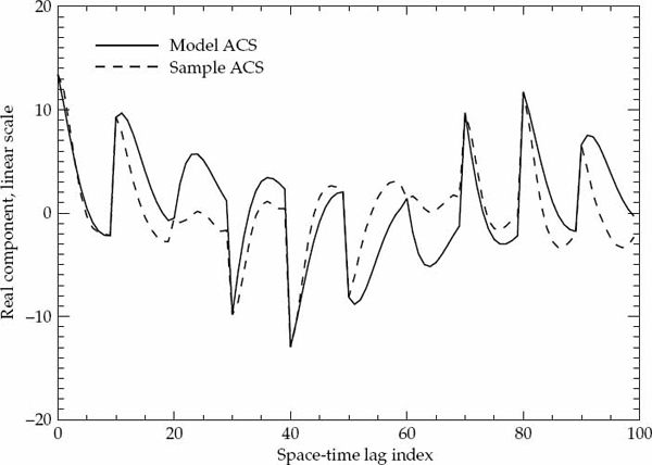
FIGURE 7.25 Real component of space-time ACS for 1Es mode. © Commonwealth of Australia 2011.
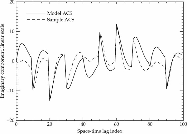
FIGURE 7.26 Imaginary component of space-time ACS for 1Es mode. © Commonwealth of Australia 2011.
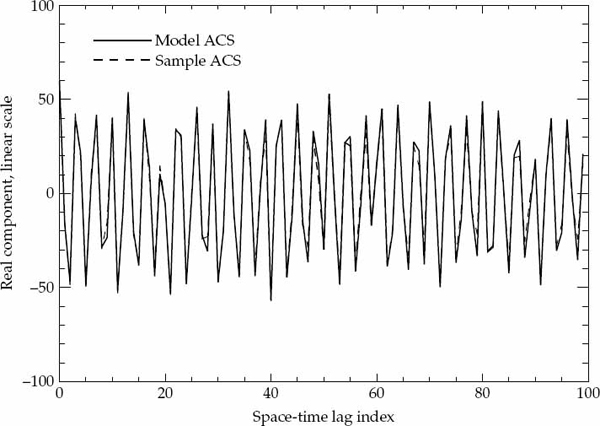
FIGURE 7.27 Real component of space-time ACS for 1F2 mode. © Commonwealth of Australia 2011.
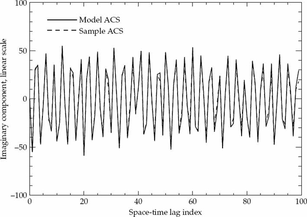
FIGURE 7.28 Imaginary component of space-time ACS for 1F2 mode. © Commonwealth of Australia 2011.
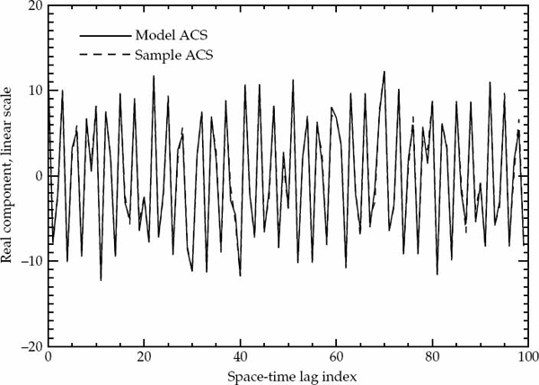
FIGURE 7.29 Real component of space-time ACS for 1F2(o) mode. © Commonwealth of Australia 2011.
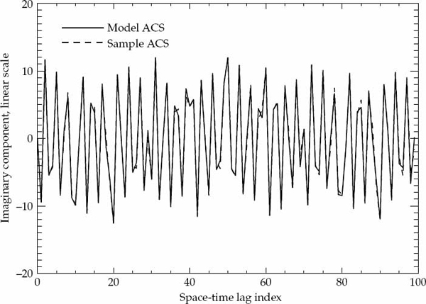
FIGURE 7.30 Imaginary component of space-time ACS for 1F2(o) mode. © Commonwealth of Australia 2011.
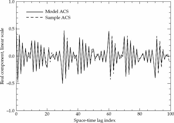
FIGURE 7.31 Real component of space-time ACS for 1F2(x) mode. © Commonwealth of Australia 2011.
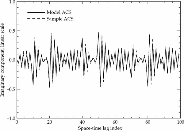
FIGURE 7.32 Imaginary component of space-time ACS for 1F2(x) mode. © Commonwealth of Australia 2011.
..................Content has been hidden....................
You can't read the all page of ebook, please click here login for view all page.