
Chapter 9
ELID Grinding with Lapping Kinematics
Ahmed Bakr Khoshaim*
Zonghua Xu†
Abstract
The demand for silicon carbide ceramics has increased significantly in the last decade due to its reliable properties. Sometimes, single side grinding is preferable over surface grinding, because it has the ability to produce flat surfaces. However, the manufacturing cost is still high because of the high tool wear and long machining time. Additionally, most of these grinding processes are followed by a lapping process. One of the ways to eliminate the lapping process is to use electrolysis in process dressing technique (ELID). Part of the solution also entails investigating the influence of different variables on the workpiece surface finish and material removal rate. This chapter presents the influence of the wheel #400 on the roughness and material removal rate. In order to do this based on the experimental results, a full factorial experiment was developed on three levels of each variable: the spindle and wheel speed, the applied load and the eccentricity. These four variables have been investigated and a model has been established for the roughness and the material removal rate individually.
Keywords
silicon carbide
SiC
fine grinding
material removal mechanism
electrolytic in process dressing
ELID
roughness modelling
MRR modelling
9.1. Introduction
Grinding is one of the most important abrasive processes. It is used to perform smooth and precise dimensions and surfaces. Usually, the material removal rate from the workpiece is low in grinding operations compared to that in milling or other cutting operations. However, it is considered effective for brittle materials. Finishing operations have a long history. Since the Stone Age, people were rubbing stones to create sharp edges. Also, the Egyptians had an amazing machining process for cutting large rocks, such as in the pyramids. Modern machining started in the nineteenth century [1].
In grinding, a grinding wheel with a number of abrasives adhered to it is used. The abrasives come in small pieces and in irregular shapes. In addition to the ability to resist chemical reaction caused by the lubricating fluid, the bond material should be strong enough to overcome the grinding forces and temperature. Many types of grinding wheels offer different configurations for different grinding operation conditions [2].
Abrasives and Wheel Types
Abrasives can be either conventional or superabrasives. Conventional wheels are cheaper than superabrasives wheels. On the other hand, superabrasives wheels are made with more expensive materials, and therefore, only a small part of the wheel is made by the superabrasives material where the rest can be made with metal. Conventional abrasives can be aluminum oxide (Al2O3) or silicon carbide (SiC). On the contrary, superabrasives can be either cubic boron nitride (CBN) or diamond. These last two are the hardest materials, which give them the ability to machine other hard materials. The hardness can be cited as Knoop hardness. For example, diamond hardness is 6500 kg/cm3, and CBN is 4500 kg/cm3. These levels are high compared to SiC and Al2O3 at 2500 and 1370–2260 kg/cm3, respectively [3]. The abrasives can be either small in size for better surface-finish roughness or large in size for higher material removal rate. The abrasives have the ability to fracture into pieces. This characteristic is called friability, which makes the abrasives self-sharpening. Very high friability and very low friability are undesirable. Very high friability makes the abrasives so soft that they are quite fragile. Low friability prevents the abrasives from breaking and sharpening themselves again, which will lead the abrasives to become dull. These abrasives have been made in the industry due to the amount of impurities in natural materials, which affects the reliability. The abrasives grain sizes are to be considered small compared to machining tools or inserts [4].
The six grinding wheel properties include the type of coating, the kind of dressing, the method and precision of balancing, the type of resin, the abrasives grit size, and the grain formula [5].
Grinding wheels come in a variety of types and sizes. They can be produced in many shapes, including straight, cylinder, straight cup, flaring cup, depressed center, and mounted. Both conventional and superabrasives wheels use different bond types. The two sheared bond types are vitrified and resinoid. A vitrified bond consists of ceramic bond mixed with the abrasives and shaped to the desired grinding wheel shape. Then, it is heated gradually to 1300 °C to allow the ceramic to create strong structure. Finally, it is cooled slowly and tested. Consequentially, in resinoid bonding, organic compounds are used and mixed with the abrasives, compressed, and shaped at a lower temperature of about 175 °C [3].
Metal-bonded grinding wheels have some advantages over the resin- and ceramic-bonded wheels, because metal-bonded wheels have high hardness and possess high heat conduction. Also, metal-bonded wheels have a high bondage capability, which gives the wheel a high holding ability for abrasives [6]. Sometimes, if the operation undergoes vibrations, but at the same time metal bond is needed for its electrical conductivity, a metal-resin-bonded grinding wheel can be used. Usually, this line of grinding wheels has a mixture of metal and resin bonds with a ratio of metal to resin at 7:3 [7]. Other types of bonds, including silicate, rubber, elastic, epoxy, and oxychloride, are also on the market and are manufactured by select manufacturers.
Grinding wheels typically have a standard coding, or marking system, for wheels to show their properties. For instance, we may find this code on a grinding wheel: 30A 46 H 6 V XX. The A in the code indicates that the wheel is made out of aluminum oxide Al2O3 abrasives. Different letters indicate different abrasives (e.g., C = SiC, D = diamond, Z = zirconia). The number 46 is the grain size, which ranges typically from 4 (coarse) to 500 or more (fine). H is the grade, which ranges from A (soft) to Z (hard). The harder the wheel is, the better the finishing and stronger the abrasives holding, hence, the longer the wheel life. On the other hand, the softer the wheel, the faster the cutting ability. The number 6 is the structure or the number of spaces between the bond and the abrasives grains. The structure is on a scale of 1–15, where the grains are dense at 1 and open at 15, V is the bond type (vitrified) (e.g., M = metal, R = rubber, S = silicate, E = elastic, B = resinoid, O = oxychloride, P = epoxy), 30 and xx are the manufacturer’s symbol for abrasives and the manufacturer’s private marking bond type [8].
Material Removal Mechanism
Generally, the materials can be classified into either ductile or brittle materials. Ductile materials are more electrical and thermal-conductive. Also, they usually have a low melting point and high density compared to brittle materials. They also show some differences in the fracture toughness, where it is far higher in ductile compared to brittle material. However, brittle materials usually have higher Young’s modulus and lower surface energy [9]. Also, the crack growth rate is bigger in brittle materials. The crack growth rate usually depends on the crack length, which will be explained later [10]. Brittle materials are also different from ductile materials in their atomic bonding. Atomic bonding in ductile materials normally is metallic. On the other hand, atomic bonding in the brittle materials can be either covalent or ionic, or both. Covalent bond has a higher thermal conductivity and a lower thermal coefficient of expansion than the ionic bond. Brittle materials with both types of bonding have different properties, depending on the ratio of the ionic/covalent bond in the material. For example, Al2O3 has a ratio of 6:4 ionic/covalent bond, where it is about 1:9 in SiC. This difference makes SiC preferable for use in higher-temperature applications, because the elevation of the temperature affects ionic bonding strength significantly [9].
Brittle materials are more challenging to machine than ductile materials, not only due to high hardness, but also due to easy fracture. The fracture most likely occurs in brittle materials in two ways: Either at the edges of the bond of the grains, which is called an intergranular fracture, or through the grains themselves, which also known as a transgranular fracture. Unlike brittle materials, ductile materials fracture mainly through the grains. However, another fracture type is called the chevron pattern. This type happens when the crack is spread over different levels of the material in a circular shape away from the impact. This crack can easily show the crack starting point and can be recognized by bare eyes or by microscopes [11]. Cracks in grinding ceramics can be either pulverization or microcracks. A consequence of one or both types of fracture – intergranular or transgranular – cause the pulverization crack. However, microcracks can be also categorized into scattered and clustered. Highly brittle material usually is not affected by clustered microcracks [12].
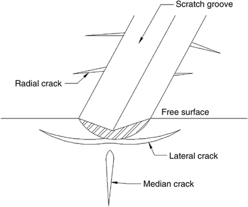
During the grinding of a brittle material, the material from the workpiece is mainly removed by two general principles. When a grain on the grinding wheel comes into contact with the workpiece, a chip from the workpiece is formed. This formation can be in either a ductile mode or brittle mode. Ductile mode, which is also known as a quasiplastic cutting mechanism, is preferred over the brittle mode. During the ductile mode, the chip formation result in grooves with no cracks, giving the grooves a smoother surface profile. On the other hand, brittle mode, which can be referred to as microbrittle mode, is not preferred. In this mode, the grooves created affect the surrounding area, forming surface fractures and cracks. These cracks can be one or more of the following types of cracks: lateral, radial, or median cracks. Some other cracks have also been reported, such as fork, branch, and chevron [13]. In a case of a brittle mode removal, a careful choice or modification of grinding parameters can turn this grinding process into the desirable ductile mode [10]. A stage in-between is called the brittle-ductile mode, semiductile mode, or partial-ductile mode [14]. In this mode, the material is removed at brittle mode and does not affect the material by forming advanced cracks underneath the material workpiece surface. Still, at this stage, the surface of the workpiece reaches the limits of high surface stresses. In order to reach this stage and not exceed it into brittle mode requires a careful choice of grinding parameters. A laser-assist can be used to preheat the surface of the workpiece before it enters the grinding process. This process helps reduce any brittle mode material removal and enhance the surface quality and roughness of the machined workpiece [10]. If the workpiece machining was in the brittle mode, this will produce a fractured surface that requires additional machining processes of lapping and polishing. Nonetheless, if the properties have been changed accordingly so that the machining process was in the semiductile mode, the surface of the workpiece will be partially fractured; thus, it will need direct polishing only. When we control the machining flawlessly so that the grinding is performed in the ductile mode, the finished workpiece material will undergo little or no polishing process [15].
It has been reported that the depth of cracks can be predicted. The experiment of the prediction involves grinding of a silicon wafer machined by a diamond grinding wheel. The depth of the crack is approximately half the grain size of the diamond grinding wheel. So it can be observed that smaller grain sizes have better surface finish quality [13].
Figure 9.1shows the most commonly identified cracks that can occur during the brittle-mode cutting. Radial and lateral cracks are not as bad as a median crack. They both can increase the material removal rate and can be monitored. The median crack is critical, because it is more likely to be responsible for the failure of machinery parts in the industry when they propagate. The problem is that this crack is hidden under the surface and can be difficult to locate.
In grinding, each grain works individually to scratch the surface of the workpiece. The continuation of fast small scratches on the surface results in a material removal from the workpiece. For better removal rate, the scratches from the grains should be close to each other. One of the many factors that the scratching process depends on is the length of the tip of the abrasive grain, as well as how deep the plastic deformation applied on the workpiece is. Load and tip radius are other factors that affect the scratching on the workpiece. Inappropriate choice of these factors leads to undesirable scratches, which in turn lead to entering the brittle mode with either lateral or radial cracks, or both [17]. Finishing a workpiece by ductile mode with no surface fractures gives a great smooth workpiece surface that does not need any additional processes such as lapping or polishing. In order to achieve that, the depth of cut should be small so that only nanoparticles are removed, depending on the workpiece material properties. The energy required for removing a certain volume from a workpiece while in ductile mode is [18]:
Ep=HVp
Where Vp is the volume and H is the hardness. However, the energy required for removing material in the brittle mode is [18]:
Ef=δAf
Where Af is the fractured area, and δ is the crack surface energy per unit area. The hardness and δ are typically the same for some materials. The estimated relationship of critical depth of cut for brittle materials with other parameters that cannot be exceeded to be in the free fracture ductile mode is [19]:
dc∝(EH)(KcH)2
 (9.3)
(9.3)
Where dc is the critical depth of cut, E is Young’s modulus, and Kc is the fracture toughness. By adding a constant to the formula so it can be more useful [10]:
dc=0.15(EH)(KcH)2
 (9.3a)
Therefore, the maximum grit depth of cut or chip thickness should be less than the critical depth of cut [20]:
hmax=2Ls(VwVc)√aeds
 (9.4)
(9.4)Where Ls is the distance between the adjacent grits, Vw is the work speed (rpm), Vc is the peripheral wheel speed (rpm), ae is the wheel depth of cut (μm), and ds is the diameter of the wheel (mm).
Though difficult to evaluate, the crack length can be calculated from equation (9.5) [9]:
lc=[0.034(cotψ)23{√EHKc}]23Fi23
 (9.5)
(9.5)Where ψ is the indenter angle, and Fi is the indenter load. Then the estimated critical force applied before a crack forms is [9]:
Fcritical=ϖK4cH3
 (9.6)
(9.6)Where ϖ is a constant that depends on the indenter geometry, which can lead to calculate the depth of the indenter as [21]:
h=(cotψ)13(E12H)Fi12
 (9.7)
(9.7)However, the maximum chip thickness on ELID grinding, which will be explained in detail later, is disturbed by the bond strength of the grinding wheel. Consequently, it can be written as [19]:
hmax=2kLs(VwVc)√aeds
 (9.8)
(9.8)
Where k is the ELID dressing constant that is proportional to the input power, voltage, and current duty ratio:
k∝Ip,V,Rc
With the help of these expressions, the holding and grinding forces for a single grit can be obtained as [19]:
fh=k1σsag
fg=k2Shmax
Where fh is the holding force, k1 a constant related to the wheel topography, σs is the yield strength of the layer, ag is the holding area of grit, fg is the grinding force, k2 is a constant related to the material properties, and S is the sharpness factor.
With knowing the approximate number of grits per unit area, we can evaluate the total holding force as [19]:
Fh=NfhAg
Where Fh is the total holding force, N is the number of grits per unit area, fh is the holding force per grit, and Ag is the grinding area (mm).
Furthermore, the total normal and tangential force can be anticipated from resolving the force per grit:
Fn=NαnfgAg
Ft=NβtfgAg
The normal force can be obtained also from its relationship with the actual depth of cut (ADOC) [22]. (9.14)
Fn=F0+Cada
Where F0 is the break-in force while ADOC is zero, Ca is a constant that depends on grinding conditions, and da is the ADOC, which can be expressed in terms of the number of grinding passes. For the ith pass, the ADOC is [20]:
da=d0{1−[kwkw+ks]i}
 (9.15)
Where d0 is the wheel ADOC, kw is the cutting stiffness, and ks is the machine stiffness. By substituting the equation in the normal force equation, the normal force can be realized after the ith pass as [22]:
Fn=F0+Caa0{1−[kwkw+ks]i}
 (9.16)
This equation shows that with time and increasing the number of passes, the normal forces should stabilize and become constant. The same is true with increasing the number of passes, [kw/(kw+ks)] becomes zero for kw and ks, not negative, which will make the final normal force when its becoming constant as:
Fn=F0+Cada
Grinding Mechanism
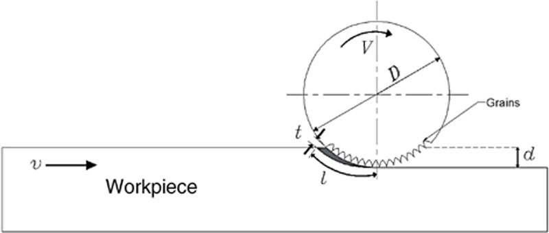
The abrasives are spread in the wheel randomly, and therefore have different rake angles, which is the angle of the face of the tool with the workpiece. These angles can be positive, zero, or negative. The rake angles usually are negative at about –60°. The wheel surface speed in conventional grinding is high compared to other operations, and it is typically from 20 to 45 m/s. However, in high-speed grinding, the speed can reach up to 150 m/s [23].
In grinding, each abrasive works as an individual cutter, as in single-point machining. However, they are different in many ways. For instance, the abrasive grains are arbitrarily separated, and each grain has an irregular shape. In addition to the highly negative rake angle and the high surface speed compared to the single-point machining during grinding, not all grains are active at all times [2].
Several parameters of the grinding operation can be observed by the following relationships [2]:
Undeformed chip length:
l=√Dd
Where D is the diameter of the wheel, and d is the depth of cut. Here, we are estimating this function, as d/D is small. In most operations, when d = 0.1D, the expression (9.19) will have an error of about 1%. Therefore, it is still a good approximation for the contact length [23].
Moreover, the undeformed depth of cut or chip thickness can be calculated as:
t=√(4vVtCnr√(dD))
 (9.19)
Where v is the speed of the workpiece, Vt is the rotational speed of the wheel, Cn is the number of cutting points per unit area, r is the chip width over the average undeformed chip thickness [2].
The general equation for the maximum undeformed chip thickness is [24]:
tmax=(E1E2)0.548√(4vVtCnr√(dD))
 (9.20)
Where E1 and E2 are the Young’s modulus of both the grinding wheel and the workpiece, respectively.
The parameter Cn can be estimated in the range of 0.1–10 /mm2, which is 102–103/in.2). It can also be estimated as [24]:
Cn=4fd2g(4π/3υf)23
 (9.21)
Where dg is the equivalent spherical diameter of diamond grains, f is the friction, and υf is the volume fraction.
The parameter r can also be estimated between 10 and 20. he is the chip equivalent and can be calculated as:
he=υfdVt
 (9.22)
Figure 9.2 illustrates these parameters for straight grinding wheel [2].
The tangential force of the grinding wheel is proportional to the grinding parameters, and it is smaller in comparison to the forces on other machining operations, due to the small active area of the grains. It is important to what energy is being dissipated during producing a grinding chip. This energy is called specific energy and is used to overcome the friction, plowing, and chip formation. This energy requirement can be found on tables as the required energy per unit volume of the material removed from the workpiece. Another two important parameters during grinding are the normal force and the cutting force. The normal force, which is also known as the thrust force (Fn), depends on the speed and the material removal rate [21]:
Fn=K.vQw
 (9.23)
The combination of the sharpness of the grains and the material being machined gives a constant known as the abradability constant (K). This force can be estimated to be greater than the cutting force by 30%. The cutting force, which is tangential to the wheel, can be calculated using this formula [2]:
Fc=P2πD2Nn
 (9.24)
Where P is the power and Nn is the speed. This function can be directed using the function:
P=Tω
Where T is the torque and is equal to:
T=FcD2
 (9.26)
And ω is the rotational speed:
ω=2πNn
The rotational speed is measured in radians per minute [2].
By assuming that the grains are spaced equally in the wheel, we can calculate the feed per grain, which is [21]:
s=v.TgL
Where TgL is the time of the grain first engages to the next engagement and can be calculated as [23]:
TgL=LVt
 (9.29)
Where L is the spacing between the cutting edges. The feed per grain can be rewritten as:
s=LvVt
 (9.30)
The calculated depth of cut is usually larger than the real depth of cut and that is due to the deflection of the wheel, workpiece, and the machine when the contact occurs. Therefore, we can calculate the depth of cut from the equation for the material removal rate (MRR). The material removal rate equation is [3]:
Qw=d.bw.v
Where bw is the width. The depth of cut can be written as:
d=Qwbwv
 (9.32)
In cylindrical grinding, if the workpiece speed is vy and the wheel wear is negligible, the depth of cut can be expressed as:
d=vynw=πdwvyv
 (9.33)
Where nw is the rotational speed of the workpiece and dw is the diameter of the workpiece, and can lead to the expression of the material removal rate for cylindrical grinding [23]:
Qw=πbwvfdw
The number of passes can also be used to express the material removal rate as [22]:
Qw=bwvfd0{1−[kwkw+ks]i}
 (9.35)
Finally, it has been determined that the total material removed by abrasive wear is also related to the lateral cracks size under the scratch line. A mathematical equation that describes the relation has been derived by Evans and Marshall [25]:
Vl=δcF98n(E/H)45(H58√Kc)
 (9.36)
Where Vl is the volume of material removed per unit scratch length, δc is a constant that depends on the material, Fn is the normal force or load, and E, H, and Kc are Young’s modulus, hardness, and fracture toughness, respectively. Jahanmir and Hockin showed the importance of including the grain size and microstructure properties of a brittle material in the removal model, which should also include the lateral cracks influence underneath the surface. The relationship between the lateral cracks and the material removal rate also depends on several conditions. For example, the crack can be strongly influenced if the grain boundary is weak. On the other hand, for polycrystalline ceramics, the relationship has been proven to be obscure. By studying the removal for repeated single-point scratches, the mechanism of material removal rate for ceramics can be observed [25].
Grinding forces can be expressed from the cutting model of grain edge as a combination of cutting components and friction components for both the normal and tangential force [26]:
Fn=cuttingn+frictionn=λkpam+knat
Ft=cuttingt+frictiont=kpam+μknat
Where kp, kn, λ, μ, am, and at can be defined, respectively, as the specific cutting force of the workpiece, the yield compression strength of the workpiece, the ratio of two components of force for the chip, the friction coefficient, cutting area of the grain edge, and the wear flatness area. The cutting area of the grain edge can be calculated as:
am=1nτυVt√tde
 (9.39)
A series of papers were published about fine grinding with mathematical modeling and experiments. One of the experiments has proved a predicted mathematical model of the grinding lines on a workpiece machined by a face-cup grinding wheel. It demonstrates a relationship between the ratio of the chuck, or spindle, and wheel speeds, and the distance between lines on the workpiece grounded. The relationship illustrates that increasing the ratio will increase the distance between lines. These lines are actually parallel curves, which are also affected by the ratio in their curvature [27].
Grinding Wheel: Close View
With a close view of the grinding wheel during operation, it was noticed that the grains interact with the surface of the workpiece mainly by cutting, plowing, and rubbing. Plowing and rubbing are undesired outcomes and will result in affecting the workpiece and increase the roughness. Plowing occurs when a grain slides over the surface without forming a chip, causing a surface change. Rubbing occurs when a loaded workpiece material is on the grinding wheel. Even though the grinding wheels contain a much harder material than the workpiece, wear begins immediately after starting the operation (Figure 9.3).
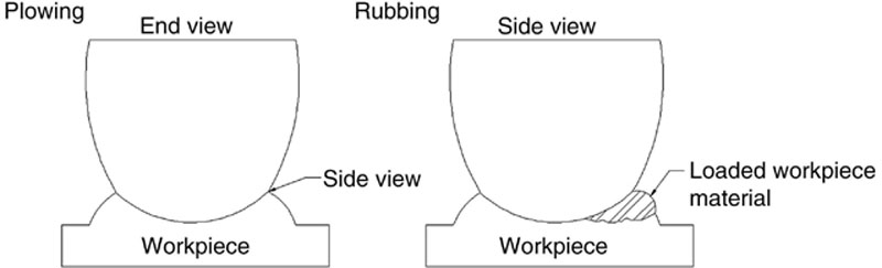
Figure 9.3 Grains intact with the workpiece
The best results from grinding occur when the rate of material removed from the workpiece is maximized, and the wear of the grinding wheel is reduced. In other words, increasing the grinding ratio of the wheel is accompanied by smooth surfaces and precise dimensions.
The wear that occurs to the grinding wheel can be classified in three mechanisms: attritious grain wear, grain fracture, and bond fracture. The attritious grain wear is similar to the flank wear in cutting tools. It occurs when the grains become dull, resulting in a wear-flat, where the grain slides over the workpiece without removing material and causes an undesired surface finish and high temperature. It is helpful to reduce the attritious wear by carefully choosing the material of the workpiece and the grinding wheel. Attritious wear becomes low if the workpiece and wheel materials are chemically inert. However, grain fracture can help the dull grains to be sharpened. The idea of grain fracturing is known as friability. Friability is useful, as long as it is in a moderate rate, so new grains are always and continuously presented. Bond fracture also plays an important character in the process of grinding. The bond needs to be chosen based on the material to be ground. For example, grinding a hard material needs a soft bond so it can reduce high temperature and residual stresses on the workpiece. Nevertheless, the bond should not be too soft or weak, which will make dislodging the grains too easy and result in an increase of the wheel wear rate. As a consequence, it will be hard to maintain dimensional accuracy in addition to an increase of the workpiece production cost. On the other hand, grinding a soft material needs a hard bond to increase the material removal rate. Nonetheless, the bond should not be too hard, which prevents the dull grains from being dislodged and replaced with new grains. As a result, the grinding process would not be sufficient.
The Grinding Ratio
Because wheel wear is something that cannot be eliminated, the reliability of this wheel can be estimated by calculating the grinding ratio (G-ratio), which is the ratio of the volume removed from the workpiece to the volume of the tool wear [28].
G=Vworkpiece material removedVtool wear
 (9.40)
The G-ratio can be low at 1 or high at 1000. Both are considered not good. For instance, the low grinding ratio indicates that the tool wear is too high, which can be expensive and economically inefficient. On the other hand, the high grinding ratio shows that the wheel is too hard for the workpiece material, which can cause an increase in the forces and lead to poor surface texture and vibration.
The value of the G-ratio depends on the grinding wheel, workpiece materials, and the fluid used. Using efficient fluid can increase the G-ratio significantly, which increases the wheel life and accordingly reduces the cost. Also, the G-ratio is not a parameter of the wheel, as the same wheel can have a high or low G-ratio. The G-ratio can be determined by the other parameters, such as speed of the wheel, depth of cut, and pressure, in addition to the workpiece material and fluid [2].
Grinding Types
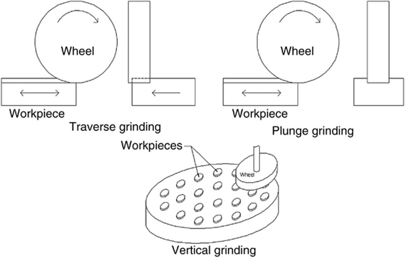
Among the many types of grinding, the most common are surface grinding, cylindrical grinding, internal grinding, and centerless grinding. Surface grinding is used to grind flat surfaces. The grinding wheel can be horizontal or parallel (vertical). Vertical wheel type uses a rotary table and can grind multiple workpieces at the same time. Horizontal wheels can travel across the direction of the workpiece, which is called traverse grinding, or travel along a groove in the workpiece in an operation is called plunge grinding. Figure 9.4 demonstrates the possibilities [2].
Horizontal grinding wheels can also be used with rotary tables, where it can grind multiple workpieces at once. Also, vertical wheels can work with reciprocating tables [29].
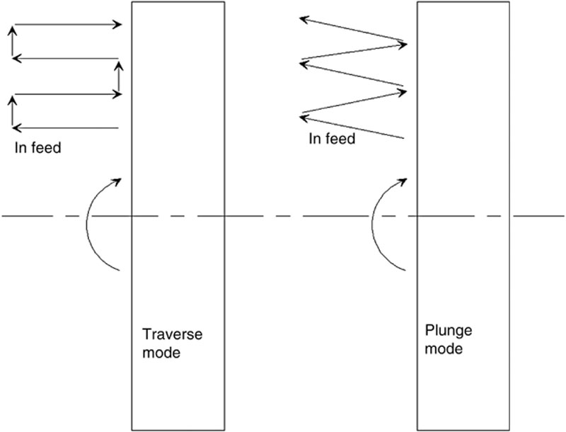
The feed rate on the grinding operation can be either traverse or plunge. In the traverse feed mode, the grinding wheel feed occurs in steps at the end of each grinding wheel pass. Conversely, in the plunge mode, the feed is considered continuous along the pass of the grinding wheel. Figure 9.5 demonstrates the differences.
Additionally, cylindrical grinding is for producing parts used in the auto industry, such as crankshafts, spindles, or pins. The workpiece is mounted from its axial ends. Both the workpiece and the grinding wheel rotate at different speeds from two different motors. Cylindrical grinding can be straight, by mounting the workpiece parallel to the grinding wheel. Cylindrical grinding can also be curved or steep, and can be performed to produce different shapes [2].
Moreover, the internal grinding has the same phenomenon as cylindrical grinding, except that it is for internal rotary parts. The internal grinding is a high-speed operation, because the grinding wheel rotates at a speed of 30,000 rpm or even more. Internal grinding can be one of three types: traverse grinding, plunge grinding, and profile grinding [2].
Finally, centerless grinding is typically the same as cylindrical grinding. However, as implied by its name, the workpiece is not mounted by its axial centers. This method is recommended for mass production and when small workpiece diameters are desired, such as engine valves, camshafts, pins, and any other similar component [23].
Other grinding types such as creep feed grinding are also performed. This type has the same kinematics of surface grinding, but also has a unique distinction as it removes a high amount of material from the workpiece. To help achieve the high removal rate, the workpiece speed should be low with a high-power grinding machine [3]. Usually the surface finish of the workpiece is lower than the other types of grinding, as finishing is not as important as the amount of material to be removed. In creep feed grinding, the depth of cut can be high; in some applications it can be up to 15 mm [2].
If a good surface finish is desirable for a workpiece that is machined by creep feed, an additional operation can be done to improve the surface finish. Usually a method called sparkout is used. The sparkout method uses no depth of cut. It is performed by barely touching the workpiece. This operation uses no coolant fluid, because the heat is desired to melt the external surface to smooth it. Sparkout operations become stable after three to four passes [28]. Some operations are used only for finishing operations. One of them is called belt grinding. Belt grinding can replace the traditional grinding in the finishing operations. It uses a belt with abrasives in a grit range of 16–1500 and can rotate at different speeds. To avoid vibrations and to achieve highly accurate dimensions, belt grinding machines necessitate being rigid [2].
Fine grinding is one of the grinding operations that uses the face of the grinding wheel, but also uses the kinematics of a lapping operation. Fine grinding has a constant pressure between the workpiece and the grinding wheel [7]. This project will focus solely on this operation and will be explained extensively later on. Despite the fact that conventional grinding undergoes high speeds and thus high temperatures, fine grinding, or grinding with lapping kinematics, is performed with low speeds and a much lower temperature, which will prevent any workpiece surface thermal damages. Fine grinding is performed on a lapping machine with bonded grinding wheels, providing advantages over the lapping process, including more speed, better accuracy, and cleaner parts.
Fine grinding is faster than the lapping operation, which will reduce the operating cost. This operation can be considered lapping with bonded abrasives, too [30]. Reducing the operating time not only reduces the power consumption, but also the labor operating time. Fine grinding with the correct choice of wheel and grinding parameters can give a precise dimensional accuracy and reduce the finishing operation time. In addition, fine grinding uses coolant fluid for cleaning and removing swarf to prevent loading. It does not use loose abrasives or slurry during the operation, which gives a cleaner overall environment. Moreover, fine grinding can be automated. Automation is becoming widespread to reduce the cost of labor and for more accurate results. Lapping will need additional cleaning operation, because these workpieces are not as clean as the ones from fine grinding [32]. Fine grinding can be either single side or double side. In this project, single side is used as shown in Figure 9.6.
9.2. Fundamentals of ELID
The ELID process can eliminate the use of lapping or polishing operations as a final stage. In addition, ELID grinding can provide better accuracy even though the grinding wheel wear is considered high when machining ceramics [6]. However, flatness is good in lapping compared to grinding operations, while some researchers claimed that ELID grinding with lapping kinematics, whether single or double side, can give similar flatness and reduced waviness in lapping operations. This approach can prevent the disadvantage of lapping when loose particles are dosed exceedingly in the operation, which is not economically appropriate, especially when using superhard abrasives [33].
Machining operations consist of inputs and outputs. The output is more important; we tend to change the inputs in order to gain certain outputs. Surface integrity is one of the most important outputs. Surface integrity output can have multiple measurements including the surface finish and freedom from cracks, chemical change, adverse (tensile) residual stress, and thermal damages such as burn, transformation, or overtempering. Surface finish is by far the most important of them all. Surface finish roughness has many values including Ra, Rv, Rt, and Rq. The most important measurements are Ra and Rt, where Ra is the average peak-to-valley distance, and Rt is the maximum roughness signal of the profile [34].
History
This process of dressing method is used for metal-bond wheels, and it is considered a new technology discovered in 1985 by Murata. The process has been extensively developed and enhanced since 1990 by Japanese researcher Hitoshi Ohmori [35]. This technology is useful when low roughness is needed or when machining hard materials using small grains to avoid cracks [23]. The idea of using electrical power for an in-process dressing came originally from a process called electrochemical grinding (ECG) [10]. Electrolytic in-process dressing (ELID) is a technology that enhances the grinding efficiency by increasing the removal rate and reducing the forces of the grinding process. This result is true when we continue the grinding operation for a period of time, because the material removal rate does not decrease significantly compared to that in conventional grinding. However, the reduction of the grinding forces occurs at the beginning of the process, but ELID can also provide constant forces as the process is being stabilized. The increase of the efficiency is essential machining ceramics because the cost of manufacturing them is relatively high with the low material removal rate, long dressing time, long machining time, and high tool wear [36]. Additionally, according to an experimental article entitled “High Efficiency ELID Grinding of Garnet Ferrite,” ELID grinding forces are lower than those in conventional grinding. The experiment has been conducted with the same parameters for both resin-bond diamond wheel and cast iron diamond wheel with ELID technique. The results show that ELID grinding with cast iron diamond wheel has about one-half the tangential and normal forces of the resin-bond diamond wheel [17]. ELID grinding also provides better surface topography than conventional grinding, which has been proven under the microscope experimentally [35].
A huge increase in the demand for ceramics in the industry can be attributed to their high temperature resistance, light weight, chemical stability, and their minimal lubrication. Ceramics can be also used in many applications including cutting tools, the auto industry, and aerospace industry. The problem is that with conventional grinding operations, the process cannot be continuous because the grinding process needs to be stopped for the wheel dressing. ELID technology has the ability to perform dressing for the wheel while it is in operation [36].
According to the article “Electrolytic In-Process Dressing (ELID) and Super-Precision Grinding for Ring Raceway of Ball Bearing,” ELID grinding has been investigated for the raceway of ball bearings. The results show that ELID grinding can replace or eliminate the use of the final finishing process of lapping or polishing. Elimination of this step is helpful because the final process of superfinishing with oilstone is complex and requires additional equipment [6]. In other research, ELID grinding has been compared with a non-ELID grinding for TiAIN. The results show that ELID grinding offers a slightly better average roughness (Ra), but a significant Ry, (Ry = Rt), improvement, whereas Ra and Ry are almost the same at ELID operation. However, the atomic force microscopy (AFM) 3D topography shows a huge difference between ELID and non-ELID grinding, where the workpieces with ELID were smoother with a greater surface finishing than non-ELID operation [37].
The ELID technique has been also applied to grinding X-ray mirrors. The experiment gave better roughness, but use of a pressurized method such as lap grinding was recommended [38]. ELID grinding with lapping kinematics produces no thermal damage or burn to either the grinding wheel or the workpiece due to the low speed of the operation [33].
The investigation on ELID technology also has been performed with acoustic emission. The acoustic emission technique helps in recognizing when the wheel is having any loading [39]. In other experiments, the acoustic emission was used to identify when the grinding wheel first touches the workpiece in face grinding [40]. One of the experimenters combined the ELID grinding with magnetorheological finishing process (MRF). The results show a better surface quality. Also, the outcomes show better efficiency: the MRF does not harm the surface as in conventional grinding, which will lead to a longer workpiece operational life [31].
In a paper by the Japanese researchers Itoh and Ohmori, an ELID lap grinding similar to the present project was performed with multiple wheels of varying mesh sizes including #1200, #4000, and #8000 and a coolant solution of 2% in water for silicon and tungsten carbide workpieces. The electrical characteristics were Eo 60 V, IP 30 A, and τ on/off 2 μs. The effect of ELID was obvious on two points. First, the improvement of the surface roughness and quality was excellent. And second, the removal rate was more stable and constant with time compared to a non-ELID operation. This paper also showed that using a complex material can reduce the resultant roughness in an insignificant manner [41].
Furthermore, Ohmori and Bandyopadhyay investigated the surface of a machined silicon nitride, and the results show a significant improvement of the surface after monitoring the workpieces with scanning electron microscopy (SEM) and AFM. One of the methods to ease the reading for these images is to coat the workpieces with Au-Pd. The images will show white spots as a sign of surface fragmentations and that the workpiece has been machined in brittle mode. If no spots are located, it is an indicator that the workpiece has been machined in ductile mode [36]. The results of that experiment show that grinding with ELID using #4000 mesh size or finer gives a continuous ductile mode machining in addition to the significant reduction of the bend strength [42].
We always tend to reduce the grinding forces. High grinding forces explain some difficulties in grinding and that the abrasive grains have a hard time cutting though the workpiece. According to the article “Study on the ELID Grinding Forces of Ceramics and Steels,” even though ceramics have higher strength than steels, grinding forces in steels may have higher values than ceramics due to the strength of the steel in the initial chip formation, in addition to the high friction forces of the steel ships. Therefore, with the same grinding conditions, grinding force values vary depending on the grinding depth of cut, the longitudinal feed speed, and the traverse feed speeds [43].
ELID grinding was also investigated for biomaterials. Biomaterials that need specific flatness and smoothness are usually manufactured by polishing. However, due to some disadvantages of the polishing process, such as intrusion of an abrasive on a work surface, ELID technology has been tested for biomaterials. Mizutani, Komotori, and Nagata proved that ELID grinding can produce the same surface finish as polishing for some materials. Nonetheless, the results in their current experiment showed a significant difference in the maximum roughness even though the average roughness has no significant effect. Also, ELID grinding provides the best surface corrosion resistance at the passive stage due to the thick oxide layer [44].
ELID Equipment Requirements
What is needed for the process is any ordinary grinding machine with an electrical conductive wheel, a metal-bonded wheel. The only difference is the additional requirement of a power source to generate the required DC electric charge, in addition to a high PH electrolytic coolant. The connection of the system starts with connecting the wheel with the positive pole of the DC current anode with a smooth brush. The negative pole cathode, which is fixed, will be connected to an electrode made out of stainless steel or copper. This electrode will cover about one-sixth of the active area of the grinding wheel with a width about 2 mm wider than the wheel. The gap between the wheel and the electrode is adjustable and is typically 0.1–0.3 mm. The advantage of ELID is that it will continuously maintain the abrasive grains freshness, which will give a constant low roughness. The idea is to replace the worn abrasives and oxide layer continuously by balancing the voltage, current, and the gap. The ELID technology shares the same idea with electrochemical grinding (ECG), but the difference is that the function of ECG is to take away the substances from the workpiece [23]. ELID grinding can be equipped with a computer numerically controlled (CNC) machine. It has already been tested for a five-axis high precision CNC machine for ELID grinding with acceptable results [45].
The Mechanism of ELID Grinding
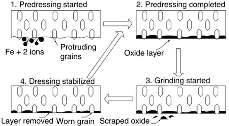
The mechanism is simple in explanation but complex in operation. When an electrical current passes through the electrode to the wheel with the present of a high PH coolant, this coolant will act as electrolyte. Electrolysis will occur and allow positive ions, also known as cations, to transfer from the grinding wheel to the electrode, mostly as Fe+2. Positive ions mean that they have missing electrons and are willing to receive these electrons when they come in contact with negative ions [60]. This contact will remove the metal bond of the wheel, which will protrude the abrasives. The continuation of the DC electrical pulse will form an oxide layer of Fe2O3 to coat the metal grinding wheel. It has a similar phenomenon to the electroplating process where the ions will transfer to the opposite side of the current flow. This layer of Fe2O3 is an electrical insulator, which will increase the electrical resistance of the wheel. With the accumulation of this layer, the current will decrease as the resistance increases. The whole system will reach equilibrium with an almost constant volt and current. The predressing process usually takes about 30–90 min. At this point, the grinding process starts. During the grinding process, the oxide layer will start to wear out along with some abrasives, which will reduce the electrical resistance. As a result, the current will increase, removing a new metal bond from the wheel and forming a new oxide layer, which will move the system to equilibrium. Figure 9.6 illustrates this mechanism [23].
Electrical and Chemical Aspects of ELID Grinding
The power of the electricity is divided into voltage and current. The power is constant during the operation while the current and voltage change alternatively. When the operation starts, the metal-bond grinding wheel has good electrical conductivity. The current is at its highest level, and the voltage is low between the grinding wheel and the electrode. After few minutes, the cast iron is removed by electrolysis and transforms iron ions mostly Fe2+. This transformation will hydroxide the ions to form Fe(OH)2 or Fe(OH)3. The reactants are based on the following chemical equations:
Fe→Fe+2+2e−Fe+2→Fe+3+e−H2O→H++OH−Fe+2+2OH−→Fe(OH)2Fe+3+3OH−→Fe(OH)3
 (9.41)
The reactants will oxidize and form (Fe2O3) on the wheel, which will reduce the electrical conductivity of the wheel. The current will be reduced from flowing by the increase of the resistance made by the accumulation of the oxide layer to an equilibrium point [23].
During the operation, the oxide layer starts to wear out along with the abrasive grains. This wear reduces the thickness of the oxide layer. The reduction will decrease the electrical resistance and increase the electrical conductivity. Thus, it allows the current to increase again and the electrolysis to make a new fresh layer. For ELID grinding, the described electrical behavior is nonlinear due to the formation of this insulating oxide layer. During the production of the second layer, more protrusion of active abrasive grains is used. Different types of grinding operation require different oxide layer thickness. For instance, if a fine surface is desired or for efficient ELID grinding, a thin layer is required so the grains can protrude out, which will help to increase the material removal rate. On the other hand, for finishing grinding operations that requires mirror finish, a thick layer is needed so the depth of cut can be limited. The variations of the oxide layer thicknesses can be controlled by the applied output current of the DC power source and with controlling the gap. For instance, increasing the current duty ratio gives thicker oxide layers. The current duty ratio is the on time to the total cycle time [35].
Rc=tonton+toff×100
 (9.42)
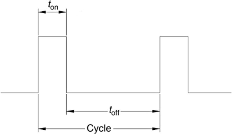
The oxide insulation layer has special characteristics, making the normal and tangential force increase and decrease periodically. When the normal force starts to decrease after it reaches the peak point, an immediate increase of the tangential force occurs because of the breakage of the oxide layer. The normal force starts to increase again with a new cycle of creating the oxide layer. This process repeats but the tendency of the normal and tangential forces is increased [46]. With this feature, fine and ultrafine finishing can be performed using the same wheel with the adjustment of the ELID power source and layer thickness [23]. In other words, increasing the current duty ratio gives a shorter time to reach a desired oxide layer thickness and a faster reduced working current. This process absolutely can be more economical. Conversely, neither overincreasing nor overdecreasing the current duty ratio will give better wheel surface conditions. The best wheel surface conditions can be observed using an intermediate range of the current duty ratio. At the same time, this intermediate range of current duty ratio offers better grinding performance with a smaller value of specific grinding energy and percentage of wear flat [47]. A careful choice of the current duty ratio is needed because of its relationship with the wheel wear. Increasing the current duty ratio will decrease the G-ratio, which means that the wheel will have higher wheel wear and less life. Forming an oxide layer while using a high current duty ratio will create a soft oxide layer that will be removed more easily while grinding and more abrasives will be pulled out. Therefore, using a low current duty ratio would form a harder oxide layer with higher bondage capability, and thus, longer wheel life [35].
ELID technology has been addressed in many publications showing that it has a positive resultant workpiece when grinding brittle materials such as glass or ceramics. With ELID, the need for polishing or lapping as a final step in many applications can be eliminated because the results satisfy the roughness requirement. ELID is better when it is used on small grit grinding wheels such as #4000 or finer. It has also been reported that the material removal rate has increased with ELID 32 times, and the grinding forces decreased with surface stresses about 150–400 MPa. In previous experiments, traverse feed mode gave better results in terms of surface roughness than plunge feed mode [28]. Farther more, in the article “Ultra-Precision Grinding of Hard Steels,” an experiment used conventional grinding and ELID grinding. The comparison showed that using ELID can overwhelm the pullout of the CBN grains. In addition, the surface finish for conventional and ELID grinding were almost the same at the feed rate of 5 mm/min. However, increasing the feed rate led to significantly increased roughness for the conventional grinding whereas the increase was negligible using ELID [48].
ELID Predressing Time
During the process of ELID grinding, the material is removed from the wheel by an electrochemical reaction. Because the small nonconductive diamond grains are embedded in a conductive metal bond, the removal of this metal by electrolysis most likely will be deviating. This reason makes it difficult to predict the predressing time of the ELID grinding. However, a prediction can be based on Hong and James’s model for electrochemical laws. This model finds the current density distribution around the diamond particles, which allows calculation of the material removal rate of the metal bond. The equations used for the calculations are [49]:
Faraday’s law for the metal removal:
dmadt=waζaFrJn
 (9.43)
Where dma/dt is the anode metal removal rate per unit area, wa is the atomic weight, ζa is the valence of the metal ions, Fr is Faraday’s constant, and Jn is the current density normal to the anode surface.
Ohm’s law for ion transport [49]:
J=−σe∇φ
Where J is the current density vector, σe is the conductivity of the electrolyte, and φ is electrical potential.
Steady-state current field law [49]:
∇J=0
These equations need some assumptions before they can be valid. For Faraday’s law, the assumption is that the rate is proportional to the current density. For Ohm’s law, the electrolyte has a uniform conductivity. The conductivities of both the anode and cathode are large so they are in an electric equilibrium, in addition to the assumption that the system is in steady state.
Researchers developed a formula for calculating the average current per unit metal area [49]:
Jn=1Sa ∫SaJndS=σ(VH)1−f[(πH2A)f(πH2A)f−ln(cos(π2)f)]
 (9.46)
This formula is for fixed gap and voltage. Now, by substituting the equation in Faraday’s law, we get [49]:
dmadt=WaζaFσ(VH)1−f[(πH2A)f(πH2A)f−ln(cos(π2)f)]
 (9.47)
By taking dt to the other side, an integrate per predressing time is calculated:
∫Tdmadtdt= ∫TWaζaFσ(VH)1−f[(πH2A)f(πH2A)f−ln(cos(π2)f)]dt
 (9.48)
This calculation then leads to the equation of the mass of the metallic layer removed:
ma=WaζaFσ(VH)1−f[(πH2A)f(πH2A)f−ln(cos(π2)f)]T
 (9.49)
Solving the equation for the time [49]:
Time=maWaζaFσ(VHgap)1−f[(πHgap2A)f(πHgap2A)f−ln(cos(π2)f)]
 (9.50)
Where A is the radius of diamond grains, Hgap is the gap, V is the voltage, and B is the distance in between two diamond grains over 2.
Equation (9.49) gives an understanding that increasing the voltage should reduce the predressing time. On the other hand, an increase in the gap should increase the predressing time. At the University of Toledo labs, some fixed values such as Wa = 55.845 g, and ζa = 2 have been established.
Although ELID grinding gives efficient results compared to conventional grinding, it is still a complicated process that needs to be adjusted for additional cycles of machining for optimum results, as incorrect parameters increase the tool wear and give an undesirable workpiece surface finish properties. These additional cycles can be reduced by the help of a feedback control system, which will increase the efficiency, and hence reduce the overall operating cost. Even though the elimination of the adjustment cycles is difficult, a feedback-based control system reduces the number of adjustments significantly. Basically, it has a computer-controlled system in which the operator can input the parameters such as the wheel parameters and the output workpiece finishing quality. The computer, with the help of the database, will start the system to the nearest optimum point where it can be adjusted to the optimum operation conditions after the operation started [50].
ELID Grinding Applications
ELID grinding has been used in experiments with many materials including ceramics, glass, and biomedical materials and with many grinding types. The advantage with ELID technology is that it can be applied to any machine. Therefore, many ELID types are presented, such as ELID surface grinding, ELID cylindrical grinding, ELID internal grinding, ELID centerless grinding, ELID CG curve-generator grinding, ELID aspheric grinding, ELID face grinding, ELID double-side grinding, and ELID lap grinding.
With surface grinding, it is essential to apply the ELID technology because it is the most common method of grinding. The ELID method can be applied to many surface grinding applications including the regular straight-type grinding wheel, with a rotary grinding system in a straight-type grinding wheel, and with in-feed grinding systems. Cylindrical grinding and internal grinding are the same idea except that cylindrical grinding is for external cylinders, where internal grinding is for internal cylinders. The ELID phenomena are the same for all grinding types. ELID has also spread to special cases as in the CG grinding. ELID aspheric grinding has been investigated for optical lenses and molds. ELID technique has even been extended to face grinding and double-side grinding. Finally, ELID lab grinding is similar to ELID double-side grinding except that it uses one wheel and a spindle. This operation is the main focus of this project and will be explained extensively later [51].
ELID Methods of Development
Many researchers have studied improvements of ELID technology use for special operation conditions. In previous investigations, ELID technology has proven that it can be applied with environmentally friendly operations, which implies a reduction of fluid supply using a mist spray. The method was tested and proven to work and achieve an oxide layer with a considerably environmentally friendly amount of fluid.
On the other hand, some applications including micro lens molds are using small grinding wheels. Other applications require the grinding wheel to be connected to the workpiece all over, all the time, as in honing operations. These cases are difficult to be dressed in process. A solution for these cases is suggested by performing the ELID dressing in intervals. In the first case, ELID predressing is performed prior to starting the grinding operation. After a while, the operation pauses and another ELID cycle is executed for another grinding interval because the grinding wheel is so small that it is challenging to attach a small electrode with the required gap to perform the ELID operation. In the second case where the wheel is connected continuously, attaching an electrode to the grinding surface area is impossible. This method of ELID is also known as ELID-II or ELID interval dressing.
Sometimes, the area where an electrode can be mounted on the grinding machine is limited. In this case, an electrodeless technique can be used with the workpiece as an electrode. This approach requires the workpiece to be made out of an electrical conductive material. By connecting the negative pole to the workpiece and with the presence of the coolant fluid, the ELID cycle completed. This method of electrodeless ELID is also known as ELID-III [51]. ELID-III has potential erosion caused by the sparks. A careful choice of electrical parameters such as small current duty ratio, low voltage, and low current can eliminate this problem [52].
Using an alternative current can improve ELID-III. A method called ELID-IIIA, which has no contact between the workpiece and the wheel, will improve the surface finish due to the elimination of any electrical discharge. The reason is that using an alternative current will create a thick oxide layer on the workpiece surface [53].
In some applications, a different method of ELID dressing without the use of an electrode is to have a conductive material on the tip of the grinding fluid nozzle. By connecting the positive and negative poles to the two conductive plates on the nozzle, ELID can be performed by an ion-shot method. In this method, the whole grinding wheel face is free and not covered by any electrode or connected to the positive pole [51].
In some cases, ED-trueing and ELID grinding can be performed at the same time. This process occurs by applying ED-trueing before the ELID grinding operation. Some researchers have reported that this idea gives the wheel a better and more accurate profile surface [52].
In a research paper, ELID technology also has been investigated on quartz blank, which is used in many telecommunication devices. ELID was used with wheel mesh sizes #325, #4000, and #8000.Wheel mesh size #325 was used by ELID I, and wheel mesh sizes #4000 and #8000 were used using ELID-II. The result from mesh size #325 was acceptable and near the desired condition. However, after further processing by ELID-II with mesh sizes #4000 and #8000 correspondingly, the results were positive with Rmax of about 0.060 μm [54].
Grinding with Lapping Kinematics in Certain Applications
This operation is also known as lap grinding, fine grinding, or flat honing. Fine grinding is usually used for superabrasives wheels while flat honing is more for conventional abrasives wheels. Grinding with lapping kinematics is helpful when the workpiece needs machined precision surfaces on a difficult-to-grind material such as hard ceramics [55]. It is recommended for use if a mirror finish is needed when it cannot be obtained with constant feed or by using wheels finer than JIS #10000 [23].
Lap grinding differs from regular grinding because it is considered a cool process with lower speed and no sparks. However, a flood of cooling fluid is necessary to control the temperature and to remove the swarf from the machined workpiece. If insufficient coolant is provided, wheel loading increases and surface finish will not be as expected, in addition to the possibility of thermal damage to the workpiece or the wheel. In the experiment, the proposed TRIM C270E, high-performance synthetic is initially used with a concentration of 5% with water. This coolant is provided from Master Chemical Corporation located in Perrysburg, Ohio. The TRIM C270E has a low ferrous corrosion inhibition with an electrical conductivity of 1.8 mS, refractometer factor of 3.3, and a pH of 9.0–9.3 (typically pH of 8.7–9.2) [56].
This process is often useful in parallelism and its use of two parallel grinding wheels. Nevertheless, this experiment contains one grinding wheel only. Usually, the stresses on the machined surface were easily relieved, and mirror surface finish can be achieved. The wheels of grinding with lapping kinematics are flat wheels made out of aluminum oxide (Al2O3) or silicon carbide (SiC). Aluminum oxide is cheaper but silicon carbide is better. Nonetheless, in some cases where the material to be machined is quite hard, such as in this experiment, a harder wheel is necessary, like cubic boron nitride (CBN) or diamond. These wheels become more expensive if the friability is higher, which will give new sharp grains faster. Friability is the ability of the grains to break down and expose new sharp edges, which will increase the material removal rate with more accurate tolerances [57].
Lap grinding also differs from conventional grinding because it has a constant pressure throughout the operation. The pressure of the wheel depends on the type of material machined. Harder workpieces require more pressure than softer ones. Lower than the recommended pressure is always better than going over the recommended pressure; it is only going to consume more time, whereas in overpressure cases, more heat can be generated, causing more damage to the wheel by pulling off grains, and indeed bad surface finish production [57].
General Principles of Grinding with Lapping Kinematics
Even though different from the present project, double-side lap grinding usually takes place with two wheels where the workpiece is guided between them with a workpiece holder, and it is free to align itself. In addition, the flatness of the wheels is maintained precisely, and the pressure applied to the workpiece by the wheel causes the cutting action. A flood of coolant is always necessary to lubricate, cool, and clean the workpiece. Conversely, the present project uses the same principles except that the cutting medium is only one flat grinding wheel, and the workpiece is held stationary in the workpiece holder (see Figure 9.8). Lap grinding is useful to correct many properties including flatness, parallelism, surface roughness, and dimensional accuracy [57].
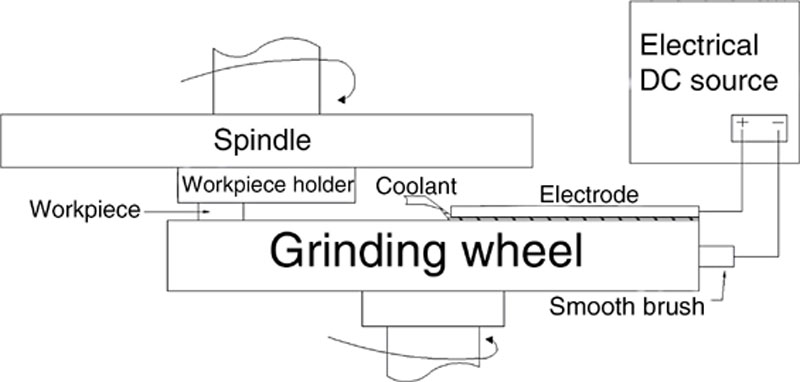
Figure 9.8 Single side ELID grinding
Lap Grinding Modes
Several modes of lap grinding are used in the industry such as batch-mode processing. Batch-mode processing is useful for mass production where the machine is loaded with the maximum number of workpieces. They are all machined at the same time, which ensures equal thickness machining from each workpiece, and almost the identical roughness and material removal rate. Another mode is called through-feed mode. In this mode, the workpiece passes through the wheels only once. This method is helpful for small workpieces. If more material needs to be removed, multiple passes can be applied [57].
In general, dressing takes place when a hard ceramic or diamond dresser abrades with the grinding wheel. Therefore, because the wheels used in this project are made of diamond and with small grid sizes, traditional methods cannot be used for dressing. Other methods can be used such as abrasive-jet, slurry dressing, and high-pressure water jet. Some of the new methods for dressing are performed during the grinding operation, such as electrodischarge machining or laser dressing, in addition to ELID [58] (Figure 9.9).
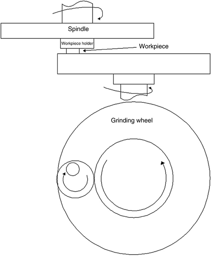
Figure 9.9 Single-side grinding with lapping kinematics
Cutting Fluids
In general, grinding fluids are used during grinding for three reasons. First, the most important reason is to lower the temperature, which is increased by the high speed of the grinding wheel. We tend to reduce the heat to keep it from burning the workpiece and affecting the tool life by increasing the wear. The second reason is for lubrication. It is better to lubricate the contact area between the wheel and the workpiece. The lubrication helps in averting any chips that might stick to the grinding wheel, and hence prevent chip loading. The third reason is cleaning, where the fluid helps to flush chips from the grinding area, and remove swarf from the workpiece. In addition to these reasons, grinding fluids also help in controlling the dust from the grinding operation, which is good for keeping the environment cleaner and safer for operators [8]. Cutting fluids also reduce energy consumption by reducing the friction between the tool and the workpiece.
Usually, high-speed operations are in need of more cooling-capability fluid. On the other hand, low-speed operations need more lubrication but do not need cooling capability [34].
Different grinding fluids are suitable for different grinding operations. Of the four types of grinding fluids, the first is water-soluble chemical, also called synthetic fluid. This type has great temperature reduction capability, but it lacks lubrication. It is useful for high-temperature grinding conditions and has great transparency. However, synthetic fluids can cause damage to the grinding wheel and workpiece due to rusting. The second type is straight or neat oil. This type is the opposite of water-soluble fluids. It has a great lubrication capability but lack of heat reduction. It is typically used for thread or heavy form grinding. The third type is water-soluble oil or emulsion, which combines the first two types. It has better lubrication than water-soluble chemical and better cooling than straight oil. It usually comes in a milky color and needs to be treated against bacterial growth. The last type is called semisynthetic grinding fluid. This new type uses a synthetic fluid with some additives. It has good lubrication and good cooling capability [34].
Some additives can be added to the semisynthetic, emulsion, or neat oils to enhance the performance of the fluid. For example, adding sulphur or chlorine to the fluid helps reduce the forces and tool wear by creating a low shear–strength film between the tool and the workpiece. They react with the tool material for this creation at high temperature [59].
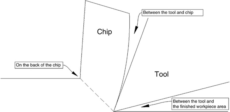
Cutting fluids can be applied primarily in one of three areas (directions) in the high-speed orthogonal cutting. It can be applied on the back of the chip. This method, according to Taylor, can increase tool life up to 40%. In addition, cutting fluids can be applied on the area between the tool and the finished workpiece. This method is useful for heavy cuts. With last method, cutting fluids are applied between the tool and the chip. This method has less support than the other two even though it looks better for cooling the buildup chips area. Many researchers say that the best direction for cooling is in the direction of the tool, which is between the tool and the finished area. Figure 9.10 illustrates the possibilities [34].
In modern industry, cutting fluid can be applied by cryogenic cooling. This method focuses on liquid nitrogen sprayed with two nozzles. Although environmentally friendly, this method is quite dangerous for the operator. Depending on the workpiece material and other parameters, the cryogenic cooling system can reduce the temperature by 34% and nearly 30% in cutting forces. This method sometimes uses CO2 instead of N2.
The increase of cutting with environmentally friendly operation guided some researchers to a new method called dry machining. In this method, no cutting fluids are presented. However, this method is limited to certain materials, and swarf control can be a problem. Some solutions were offered, but still the limitations exist [34].
Fluid application is accomplished by different methods including pouring the fluid, spraying it, or using high-velocity or low-velocity nozzles [8].
Conditioning
Because the grinding wheel will experience different kinds of wear during operation, we try to minimize wear by applying conditioning operations. Some of the operations are performed before starting the grinding process, and some are applied after the process proceeds. The operations that occur before the grinding process are called preparation and include ringing, mounting, and balancing. Other conditioning processes include cleaning-up, trueing, and dressing [23].
Ringing restores the integrity of the surface of the grinding wheel. The mounting process clamps and unclamps both the wheel and the workpiece to the grinding machine. Balancing makes sure that the wheel does not have any extra weight in any part of it that could generate a moment of inertia. The balancing process is especially recommended for new wheels [23].
Conventional Dressing
Dressing conditions the worn grains, especially grains that have attritious wear and dull grains. With conditioning, the grains gain new sharp edges, which increase their efficiency. Dressing is also applied when the wheel has loading. Loading occurs when part of the material removed sticks into the wheel affecting its accuracy, surface finish quality, and the heat generated during grinding. Loading usually happens from grinding soft materials or when grinding wheel type and material to be ground are not compatible. The dressing operation is performed using a hard diamond-point or diamond-cluster tool to remove a thin layer of the grinding wheel by traveling across the wheel while rotating. The diamond used in the dressing tool can be one of many types including the natural diamond (ND), broken natural diamond, synthetic diamond (SD), synthetic monocrystalline diamond (MCD), diamond chemical vapor deposition (CVD), and polycrystalline diamond (PCD) [23].
When a grinding wheel becomes dull or when it is loaded, it should be dressed by one of the dressing methods. The conventional method uses a diamond point or cluster dresser that travels across the wheel while the wheel is rotating, with a feed rate of Fd. The active area of the dresser width is dww. Because dressing plays a major role in the grinding operation, we can estimate the influence by calculating the overlap factor:
OLf=dwwFd
 (9.51)
Increasing the overlap factor will decrease the removal rate, but will give better roughness [61].
If the wheel is typically used in wet grinding, wet dressing is required. However, if the wheel is used in dry grinding, dry dressing is recommended. Dressing hard wheels requires different methods including a set of star-shaped steel disks or one of the nonconventional techniques. Moreover, dressing metal-bonded diamond wheels require the use of one of the nonconventional technologies. The first contact of the dressing with the wheel is extremely important. Therefore, advanced methods are used, including acoustic-emission sensors, vibration sensors, and power monitors. Nowadays, the dressing can take place during grinding to keep the wheel in good shape continuously by using computerized machines that monitor the condition of the wheel and act accordingly [2].
Trueing is used when the wheel loses its round shape. The process will return the wheel to its original round shape. It is necessary to perform trueing if the wheel has been balanced. For hard wheels, both dressing and trueing can be performed together in one operation. Nonetheless, trueing and dressing soft wheels need to be done separately. These operations are called conventional technologies [2].
In addition to the conventional operations of wheel conditioning, several nonconventional technologies for wheel conditioning enhance the wheel condition and involve the wheel in electrical, chemical, or physical operations.
Nonconventional Dressing Technologies
Many nonconventional techniques have been discovered to enhance the grinding process. The nonconventional technologies include many types, such as electrodischarge dressing (EDD), laser dressing, electrochemical dressing, and electrolytic in-process dressing (ELID). These processes may take place during the grinding process and do not necessitate stopping the operation. Moreover, the nonconventional operations combine both trueing and dressing at the same time [23].
Conventional grinding wheel dressing using a diamond dresser is purely mechanical, but is not efficient because it does not give a precise dressing and because it has a low-life dresser due to its high wear, especially in dressing superabrasive wheels. Other dressing methods such as electric spark eroding are more precise and efficient. Still, these processes are more costly due to the need for extra equipments, and the complexity of the process makes it difficult to be extensively used [6].
Laser Trueing and Dressing
Laser trueing and dressing was first introduced on CBN wheels by Westkamper. The idea is to use laser irradiation on the grinding wheel, which will soften the bond of the wheel. Then, it can be easily removed by a regular dresser. However, this operation has a huge risk of thermal or grit damages including graphitization of the diamond grains. Also, in the case of metal grinding wheels, this process could cause bond resolidification, in addition to the high initial cost of the laser dresser. Using an Nd:YAG laser dressing has reportedly eliminated these problems [52].
Electrodischarge Dressing
Electrodischarge dressing (EDD) can eliminate the runout trueing. Several improvements of the process have been discovered including electrocontact discharge dressing (ECDD) and dry electrodischarge dressing (dry-EDD). In the ECDD process, two electrodes are used in contact with the grinding wheel to help reduce thermal erosion. Dry-EDD uses one electrode with direct contact with the grinding wheel. However, graphitization has been reported with these methods [52].
Electrochemical Dressing
Electrochemical discharge machining (ECDM) was introduced after the foundation of ELID dressing. They exhibit similar outcomes. Some researchers have reported the creation of the oxide layer by using two electrodes with AC power supply [52].
9.3. Kinematics of the ELID grinding with lapping kinematics
The study will be conducted on the Melchiorre Machine (210-3P). This machine has two lower wheels and one upper spindle. Because this experiment is for a single-side grinding, some modifications needed to be implemented.
Trajectory
Part of the research is to understand the path the grain of the grinding wheel. In order to check an arbitrary point on the workpiece, we need to draw the trajectory of these points relative to both the workpiece and the grains on the grinding wheel. We can calculate its position by calculating its absolute coordinates and its relative coordinates as a function of time. In the present project, both the grinding wheel and spindle are rotating at different speeds and directions. Taking each case separately will ease the understanding of the final trajectory. The dimensions of the grinding wheel used are 211 mm OD and 113 mm ID with a thickness of 39 mm. Figure 9.11 shows the dimensions.

Figure 9.11 Grinding wheel dimensions
In the first case, the grinding wheel rotates while the spindle is stationary. The movement of the workpiece is constant at the lines, meaning that the movement will make parallel circles for the points on the workpiece at the grinding wheel (see Figure 9.12). Consequently, however, the grinding process speed will be unequal at each point of the workpiece. Points that are close to the center of the grinding wheel encounter slower grinding speed than the outward points.
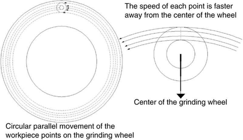
Figure 9.12 Trajectory with wheel motion only
In the case of a spindle rotation with no grinding wheel rotation, the movement on the grinding wheel will be parallel circles. Each point will rotate with different speed. For the workpiece itself, the same difference in speed for each point – as the points get closer to the center of the spindle – rotate at a significantly slower speed than that of the points away from it (see Figure 9.13).
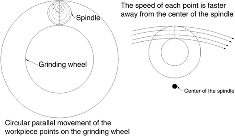
Figure 9.13 Trajectory with spindle motion only
In this project, the two rotations are presented at different speeds that give different profiles. In the article “Influence of Kinematics on the Face Grinding Process on Lapping Machine,” the authors investigated the double-sided flat grinding on lapping machine trajectory and path influences on the results. The examination showed that different paths with different grinding wheel and spindle speed ratios can significantly affect the roughness, flatness, and material removal rate. In this analysis, the better the roughness, the better the flatness, and the lower the material removal rate. The process can be applied in the opposite manner [62]. In the present project, each wheel and spindle speed combinations creates a unique grinding path. For the three wheel speeds and the three spindle speeds used in the project, we have a total combination of nine different trajectories. Each of these nine combinations is performed on three different eccentricities, totalling 27 runs. These runs follow three main patterns from the three different wheel speed ratios. For example, the trajectory while using the wheel speed ratio 1/2 will have two sides, and the trajectory while using the wheel speed ratio 1/4 will have four sides. Basically, the smaller the wheel speed ratio, the greater the tendency for the trajectory to have more circular shapes. The bigger ratios give more of an ellipse shape. This shape shifts the rotation while in operation to cover the wheel area for better wheel-wear balance. Using different eccentricities affects the trajectory by the amount the workpiece is covering the grinding wheel. For example, while using the eccentricity 17 mm, the whole grinding wheel is covered. However, using the eccentricity 9 mm will force the workpieces to cover only the internal portion of the grinding wheel. Figure 9.14 illustrates the influence of the eccentricity and wheel speed ratio.

Figure 9.14 The influence of the eccentricity and wheel speed ratio
These unique movements enables a more efficient grinding process and have a higher material removal rate due to the nonstop change of direction of the grains on the workpiece. According to previous research done on a surface scratching of a brittle material, the material removal rate from passing the abrasive grain twice at the same spot is small and considered inefficient and a waste of time and vitality [32].
The experimental variables are presented in Table 9.1. Other parameters are kept fixed for the current experiment and will be considered for evaluation in future experiments. These parameters are the following:
1. The output parameters of the ELID DC electrical power source are 72.4 V, 2 μs.
Table 9.1
Experimental Variables
| Spindle speed | ||||||||
| 150 rpm | 175 rpm | 200 rpm | ||||||
| Wheel speed | Wheel speed | Wheel speed | ||||||
| 75 rpm | 38 rpm | 19 rpm | 88 rpm | 44 rpm | 22 rpm | 100 rpm | 50 rpm | 25 rpm |
| Force | ||||||||
| 101.04 N | 148.13 N | 187.37 N | ||||||
| Eccentricity | ||||||||
| 17 mm | 13 mm | 9 mm | ||||||

2. Grinding wheel outer diameter is 211 mm, and the inner diameter is 114 mm.
3. Workpiece outer diameter is 13 mm, with an approximate initial height of 13 mm.
4. Coolant fluid is TRIM C270E with 5% concentration.
5. The gap between the electrode and the grinding wheel is fixed at 0.2 mm.
9.4. Modifications, preparations, and setup
The upper wheel (spindle) will be used to hold the workpiece. Three workpiece holders were designed with different eccentricities, including 17, 13, and 9 mm. These workpiece holders will be mounted one by one with three screws at the spindle cover position. Each workpiece holder is holding three workpieces at the same time, each using one screw. The benefit of this approach is to ensure that the workpieces are in a flat position with the grinding wheel because a flat plane needs three points to be defined. Also, machining three workpieces at once can ensure better results by reducing the error percentage. Figure 9.15 shows the workpiece holders with different eccentricities. The workpiece holders were designed and manufactured at the University of Toledo labs.
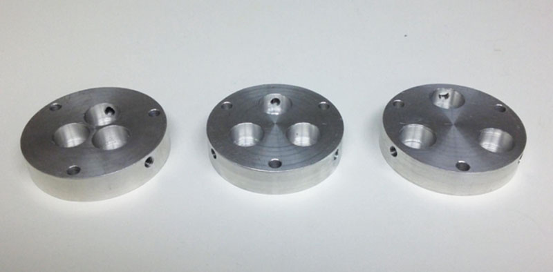
Figure 9.15 Workpiece holders from the left: 9, 13, 17 mm
Moreover, an electrode made out of stainless steel was manufactured in the lap to cover one-sixth of the grinding wheel abrasives area, and it is wider than the wheel on each side by 2 mm. The electrode is mounted using an electrical insulated material (Figure 9.16) on the outer ring of the machine, leaving a gap between the electrode and the grinding wheel of 0.1–0.3 mm. The outer ring on which the electrode is mounted rests on an elevation system that was built in the lab (Figure 9.17). By rotating the screw on the elevation system, the gap between the electrode and the grinding wheel can be controlled with great precision (Figures 9.18 and 9.19).
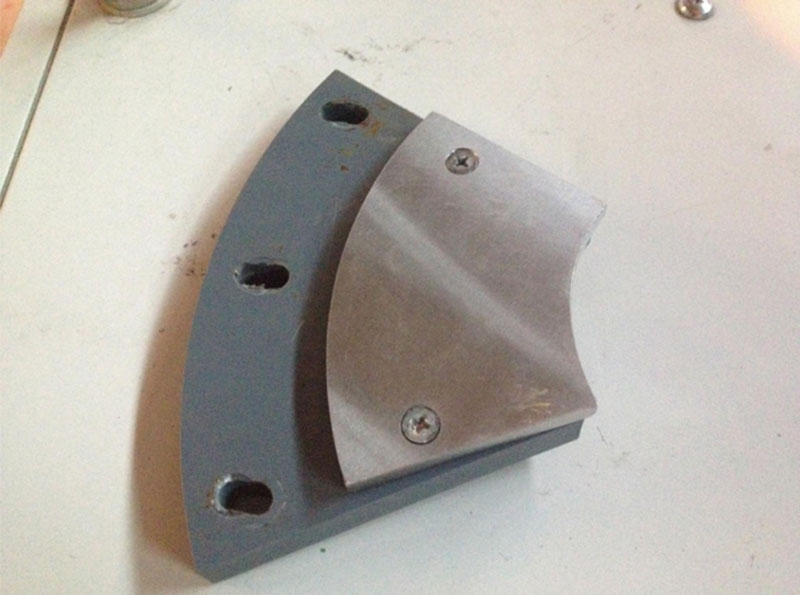
Figure 9.16 The electrode and the insulation material
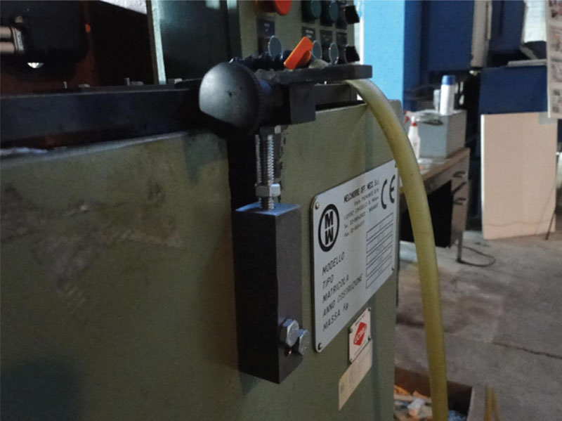
Figure 9.17 Elevation system
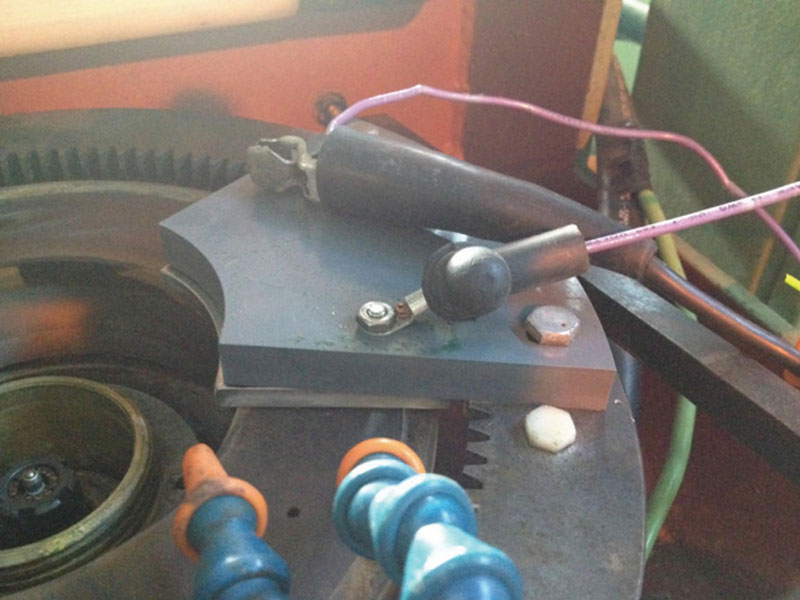
Figure 9.18 Electrode connected
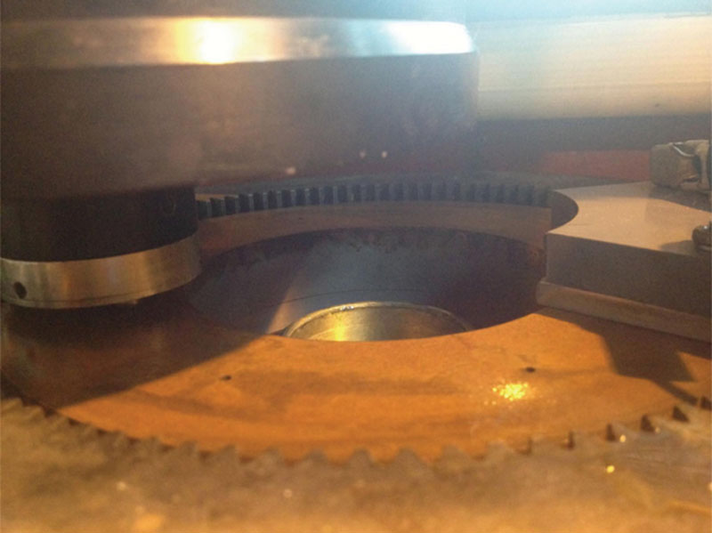
Figure 9.19 Complete systems running
Auxiliary Devices for the Experiment
Performing ELID grinding requires a number of external devices to support executing the process. These devices include the following:
ELID DC Electrical Source Machine
The electrical DC current required for ELID operation is being provided by the ELID machine in Figure 9.20. The electrical parameters of a Fuji Electric interrupting capacity system (EA33, F55068734) vary from 10 to 100 square-wave volts, 5–50 amps peak current, and 2–7 μs pulse width for both on-time and off-time [58].
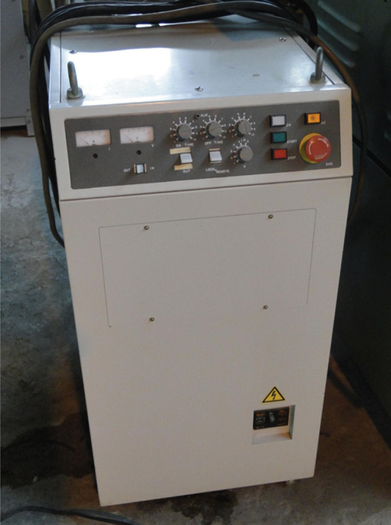
Figure 9.20 ELID electrical DC source
Coolant Pump
The coolant pump used in the experiment is a small submersible pump made by Little Giant Pump Co. (Franklin Electric) with epoxy-coated cast aluminum housing model (1-AA-18) with a horsepower of 1/200, 1.1 amps, and 70 W.
Measuring Systems
Two main properties are to be measured and discussed before and after each of the grinding operation cycles. The first property is the roughness of the workpieces. In the present project, only Ra is being measured. The first set of measurements during the testing of wheel mesh size #400 was collected by the Pocket Surf III measuring system. Smaller grain-size wheels (#1000, #2000) will have an additional measuring step. This step is to measure the final product workpieces using the Zygo machine (in this case, the NewView 5000 OMP-0423H by Zygo Corporation). The Zygo is a three-dimensional analyzer that provides graphic images and high-resolution numerical analysis to precisely illustrate the surface structure of test workpieces. Not only can it give a precise roughness, but it can also provide a 3D simulation graph or oblique 3D plot, surface image or an actual picture of the surface of the workpiece, 2D plane section, and flatness. The Zygo gives an option of choosing a line on the plane and evaluates it individually, in addition to many other features.
The second property to be tested is the material removal rate (MRR). This test can be done by measuring the weight of the workpiece before and after the grinding operation. The difference in weight will provide the weight of the material removed. Dividing that weight by the density and time gives the volume of the material removed per minute. Weight measuring is done using an electronic scale from A&D Company, limited model HR120.
Grinding Wheels with ELID Specifications
The main characteristic of the wheel used for ELID concentrates on the bond. This bond has to be electrically conductive. Thus, metal-bonded or metal-resin–bonded wheels are used for ELID. The metal part on the grinding wheels is usually made of cast iron for metal-bonded wheels and copper for metal-resin–bonded grinding wheels. Sometimes, a small amount of cobalt is added to the mixture [32]. In addition, the grains are fine and ultrafine superabrasive grains, such as diamond or cubic boron nitride (CBN) superabrasives. In the project, a metal-bond diamond superabrasive flat grinding wheel is used with different grades. The outer diameter of the wheel is about 210 mm and the inner diameter is about 113 mm.
Workpiece
Ceramics are brittle, have low electrical conductivity and intermediate density, but possess a high melting point. The workpiece used in this project is cylindrical shape rollers for ball bearings made out of silicon carbide (SiC),with a diameter of 13 mm and a height of about 13 mm. The silicon carbide used with a density of 3.21 g/cm3, and a hardness of 2800 kg/mm2, which is about 25 GPa on Vickers hardness. The melting point is at a temperature of 2730°C (4946°F), the flexure strength (bending strength) is about 490–550 MPa, and Young’s modulus is 392 GPa [62,63].
The Coolant Fluid
The coolant fluid used has a high pH. This fluid should be supplied at a rate of 20–30 L/min, and diluted in water to at least 1:50 [64]. In the present project, TRIM C270E is the coolant fluid used, provided by Master Chemical Cooperation. This coolant has a pH of 9 and a viscosity of 1.51 MPa. It will be used with a concentration of about 5%, and will be supplied in a way that a film of the coolant will be always covering the metal grinding wheel.
ELID Grinding Steps
In the present project, ED-trueing is skipped and the predressing is performed initially at a low grinding wheel speed. At the beginning of the predressing process, the voltage was low and the current was high. During the predressing stage, the current decreased and the voltage increased due to the accumulation of the oxide layer. Figure 9.21 illustrates the current-voltage electrical behavior during the predressing process.
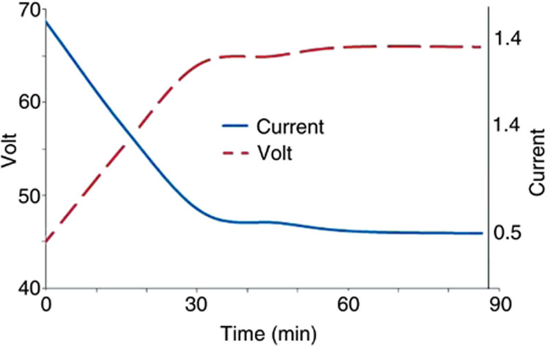
Figure 9.21 Electrical behavior during predressing process
9.5. Results
Analysis of Wheel #400 Data
After collecting the data, they are analyzed with Minitab software. In the real project, the wheel speed was a fraction of the spindle speed, which led to a different wheel speed at each spindle speed run. Therefore, wheel speed ratio was used as a variable on the factorial design calculations. Four inspections have been conducted. The two main measurements collected during the experiment were the roughness and the material removal rate. Two of the four examinations were for each measurement. The first one included all the variables during the periods of measurements. The second one is taking the results for all the variables with the final results after the whole period of 30 min. Hence, the time will be constant.
For the first set, the variables used in the analysis were:
1. Spindle speed (3 factors including 150, 175, 200 rpm)
2. Wheel speed ratio (3 factors including 1/2, 1/4, 1/8)
3. Load (3 factors including 10.3, 15.1, 19.1 kg)
4. Eccentricity (3 factors including 17, 13, 9 mm)
5. Time (4 factors including 5, 10, 20, 30 min)
For the second set, the variables used in the analysis were the same, except that the time was constant, giving a full factorial with four variables instead of five (the first four above).
Both sets were conducted on the roughness (Ra) and the material removal rate (MRR).
Roughness with Time for Wheel #400
Minitab results for the roughness with the five factors follow:
Multilevel Factorial Design
| Factors | 5 | Replicates | 1 |
| Base runs | 405 | Total runs | 405 |
| Base blocks | 1 | Total blocks | 1 |

Number of levels: 3, 3, 3, 3, 5.
General Linear Model: Roughness (R Versus Spindle Speed, Wheel Speed Ratio, Eccentricity, Force, Time)
| Factor | Type | Levels | Values |
| Spindle speed (rpm) | Fixed | 3 | 150, 175, 200 |
| Wheel speed ratio | Fixed | 3 | 0.125, 0.250, 0.500 |
| Eccentricity (mm) | Fixed | 3 | 9, 13, 17 |
| Force (N) | Fixed | 3 | 101.04, 148.13, 187.37 |
| Time (min) | Fixed | 5 | 0, 5, 10, 20, 30 |

Analysis of Variance for Roughness (Ra), Using Adjusted SS for Tests
| Source | DF | Seq. SS | Adj. SS | Adj. MS | F | P |
| Spindle speed (rpm) | 2 | 0.005816 | 0.005816 | 0.002908 | 21.63 | 0.00 |
| Wheel speed Ratio | 2 | 0.000127 | 0.000127 | 0.000063 | 0.47 | 0.625 |
| Eccentricity (mm) | 2 | 0.013118 | 0.013118 | 0.006559 | 48.78 | 0.000 |
| Force (N) | 2 | 0.019236 | 0.019236 | 0.009618 | 71.52 | 0.000 |
| Time (min) | 4 | 0.127702 | 0.127702 | 0.031926 | 237.41 | 0.000 |
| Error | 392 | 0.052714 | 0.052714 | 0.000134 | ||
| Total | 404 | 0.218713 |
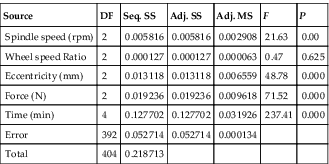
S = 0.0115963, R2 = 75.90%, R2 (adj.) = 75.16%.
Unusual Observations for Roughness (Ra)
| Roughness | |||||
| Obs (Ra) | Fit | SE Fit | Residual | St. residual | |
| 4 | 0.143000 | 0.111385 | 0.002078 | 0.031615 | 2.77 R |
| 31 | 0.153000 | 0.120667 | 0.002078 | 0.032333 | 2.83 R |
| 53 | 0.130000 | 0.095205 | 0.002078 | 0.034795 | 3.05 R |
| 107 | 0.150000 | 0.119504 | 0.002078 | 0.030496 | 2.67 R |
| 111 | 0.143000 | 0.118017 | 0.002078 | 0.024983 | 2.19 R |
| 114 | 0.153000 | 0.121600 | 0.002078 | 0.031400 | 2.75 R |
| 115 | 0.167000 | 0.122277 | 0.002078 | 0.044723 | 3.92 R |
| 118 | 0.183000 | 0.132548 | 0.002078 | 0.050452 | 4.42 R |
| 141 | 0.083000 | 0.106941 | 0.002078 | −0.023941 | −2.10 R |
| 185 | 0.087000 | 0.111496 | 0.002078 | −0.024496 | −2.15 R |
| 206 | 0.127000 | 0.103319 | 0.002078 | 0.023681 | 2.08 R |
| 220 | 0.150000 | 0.123311 | 0.002078 | 0.026689 | 2.34 R |
| 306 | 0.153000 | 0.115941 | 0.002078 | 0.037059 | 3.25 R |
| 320 | 0.137000 | 0.112363 | 0.002078 | 0.024637 | 2.16 R |
| 368 | 0.150000 | 0.125864 | 0.002078 | 0.024136 | 2.12 R |
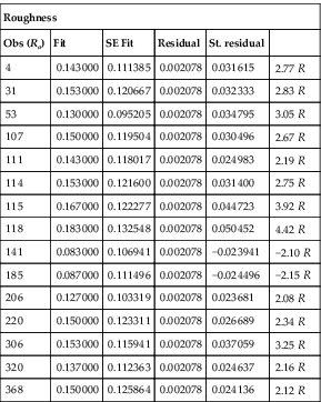
R denotes an observation with a large standardized residual.
Roughness with Constant Time for Wheel #400
Multilevel Factorial Design
| Factors | 4 | Replicates | 1 |
| Base runs | 81 | Total runs | 81 |
| Base blocks | 1 | Total blocks | 1 |
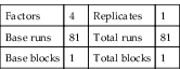
Number of levels: 3, 3, 3, 3.
General Linear Model: Roughness (R Versus Spindle Speed, Wheel Speed Ratio, Eccentricity, Force)
| Factor | Type | Levels | Values |
| Spindle speed (rpm) | Fixed | 3 | 150, 175, 200 |
| Wheel speed ratio | Fixed | 3 | 0.125, 0.250, 0.500 |
| Eccentricity (mm) | Fixed | 3 | 9, 13, 17 |
| Force (N) | Fixed | 3 | 101.04, 148.13, 187.37 |

Analysis of Variance for Roughness (Ra), using Adjusted SS for Tests
| Source | DF | Seq. SS | Adj. SS | Adj. MS | F | P |
| Spindle speed (rpm) | 2 | 0.0010963 | 0.0010963 | 0.0005481 | 7.71 | 0.001 |
| Wheel speed ratio | 2 | 0.0002721 | 0.0002721 | 0.0001360 | 1.91 | 0.155 |
| Eccentricity (mm) | 2 | 0.0030250 | 0.0030250 | 0.0015125 | 21.28 | 0.000 |
| Force (N) | 2 | 0.0033087 | 0.0033087 | 0.0016544 | 23.27 | 0.000 |
| Error | 72 | 0.0051179 | 0.0051179 | 0.0000711 | ||
| Total | 80 | 0.0128200 |

S = 0.00843103, R2 = 60.08%, R2 (adj.) = 55.64%.
Unusual Observations for Roughness (Ra)
| Roughness | |||||
| Obs (Ra) | Fit | SE Fit | Residual | St. Residual | |
| 34 | 0.083000 | 0.101111 | 0.002810 | −0.018111 | −2.28 R |
| 64 | 0.130000 | 0.101963 | 0.002810 | 0.028037 | 3.53 R |
| 77 | 0.137000 | 0.116111 | 0.002810 | 0.020889 | 2.63 R |
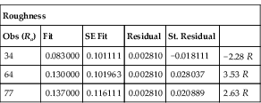
R denotes an observation with a large standardized residual.
MRR with Time for Wheel #400
General Linear Model: MRR (mm3/min Versus Spindle Speed, Wheel Speed Ratio, Eccentricity, Force, Time)
| Factor | Type | Levels | Values |
| Spindle speed (rpm) | Fixed | 3 | 150, 175, 200 |
| Wheel speed ratio | Fixed | 3 | 0.125, 0.250, 0.500 |
| Eccentricity (mm) | Fixed | 3 | 9, 13, 17 |
| Force (N) | Fixed | 3 | 101.04, 148.13, 187.37 |
| Time (min) | Fixed | 4 | 5, 10, 20, 30 |

Analysis of Variance for MRR (mm3/min), using Adjusted SS for Tests
| Source | DF | Seq. SS | Adj. SS | Adj. MS | F | P |
| Spindle speed (rpm) | 2 | 0.00737 | 0.00737 | 0.00368 | 0.82 | 0.440 |
| Wheel speed Ratio | 2 | 2.02283 | 2.02283 | 1.01142 | 226.22 | 0.000 |
| Eccentricity (mm) | 2 | 2.46943 | 2.46943 | 1.23472 | 276.16 | 0.000 |
| Force (N) | 2 | 0.00445 | 0.00445 | 0.00222 | 0.50 | 0.609 |
| Time (min) | 3 | 0.18830 | 0.18830 | 0.06277 | 14.04 | 0.000 |
| Error | 312 | 1.39495 | 1.39495 | 0.00447 | ||
| Total | 323 | 6.08732 |

S = 0.0668654, R2 = 77.08%, R2 (adj.) = 76.28%.
Unusual Observations for MRR (mm3/min)
| MRR | |||||
| Obs. | (mm3/min) | Fit | SE Fit | Residual | St. Residual |
| 5 | 0.150000 | 0.409691 | 0.012868 | −0.259691 | −3.96 R |
| 18 | 0.520000 | 0.310895 | 0.012868 | 0.209105 | 3.19 R |
| 69 | 0.710000 | 0.485340 | 0.012868 | 0.224660 | 3.42 R |
| 123 | 0.690000 | 0.482747 | 0.012868 | 0.207253 | 3.16 R |
| 135 | 0.580000 | 0.427654 | 0.012868 | 0.152346 | 2.32 R |
| 156 | 0.560000 | 0.375000 | 0.012868 | 0.185000 | 2.82 R |
| 167 | 0.240000 | 0.380802 | 0.012868 | −0.140802 | −2.15 R |
| 187 | 0.560000 | 0.412469 | 0.012868 | 0.147531 | 2.25 R |
| 204 | 0.710000 | 0.533117 | 0.012868 | 0.176883 | 2.70 R |
| 206 | 0.370000 | 0.236636 | 0.012868 | 0.133364 | 2.03 R |
| 215 | 0.550000 | 0.371728 | 0.012868 | 0.178272 | 2.72 R |
| 216 | 0.210000 | 0.433951 | 0.012868 | −0.223951 | −3.41 R |
| 228 | 0.580000 | 0.430247 | 0.012868 | 0.149753 | 2.28 R |
| 259 | 0.500000 | 0.324043 | 0.012868 | 0.175957 | 2.68 R |
| 266 | 0.240000 | 0.380370 | 0.012868 | −0.140370 | −2.14 R |
| 293 | 0.540000 | 0.403395 | 0.012868 | 0.136605 | 2.08 R |

R denotes an observation with a large standardized residual.
MRR with Constant Time for Wheel #400
General Linear Model: MRR (mm3/min Versus Spindle Speed, Wheel Speed Ratio, Eccentricity, Force)
| Factor | Type | Levels | Values |
| Spindle speed (rpm) | Fixed | 3 | 150, 175, 200 |
| Wheel speed ratio | Fixed | 3 | 0.125, 0.250, 0.500 |
| Eccentricity (mm) | Fixed | 3 | 9, 13, 17 |
| Force (N) | Fixed | 3 | 101.04, 148.13, 187.37 |
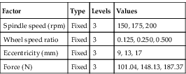
Analysis of Variance for MRR (mm3/min), using Adjusted SS for Tests
| Source | DF | Seq. SS | Adj. SS | Adj. MS | F | P |
| Spindle speed (rpm) | 2 | 0.00281 | 0.00281 | 0.00140 | 0.77 | 0.469 |
| Wheel speed ratio | 2 | 0.49903 | 0.49903 | 0.24951 | 136.17 | 0.000 |
| Eccentricity (mm) | 2 | 0.62327 | 0.62327 | 0.31163 | 170.07 | 0.000 |
| Force (N) | 2 | 0.00005 | 0.00005 | 0.00003 | 0.01 | 0.986 |
| Error | 72 | 0.13193 | 0.13193 | 0.00183 | ||
| Total | 80 | 1.25709 |
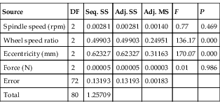
S = 0.0428066, R2 = 89.50%, R2 (adj.) = 88.34%.
Unusual Observations for MRR (mm3/min)
| MRR | |||||
| Obs. | (mm3/min) | Fit | SE Fit | Residual | St. Residual |
| 19 | 0.630000 | 0.510741 | 0.014269 | 0.119259 | 2.95 R |
| 47 | 0.600000 | 0.497037 | 0.014269 | 0.102963 | 2.55 R |
| 64 | 0.600000 | 0.509259 | 0.014269 | 0.090741 | 2.25 R |
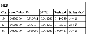
R denotes an observation with a large standardized residual.
As a conclusion for the Minitab results above, a minor randomization violation arose because of some assumptions. Lack of fit and errors are due to the assumption that no factor interaction occurs. Even though few of the two factor interactions were relative by having some means of high p-value, the model fits fine without them. Three-factor interaction and higher were completely insignificant.
Model Calculations for Wheel #400
The main goal of this section is to find exponents for the proposed model for future responses predictions.
Roughness Model for Wheel #400
The equation suggested is:
Ra=C.Vα.Fβ.eγ
After running the experiment, we want to fit this model in order to predict future results. The model has four unknowns that require four equations to solve. However, the current experiment provides multiple equations. Therefore, a special method should be applied on the data for the optimum approximation of the data. Multiple methods have been considered including least square method and multicorrelation theory. The last method is the most applicable method because it is designed to find a number of constants for a larger number of equations [65]. To find these exponents using the multicorrelation theory, apply the logarithm for equation (9.52):
log(Ra)=log(C.Vα.Fβ.eγ)
Because:
logb(bx)=xlogb(b)=x
and (9.55)
logb(M×N)=logb(M)+logb(N)
then:
log(Ra)=log(C)+α.log(V)+β.log(F)+γ.log(e)
With 81 experimental runs made, 81 equations can be written. Using the multicorrelation theory, these equations can be written in four equations only as the following:
∑81i=1log(Ra)=nlog(C)+α∑81i=1log(V)+β∑81i=1log(F)+γ∑81i=1log(e)
 (9.57)
The other three equations are related to (V, F, and e) respectively:
⇒∑81i=1log(V)log(Ra)=log(C)∑81i=1log(V)+α∑81i=1[log(V)]2+β∑81i=1log(V)log(F)+γ∑81i=1log(V)log(e)
 (9.58)
⇒∑81i=1log(F)log(Ra)=log(C)∑81i=1log(F)+α∑81i=1log(V)log(F)+β∑81i=1[log(F)]2+γ∑81i=1log(F)log(e)
 (9.59)
⇒∑81i=1log(e)log(Ra)=log(C)∑81i=1log(e)+α∑81i=1log(V)log(e)+β∑81i=1log(F)log(e)+γ∑81i=1[log(e)]2
 (9.60)
The sum of all 81 equations led to the following four equations:
−83.552=81log(C)+181.4443α+174.0916β+89.0631γ−187.22046=181.4443log(C)+406.65596α+389.97β+199.506γ−179.8066=174.0916log(C)+389.97α+375.161β+191.42γ−91.64=89.0631log(C)+199.506α+191.42β+98.967γ
 (9.61)
Four equations with four unknowns, this system of equations can be solved by MATLAB. MATLAB solution is:
≫A=[81181.4443174.091689.0631 181.4443406.65596389.97199.506 174.0916389.97375.161191.42 89.0631199.506191.4298.967]

B=[−83.552 −187.22046 −179.8066 −91.64]
X=inv(A)×B
X= −0.1295 −0.2869 −0.2334 0.2204
This gives log(C) = –0.1295
α=−0.2869β=−0.2334γ=0.2204
Therefore, the results are:
⇒C=0.7422,α=−0.2869,β=−0.2334,γ=0.2204
The final model is:
Ra=0.7422 V−0.2869 F−0.2334 e0.2204 OrRa=0.7422e0.2204V0.2869F0.2334
 (9.62)
Material Removal Rate Model for Wheel #400
Similarly, the material removal rate model is:
MRR=C.Vα.Fβ.eγ
The procedure is the same and the constants can be achieved in the following steps:
log(MRR)=log(C.Vα.Fβ.eγ)
log(MRR)=log(C)+α.log(V)+β.log(F)+γ.log(e)
The summation of the 81 equations using the multicorrelation theory is:
∑81i=1log(MRR)=nlog(C)+α∑81i=1log(V)+β∑81i=1log(F)+γ∑81i=1log(e)
 (9.66)
The other three equations are related to (V, F, and e) respectively:
⇒∑81i=1log(V)log(MRR)=log(C)∑81i=1log(V)+α∑81i=1[log(V)]2+β∑81i=1log(V)log(F)+γ∑81i=1log(V)log(e)
 (9.67)
⇒∑81i=1log(F)log(MRR)=log(C)∑81i=1log(F)+α∑81i=1log(V)log(F)+β∑81i=1[log(F)]2+γ∑81i=1log(F)log(e)
 (9.68)
⇒∑81i=1log(e)log(MRR)=log(C)∑81i=1log(e)+α∑81i=1log(V)log(e)+β∑81i=1log(F)log(e)+γ∑81i=1[log(e)]2
 (9.69)
The four equations are:
−46.276=81log(C)−48.767α+174.092β+89.0631γ30.191=−48.767log(C)+34.254α−104.814β−53.621γ−99.445=174.092log(C)−104.814α+375.161β+191.422γ−49.658=89.0631log(C)−53.621α+191.422β+98.967γ
 (9.70)
Four equations with four unknowns, this system of equations can be solved. MATLAB solution is:
A =[81−48.767174.09289.0631 −48.76734.254−104.814−53.621 174.092−104.814375.161191.422 89.0631−53.621191.42298.967]
B=[−46.27630.191−99.445−49.658]
x=inv(A)×B
x=−1.61420.47600.01531.1793
This gives log(C) = –1.6142α=0.4760β=0.0153γ=1.1793
Therefore, the results are:
⇒C=0.024331,α=0.476,β=0.0153,γ=1.1793
The final model is:
MRR=0.024311 V0.476r F0.0153 e1.1793
The speed used for the roughness modeling is not the same as the material removal rate model. In order for each model to have a high prediction capability, the factors should be significant. In other words, the factors used should be the factors that affect the response. Therefore, spindle speed was used for roughness modeling as (V), whereas wheel speed ratio (Vr) was used for material removal rate modeling.
..................Content has been hidden....................
You can't read the all page of ebook, please click here login for view all page.