Chapter 2. Storage Networks: Existing Designs

This chapter covers the following key topics:

• The Storage View of Multitier Designs: Offers a high-level description of the three-tier storage network from the point of view of a storage administrator.

• Types of Disk Drives: Discusses types of disk drives commonly used in enterprise networks, such as HDD SAS, HDD SATA, SAS SED, fibre channel, and SSDs.

• Disk Performance: Covers disk performance, which is affected by the type of drive and the server interconnect. Performance metrics such as transfer speed, throughput, latency, access times, and IOPS are described.

• RAID: Highlights different RAID systems, which offer a variety of data protection and faster I/O access.

• Storage Controllers: Describes the functions of storage controllers, such as fibre channel and iSCSI, inside hosts and storage arrays.

• Logical Unit Numbers: Explains how RAID systems are partitioned into logical unit numbers and volumes to hide the physical disk from the operating system.

• Logical Volume Manager: Describes how RAID systems are partitioned into volumes to hide the physical disk from the operating system.

• Block, File, and Object-Level Storage: Covers the different types of storage technologies and how various applications use them.

• Storage-to-ServerConnectivity: Discusses how storage connects to servers via direct-attached storage (DAS) or via the network using network-attached storage (NAS) and storage area networks (SANs). Describes SAN fibre channel and iSCSI addressing and switching and network security such as zoning and masking.

• Storage Efficiency Technologies: Distinguishes between storage efficiency technologies such as thin provisioning, types of snapshots, cloning, source- and target-based deduplication, inline and post-process deduplication, compression, storage encryption, storage tiering, and so on.

Although some of the information in this chapter might be familiar to information technology (IT) storage professionals, it might not be too obvious to those with a system software or data networking background. Evolution in the storage space is moving quickly, and storage professionals must keep up with the advances in technology. This chapter discusses some storage basics, such as the different types of drives, storage protocols, and storage functionality, which set the stage for more advanced topics in future chapters. Next, it examines the different types of drives and storage protocols.

The Storage View of Multitier Designs

When speaking with storage vendors, the whole data networking piece of the puzzle disappears and turns into a simple black box. As you saw in Chapter 1, “Data Networks: Existing Designs,” the black box has many knobs, and it can get complex, so do not take it lightly. With storage vendors, the focus turns to servers, storage controllers, file systems, disks, and backup. Convergence and hyperconvergence emerged to solve the complexities of storage performance and management. However, in doing so the traditional storage networking technologies are heading in the direction of data networking technologies with the adoption of Internet Protocol (IP) and Gigabit Ethernet (GE) networks. From a storage network view, the three tiers are the servers, the storage network, and the disks. Each tier has its share of interoperability and compatibility issues. This is mainly because server vendors had to deal with operating system compatibility issues with network interfaces and disk controllers, disk vendors went through many iterations to improve disk capacity and speeds, and storage networking vendors had to figure out how to deal with the multiple storage protocols like Fibre Channel, Network File System (NFS), and Internet Small Computer System Interface (iSCSI).

The server tier is composed of the servers that provide the processing and compute to run the different applications. The storage network tier is made up of storage switches such as fibre channel (FC) switches—or GE switches in the case of iSCSI or NFS. The storage disks tier contains the actual disks. Hyperconvergence attempts to combine all these tiers into one product that unites the compute, storage network, and disks, and integrates with the data network. Figure 2-1 shows the storage view of a multitier storage architecture and how it relates to the data networking view that was previously discussed. This is one type of storage application. Several others are discussed later in this chapter.

Notice that in the storage view of this example, servers are connected to the storage network via FC switches, and the switches are connected to storage arrays. Storage arrays contain storage controllers to handle the storage transactions and house the actual disks where the data exists. In the cases of iSCSI and NFS, the storage network tier is normally built with GE and 10 GE switches. Regardless of which technology is used for the storage protocols and storage networks, this adds extra layers of complexity to deal with. This is an area that hyperconvergence solves by collapsing the layers and by addressing the performance and management issues of converging data and storage traffic over a unified fabric.

Figure 2-1 Multitier Storage Architecture

To fully understand the issues with storage networks, you must start with the different types of disks and the challenges they have in access speeds and durability.

Types of Disk Drives

There are different types of disk drives: hard drives, solid-state drives, optical drives, tape drives, flash drives, and so on. Let’s examine a sample of the most typical drives that you encounter in data centers. Optical drives and tape drives are not discussed here.

Hard Disk Drives

Hard disk drives (HDDs) are the lowest cost drives on the market (ignoring tape drives). They are formed of platters that spin around a spindle, with information being read or written by changing the magnetic fields on the spinning platters. A read/write head hovering above the platter seeks the information from the platter. The platter is formed of tracks and sectors, as illustrated in Figure 2-2. The hard disk access time is one of the factors that affects the performance of the application. The access time is the total of the seek time, which is the time it takes the read/write head to move from one track to another, and the time it takes the head to reach the correct sector on the rotating platters. HDDs are cost effective, but they contribute to high access times, they consume a lot of power, and they are prone to failure just because they are mechanical devices.

Figure 2-2 Hard Disk Drive Tracks and Sectors

HDDs connect to other peripherals via different types of interfaces, including Serial Advanced Technology Attachment (SATA) and Serial Attached Small Computer System Interface (SAS). It is worth noting that although SATA and SAS are interfaces that connect different types of drives to the computer or server, the drives themselves are usually named SATA drives and SAS drives. Other types of drives are the FC drives. The decision to use SATA, SAS, or FC drives depends on price and performance.

SATA Drives

SATA drives are suited for applications that require less disk performance and less workload. The SATA platter speed is 7200 revolutions per minute (RPMs) as used on servers; older, lower platter speeds such as 5400 RPM drives are normally used on computers. A combination of high-performance SATA drives and controllers is used as a cost-effective solution in building server disk arrays. SATA drives use the Advanced Technology Attachment (ATA) command for data transfer.

SAS Drives

SAS drives are suited for applications that require higher disk performance and higher workload. The SAS platter speed is a maximum 15,000 RPM; 10,000 RPM disks are available as well. SAS capacity is much smaller and more expensive per gigabyte than SATA drives. SAS drives are better suited for servers, especially at lower capacity requirements; however, for high-capacity requirements, the steep price of SAS might outweigh the performance benefits. Other networked storage solutions might be more suited. SAS drives use the SCSI command set. Both SAS drives and SATA drives can plug in a SAS backplane; SAS cannot plug in a SATA backplane.

SAS Self-Encrypting Drives

SAS self-encryption drives (SEDs) allow the automatic encryption and decryption of data by the disk controller. SED protects the data from theft and does not affect the performance of the application because the encryption and decryption are done in hardware. SAS SED drives are more expensive than regular SAS drives. SAS SED drives come as SAS SED HDDs or SAS SED SSDs.

FC Drives

Fibre channel (FC) drives are suited for enterprise server applications. They have similar performance to SAS drives but are more expensive. FC connectivity is via multimode fibre. Although FC drives have similar performance to SAS, most of the hard drives in the market continue to be SAS or a combination of SAS and SATA. FC leads as a connectivity method for storage area networks (SANs), and it carries the SCSI command set over the network. SAN connectivity is dominated by fibre channel, but the actual hard disks in SAN arrays are SASs.

Solid-State Drives

Unlike HDDs, solid-state drives (SSDs) have no motors, reading heads, or spinning platters; they are basically built with no moving parts. Early SSDs were built based on random access memory (RAM); however, the latest SSDs are based on flash memory. SSDs are a lot more expensive than HDDs and offer much higher performance because, unlike HDDs that rely on a moving head and spinning platter to read/write the information, SSDs rely on an embedded processor to store, retrieve, and erase data. SSDs have fewer capacities than HDDs, but next-generation SSDs keep increasing in capacity to compete with HDD capacity. SSDs like HDDs connect to peripherals via interfaces. SSDs connect to servers via a SATA interface, or SAS.

Disk Performance

Disk performance for reads and writes depends on factors such as the disk media itself—whether it is an HDD or an SSD—disk queue depth, and other factors such as the interconnect between the disk and the server. This section discusses factors that affect disk performance and the terminology used in the industry. Next, let’s examine transfer speeds in terms of throughput, latency, and input/output operations per second (IOPS).

Throughput or Transfer Speed

The transfer speed is essentially the rate at which data is transferred to and from the disk media in a certain period of time. Transfer speed is measured in megabytes per second (MBps) or gigabits per second (Gbps), keeping in mind that 1 Gigabit = 1000 Megabits, so 1 Gbps = 1000 / 8 = 125 MBps. Transfer speed is affected by the actual bus connecting the disk. There are different bus interconnects:

• SATA: SATA 1 has a 1.5 Gbps transfer speed, SATA 2 is at 3 Gbps, and SATA 3 is at 6 Gbps. So, for example, a 3 Gbps SATA 2 connection has a 3 × 1000 / 8 = 375 MBps transfer speed, and with overhead it decreases to 300 MBps. In contrast, a SATA 3 connection works at 6 Gbps or 6 × 1000 / 8 = 750 MBps transfer speed, and with overhead it decreases to 600 MBps.

• SAS: SAS 1 has a transfer speed of 3 Gbps, SAS 2 is 6 Gbps, SAS 3 is 12 Gbps, and SAS 4 is 22.5 Gbps.

Other interfaces are Peripheral Component Interconnect express (PCIe) and Non-Volatile Memory express (NVMe), which are described in Chapter 3, “Host Hardware Evolution.”

Access Time

Access time, discussed earlier, is the overall measure, normally in milliseconds, of the time it takes to start the data transfer operation. Because SSDs have no moving parts, they have much lower access times than HDDs. The access times depend on the vendors’ implementations. Typical access times for HDDs are in the 10-millisecond range or less, whereas access times of SSDs are in the 100 microsecond range or less, which is magnitudes faster. The SSD access times continue to decrease.

Latency and IOPS

Other performance indicators that enterprises and data centers designers rely on when looking at disk performance are latency and IOPS.

Latency is defined as the time it takes to complete an I/O operation. This differs whether you are looking at latency from a disk perspective or from a host/application perspective. If, for example, a disk can perform a single I/O operation in 10 ms, the latency from the disk perspective is 10 ms. But if two I/O operations arrive at the same time, the second operation must wait for the first to finish, and the total time for both I/Os to finish becomes 20 ms. Therefore, from an application perspective, the latency is 20 ms.

IOPS is the maximum number of I/O operations per second; an input operation is a write, and an output operation is a read. IOPS is measured as an integer number, such as 210 IOPS or 10,000 IOPS. IOPS are important in applications such as databases that handle a lot of I/O requests in small block sizes in a short time. So even though two disks might have the same capacity, the disk with the highest IOPS handles a lot more operations in a short amount of time. Different factors affect IOPS, including the access time for the disk to perform the operation and the queue depth. The queue depth refers to the outstanding I/O operations that a disk attempts to perform in parallel. This can offer a multiplying effect for increasing the IOPS. A host bus adapter (HBA) that supports a queue depth of 4 will have almost four times the IOPS as an HBA with a queue depth of 1. This, of course, depends on whether you are considering SSDs or HDDs. SSDs, for example, have multiple channels, where a larger queue depth translates in more I/O being done in parallel. With HDDs, the effect of queue depth is limited by the fact that spinning disks and moving heads constrain which operations can be done in parallel.

Another factor to consider when looking at IOPS is the I/O transfer size. Many operating systems and applications perform I/O operations in different block sizes. Some will do I/O with 4 KB block size; others will do it with 64 KB, and so on. A disk that can achieve 10,000 IOPS at 64 KB block size is more powerful than one that achieves the same IOPS at 4 KB block size.

IOPS in general has an inverse relationship with latency from an application perspective. Therefore, if an application calculates overall latency of 0.01 ms, the disk IOPS should be in the range of 1/0.01 = 100,000 IOPS.

SSD drives deliver far more IOPS than HDD SATA or SAS drives—normally in the tens and hundreds of thousands and even reaching a million IOPS, and especially in randomized data patterns and smaller block sizes. Other factors affecting performance for local disks are interface speeds, data being sequential or randomized, whether you are doing a read or a write operation, and the number of disks and the fault tolerance level in disk arrays.

Another factor that affects performance is how data is read or written on the disk. If you are reading or writing large files in large block sizes in a sequential fashion, there isn’t much movement of the disk head, so the access times are smaller. However, on the other extreme, if data is stored on the disk in small blocks and in a random fashion, the access times to read and write are much larger, which reduces performance. In random patterns, there are a lot of disk seeks with HDDs that reduce performance.

The performance of disks also depends on the disk interface, such as SATA and SAS. It is important that the I/O bandwidth resulting from the IOPS operations does not exceed the disk throughput or transfer speed; otherwise, the interface speed becomes the bottleneck. For example, an SSD disk handling 200,000 IOPS for 4 K (as in 4 KB) data blocks is actually transferring 200,000 × 4KB = 800,000 KBps, or 800 MBps. As you’ll recall, you calculated the theoretical transfer speed of a SATA 3 interface at 6 Gbps, or 750 MBps. So, at 200,000 IOPS, the I/O bandwidth that a disk can handle exceeds the interface’s theoretical limit, and the interface becomes a bottleneck. As such, it is important that faster IOPS be matched with faster interface speeds. On the other hand, IOPS are related to the number of disks in a redundant array of independent (or inexpensive) disks (RAID) system, as discussed next.

RAID

The RAID (Redundant Array of Independent Disks) system was created under the notion that multiple smaller and inexpensive disks have better performance than one large and expensive disk. This is because if multiple disks are doing read/write operations in parallel, data is accessed faster than with a single disk. This assumes data striping, which is equally dividing the data between the multiple disks. So, for example, if there are five blocks of data to be read on one large disk, the access time (time to move between tracks and reach a sector) is multiplied by 5. If five disks are doing the operation in parallel, there is one access time to read all data.

Other than performance, RAID systems offer a more reliable and available storage system to withstand failures of individual disks. As such, different RAID levels were created depending on the required balance between performance, reliability, and availability. Let’s look at some of the most popular RAID systems: RAID 0, 1, 1+0, and 0+1, 5, and 6.

RAID 0

RAID 0 combines all drives into one giant drive—mainly like a JBOD (just a bunch of disks)—however, it stripes (equally divides) the data across all disks. This striping improves the performance because all disks seek portions of the data at the same time. RAID 0 has no fault tolerance; if one disk fails, the whole data is lost. Notice in Figure 2-3a how equal-sized blocks B1, B2, B3 are equally striped on three disks.

RAID 1

RAID 1 offers disk mirroring. Say that a disk array has eight disks. Four of these disks are an exact duplicate of the others. From a performance level, read/write speeds are very good, and from a fault-tolerance level, if one disk fails, there is a ready mirror copy of that disk, so data is not lost. The disadvantage of RAID 1 is that half of the capacity is lost; therefore, 8 × 1 Terabyte (TB) drives actually give 4 TB of capacity. Notice in Figure 2-3b how data blocks B1, B2, and B3 are mirrored across two disks.

RAID 1+0

RAID 1+0 is a combination of a RAID 0 and a RAID 1 and requires a minimum of four disks. It is a stripe of mirrored set (stripe + mirror). RAID 0 stripes the data between different arrays, but RAID 1 mirrors the drives within the array. This is seen in Figure 2-4a. The advantage of RAID 1+0 is good read/write performance and the ability to protect against disk failure. Its disadvantage is that if a set of mirrored disks fails—for example, if both disk 1 and its mirror disk 2 fail in the same array—then the whole data ends up being lost. Add to this the fact that half of the capacity of the array is lost because of mirroring.

Figure 2-3 RAID 0, RAID 1 Example

Figure 2-4 RAID 1+0 (left) and RAID 0+1 (right) Examples

RAID 0+1

RAID 0+1 is a combination of RAID 1 and RAID 0. It is a mirror of a striped set (mirror + stripe). RAID 1 mirrors the data between arrays, whereas RAID 0 stripes the data between the drives of the same array. This is seen on the right side of Figure 2-4. The advantage of RAID 0+1 is good read/write performance and the ability to protect against disk failure. RAID 0+1 has better protection than RAID 1+0. If disk 1 and disk 2 in the same array fail, the data is still available on the other array. However, if disks with similar data fail, such as disk 1 and disk 3, the data is lost.

RAID 5

RAID 5, which works with block-level striping and distributed parity, requires at least three disks to operate. Blocks of data are striped across all disks at the same layer, except for the last disk, where instead of a data block, parity data is stored. The parity data allows the data to be reconstructed at that layer if one of the disks fails. For example, let’s say that you have disk 1, disk 2, disk 3, and disk 4, as seen in Figure 2-5a (top).

Figure 2-5 RAID 5 and Parity Example

Assume that you have data blocks B1, B2, B3, B4, and more. At the first layer you have B1, B2, B3, and P1, where P1 is the parity data at the first layer. On the second layer you have B4, B5, P2, and B6, and at the third layer B7, P3, B8, B9, and so forth. Notice how the parity data is moving positions between layers. If any of the disks fails, the other disks can be used to construct the full data.

It helps to understand what parity is. A parity is like a checksum that reconstructs the data. Let’s use the concept of a parity bit as an example. A parity bit is a bit added to a string of binary code that indicates whether the number of 1s in the string should be even or odd. An even parity means that the total number of 1s in the string should be even, as in 1,1 or 1,1,1,1. An odd parity means that the total number of 1s should be odd, as in 1 or 1,1,1 or 1,1,1,1,1. So, in this example of four disks as seen in Figure 2-5b (bottom image), and assuming you are using even parity, if at the first layer you have B1 = 1, B2 = 1, and B3 = 1, P1 should be 1 because between B1, B2, and B3 you have an odd number of 1s. If disk 1 fails, B1 is lost, but you still have B2 = 1, B3 = 1, and P1 = 1. Because you are using even parity, B1 must be a 1 to make the number of 1s even. This is basically how data is reconstructed.

RAID 5 has a good read performance because the data exists on all disks, but it suffers in write performance. Calculating the parity at each layer takes a performance hit, so the write performance suffers. The advantage of RAID 5 is good fault tolerance because data can be reconstructed; the disadvantage is that it takes a long time to reconstruct the data. To solve performance issues with write and with data reconstruction, you can use a RAID controller to offload the host CPU and accelerate performance. Also, because you have parity information that uses capacity at each layer on each disk, the capacity of one full disk in the array is lost to ensure data can be reconstructed. So, if you have four disks at 1 TB each, the capacity of the array becomes 3 TB. That is still better than RAID 1, where the capacity is 2 TB because of mirroring.

RAID 6

RAID 6 works exactly like RAID 5, with the same advantages and disadvantages, but with the added value that it sustains two disk failures instead of one disk failure as in RAID 5. This is because parity information is written on two disks in the array at each layer, as seen in Figure 2-6. This, of course, makes write performance even worse because of the parity calculation, and it makes disk reconstruction upon failure slower. Also, the use of a RAID controller alleviates performance issues. Capacity on RAID 6 is also affected because you lose the full capacity of two disks in the array due to the parity information. If you have five disks with 1 TB each, the actual capacity is 3 TB because you lose the capacity of two disks on parity.

Figure 2-6 RAID 6, Double Parity Example

For the purpose of completeness, let’s discuss how IOPS is affected when dealing with multiple disks, as in RAID arrays. So far, this chapter has examined how parity affects the write performance in RAID 5 and 6 as an example. RAID systems incur a “RAID penalty” every time parity is read or written. For example, in RAID 5, where data and parity are striped and distributed over all disks, every time there is a change in data, you have to read the data and read the parity and then write the data and write the parity, so consider the penalty as 4. While in RAID 6, for every change in data you have to read the data, read the parity twice, and then write the data and write the parity twice, so consider the penalty as 6. The formula for calculating IOPS in a RAID system is as follows:

Raw IOPS = Disk Speed IOPS * Number of Disks

Functional IOPS = (RAW IOPS * Write % / RAID Penalty) + (RAW IOPS * Read %)

Let’s say that you have an SSD drive with RAW IOPS of 100,000. Assume that you have four such drives in a RAID 5 array. Now assume that 40% of the I/O operations are a read and 60% are a write. Knowing that RAID 5 incurs a RAID penalty of 4, the calculations are as follows:

Raw IOPS = 100,000 * 5 = 500,000 IOPS

Functional IOPS = (500,000 * 0.6/4) + (500,000 * 0.4) = 275,000 IOPS

Notice that the IOPS of the RAID system is almost half of the expected RAW IOPS. Therefore, if the application requires 500,000 IOPS from the RAID array, you need at least five disks at 200,000 IOPS each or more to end up with functional IOPS of 550,000.

The RAID functionality runs in what is called RAID controllers, or a combination of RAID controllers and host bus adapters. The next section gives a brief overview on controllers to familiarize you with the terminology.

Storage Controllers

Storage controllers are essential to perform storage functions such as disk volume management and presenting the disks as different levels of RAID arrays. The storage controllers take a set of physical disks and configure them as physical partitions called logical disks or virtual disks. The controller then takes the virtual disks and creates logical unit numbers (LUNs) that are presented to the operating system (OS) as volumes. LUNs are discussed in the next section.

To eliminate any confusion, let’s distinguish the terminology:

• The host bus adapter (HBA)

• Software-based host RAID controller

• Hardware-based host RAID controller

• Storage processor or standalone RAID controllers

An HBA is a hardware adapter that connects to the server Peripheral Component Interconnect (PCI) bus or PCI express (PCIe) on the front end and to the storage devices on the back end. The HBA houses the storage ports such as SATA or SAS or FC for disk connectivity. The software-based host RAID controller is part of the server motherboard and performs the RAID functions in the server central processing unit (CPU). In its higher performance form, the RAID controller is a hardware adapter that connects to the server motherboard and offloads the storage functions from the main host CPU. When disks are connected to the controller or added and removed, the controller detects the disks, performs the RAID-level function on its onboard processor, and presents to the OS the multiple disks as logical units. HBAs and hardware RAID can be combined in one adapter. Because traditionally the host CPUs were lower speed and had performance issues, the RAID controllers were essential to increase the storage performance. As CPU power increases on the main host CPUs, most of the controller functionality is absorbed by the main CPU at the expense of burning valuable CPU cycles.

Last, let’s discuss the storage processors, also referred to as external RAID controllers. The storage processors are standalone RAID controllers that usually come with dual processors and are packaged with the disk arrays in the same unit. The SAN architecture is mainly based on having one or multiple storage processors connected to the SAN fabric in a redundant manner. The storage processor is a souped-up version of the host RAID controller. It offloads the hosts from all RAID functionality as well as other storage efficiency technology such as thin provisioning, snapshots, cloning, deduplication, compression, and auto tiering. For the rest of this book, storage processors are referred to as storage controllers.

Now that you have used RAID levels to group multiple disks into a larger disk with a certain level of performance and protection, consider LUNs as a first level of logical abstraction of the storage system.

Logical Unit Numbers

LUNs are a logical representation or a logical reference point to a physical disk, or partitions of a disk in RAID arrays. LUNs allow easier control of the storage resources in a SAN by hiding the physical aspect of the disk and presenting portions of the disk as mountable volumes to the operating system. LUNs work differently with FC and iSCSI.

In the case of FC, the initiator is normally a server with an FC HBA that initiates the connection to one or more ports on the storage system. The targets are the ports on the storage system where you access the volumes. These volumes are none other than the LUNs.

In the case of iSCSI, the initiator is the server with the iSCSI host adapter or iSCSI software running on the server that initiates the connection. However, the target is not the port that presents the LUN but rather an iSCSI target such as the IP address of a network-connected storage system. The iSCSI target must manage the connection between the initiator and the LUN.

By assigning LUNs, the physical disks are hidden, and the operating system sees only the logical portions of the disks presented as mountable volumes mapped to LUN 0, LUN 1, LUN 2, and so on. A LUN is identified by a 16-bit hexadecimal number. Figure 2-7 shows how LUNs are used to represent partitions or volumes of physical disks.

Figure 2-7 Logical Unit Number Representation

At one point in time, LUNs were considered a good level of virtualization because they hid the hardware and presented a logical view of the storage. However, as both storage and compute scaled and moved from physical to virtual machines, LUN management became problematic. LUNs created big issues in storage mainly due to the rigid LUN characteristics of storage arrays. Such issues include the following:

• LUN Maximum Sizes: LUNs have maximum sizes depending on the vendor. The sizes are large enough, but the downside is that there is a limit. If the limit is exceeded, a different LUN must be created, which poses a problem with virtual machine-to-LUN mapping because virtual machines are tied to LUNs.

• Number of LUNs: LUNs also have a maximum number, which depends on the specific vendors and the specific products. If the total number of LUNs is exceeded, data must be rearranged to fit the existing LUNs.

• Virtual Machines (VMs): VMs are tied to datastores, which are tied to LUNs. You must track which VM is tied to which LUN; whenever a VM moves, you have to follow the VM to LUN PATH through the fabric.

• LUN Dimensioning: Creating the LUN size is critical. Be sure to make initial good sizing estimates for storage needs. If, down the line, you find that the storage is overallocated, disk space is wasted. On the other hand, if storage is underallocated, there is a need to extend the LUNs or create a new and bigger LUN and then move the data to the new LUN. Extending LUNs might cause performance issues if the data ends up fragmented over multiple storage arrays. Furthermore, creating new LUNs and moving the data in operational environments require careful planning.

• LUN Security Especially in SAN Environments: Because multiple hosts connect to the SAN and each host potentially has access to any LUN in the storage arrays, possible conflicts occur. Some HBAs, for example, support 8 buses per HBA, 128 targets per bus, and 255 LUNs per target. The SAN fabric handles a large number of nodes, so conflicts arise. Conflicts occur when multiple applications running on the same host see the same LUNs. Conflicts also occur on the network itself when different hosts access the same LUNs. Security measures to ensure a host has access to specific sets of LUNs are taken via functionality such as LUN masking and zoning. Such measures are implemented in different places such as the host software, the host HBA, the storage controller on the storage system, or via the network switches.

LUN management is not easy. Headaches are introduced in sizing, securing, and accessing LUNs. Remember that the administrators creating the LUNs and configuring access to the LUNs—that is, the storage engineers—are different from the administrators using the LUNs—that is, the system software or virtualization engineers. Going back and forth between the different functional groups is extremely tedious and inefficient. Imagine a virtualization administrator who requested a certain LUN size and IOPS coming back to the storage administrator asking for more storage and higher performance because the application he is using is not performing well under the current disk space and IOPS. The storage administrator must decide whether to extend the LUN or create a completely new one. Depending on how masking and zoning were done for the particular host, the administrator would have to reconfigure the zones or the masks depending on the new LUN location. Also, if the storage administrator decides to extend the LUN and the storage ends up in a different array, the host might have performance issues, making the situation much worse. Depending on what is decided, the storage engineer must decide how to move the data to a different LUN, back up the existing data, and make sure no data loss or outages occur in the process. Note that the issues in LUN sizing and accessibility apply whether you are talking about FC or iSCSI. The issue is not in the network itself, although things can be harder or easier depending on whether you are dealing with an FC fabric or a TCP/IP fabric. The issue is in the concept of having LUNs in the first place and having to do LUN addressing on a shared network. Hyperconvergence will eventually solve this problem.

Logical Volume Manager

This chapter has already discussed how different RAID levels group multiple disks and enhance the performance, redundancy, and fault tolerance of disk arrays. RAID groups the disks at the physical level, and the end result is a bigger physical disk or disks that have certain levels of performance and protection. LUNs, on the other hand, take the resulting RAID array as the starting point and offer a logical view of the disks, segmenting the RAID array into logical disks. From a storage point view, the LUNs are still another set of disks with different capacities and that have a logical unit number. However, from a host operating system point of view, the LUNs still look like a bunch of disks with block-level storage. Operating systems work with volumes—hence, the need for another level of abstraction to be created using a logical volume manager (LVM). The LVM takes the LUN as a starting point and performs all kinds of operations. The LVM manipulates and creates different types of LUNs, including the following:

• Simple LUNs that represent a single physical disk

• Concatenated LUNs that treat multiple disks as a single disk

• Spanned LUNs, in which portions of the LUN exist on multiple disks

• Striped LUNs, in which data is spread equally and accessed at the same time on multiple disks

• Striped LUNs with parity for protection

• Mirrored LUNs

The LVM presents the LUNs to the OS as volumes. It takes portions of LUNs and presents them to the OS as smaller volumes, or it combines multiple LUNs in a larger volume. The volume is then formatted with the appropriate file system. So in the case of Windows, the volume file system is the New Technology File System (NTFS), and in UNIX/Linux machines, the volume file system is the extended file system (ext4 as an example). Figure 2-8 shows the physical, logical, and volume levels of storage.

Figure 2-8 Difference Between Volumes and LUNs

As shown, the disk arrays are partitioned using different RAID levels. After that, LUNs are created to offer a logical view of the disks. The LVM starts with the LUNs and presents them as volumes to the host operating system. The volumes are then formatted with the appropriate file systems.

Block-, File-, and Object-Level Storage

Storage is used by applications that have different requirements. An engineering firm has a requirement to gather all files in a central location and allows all engineers to access these files either from Linux clients or Windows clients. A content distribution provider needs mass storage of videos to stream to its clients. Database servers need central storage to keep the data updated and replicated into different locations for disaster recovery. The type of the application and how the data is used dictates the type of storage technology: block-level storage, file-level storage, or object-based storage.

Block-Level Storage

Block-level storage is what all end users employ on laptops and personal computers. You start with an empty disk and add an OS such as Windows; then the OS lets you create a drive that you map into. The reads/writes from disk are done via SCSI commands that access the data in blocks. A block can be different sizes depending on the application. Block-level storage does not have information about the blocks it is storing; it mainly treats data as just blocks. In the context of data centers, block storage is used in SANs where hard drives are connected to servers via a storage network. The block storage creates raw volumes, and the OS of the servers uses these volumes as individual hard drives and transmits the SCSI commands over the network. Block-level storage is flexible and scales to large capacities as massive amounts of block storage are segmented into individual drives. Transactional databases and virtual machines use block-level storage. The drives are used as boot drives for different operating systems. The individual drives are used by any file system, such as NFS or SMB. Although block-level storage is flexible, it is harder to manage than file-level storage because individual servers are dealing with their own volumes and management tools and must track which volume belongs to which server over the network.

File-Level Storage

File-level storage is simpler, and it was created for dumping raw files into a central location and sharing them between different clients. The files are put in a structured hierarchy with file naming and file extensions, directories, and paths to reach the files. The files are normally grouped in 4 KB blocks. File-level storage is associated with network-attached storage (NAS), where storage is accessed over the TCP/IP network. Unlike the block-level storage where the blocks are grouped into drives and accessed as C: or D: drives, with file-level storage, you actually access the storage as a share such as \RemoteStoragesharename. The file system handles permissions and access rights to prevent users from writing over each other’s data. Unlike block storage that does not have information on the blocks, file-level storage has information about filenames and paths to reach the files as well as other metadata attributes. The file-level storage supports different file-sharing protocols:

• Network File System (NFS): NFS, a file-sharing protocol developed by Sun Microsystems (now Oracle), is mainly associated with the UNIX/Linux operating systems. NFS allows clients to access files and folders in a server over the network.

• Server Message Block (SMB): The SMB is a file-sharing protocol developed by Microsoft for its Windows-based operating systems. SMB is a client server protocol that allows clients to share files on servers over the network. The Common Internet File System (CIFS) protocol is a set of message packets that define a particular version of the SMB protocol.

File-level storage is easier to manage than block-level storage. It handles access control and integrates with different corporate directories. However, file-level storage might be harder to back up and replicate because each NAS system is closely tied to its own operating system flavor. As more and more hyperconverged products are emerging, you will start to see consolidation where the best of both worlds—block-level and file-level storage—is implemented on the same storage product.

Object-Based Storage

So far you have seen that data is organized either as block-level or as file-level storage. Object-based storage refers to data being represented as objects. If, for example, most data are unstructured, such as digital pictures, videos, social media, audio files, and so on, instead of looking at the data as a chunk of fixed size blocks, you would look at it as variable-sized objects. There are three components for the object: the data, the metadata, and the ID.

The data is the actual object, such as a photo or a photo album, a song, or a video. The metadata gives all sorts of information about the object, such as a caption in a picture or the name of the artist for a song, and other security data, such as access and deletion permissions. The ID is a globally unique identifier that gives information on how to locate the object in a distributed storage system regardless of the actual physical location of the object. Object storage works well for unstructured data that does not change frequently, such as static web pages, and digital media that is read but not modified. Amazon Web Services (AWS) uses the Simple Storage Service (S3) to store massive amounts of data in the cloud. Applications use Representational State Transfer (RESTful) application programming interface (API) as the standard interface to reach the object storage platform. A comparison between block, file, and object storage is seen in Figure 2-9.

Object storage is not a replacement for either block storage or file storage because it does not have the attributes of either. For example, object storage does not work for transactional databases because they require the data to be constantly modified and updated to access the most updated information. Object storage does not work for structuring files under folders and directories with access permissions as with NAS. Unlike block storage and file storage, where data within a file can be modified, object storage does not allow specific information to be modified; rather, the whole object must be replaced. Object storage has many advantages, such as a simpler and flat addressing space, and it has a rich and customizable metadata. Object storage scales better in a distributed storage system where data is replicated in different data centers and geography for better durability. Scaling block-level- or file-level storage over large distances is more challenging because the farther the data is from the application, which constantly needs the data, the more performance is hindered due to increased network latency.

Figure 2-9 Block, File, and Object Storage

Having had an overview of the types of storage, let’s look closely at how servers actually connect to storage. The next section discusses the three methods that were used in existing data centers. It examines the drawbacks of each method as a precursor to discussing later in the book how hyperconvergence solves these issues. Block, file, and object storage independent of NAS and SAN were examined so you could see the evolution of the data center. Combination products are being developed that are incorporating the storage types into unified products.

Storage-to-Server Connectivity

Servers connect to storage in different ways, such as local storage via direct-attached storage (DAS), or over the network as NAS or SAN. The preference of what type of connectivity to choose from depends on many criteria:

• The type of the application

• Capacity requirements

• Increasing storage utilization

• Resiliency and redundancy of the storage system

• The ability to easily move applications between different servers

Now let’s look at the three connectivity types.

Direct-Attached Storage (DAS)

DAS refers to the storage device, such as an HDD or SSD, being directly attached to the server. The disk drives are either internal to the server or external for added flexibility. This is shown in Figure 2-10.

The disks between the servers are independent of each other. Different connectivity types are SAS, SATA, and PCIe/NVMe. Notice also that the file system that controls the data is local to the server.

Figure 2-10 Typical DAS Deployment

The advantage of DAS is that it is simple and fast and does not rely on a network for connectivity. DAS was traditionally used for small enterprise, non-networked implementations, with the drawback that the system capacity is limited by the number of connected drives, and I/O transfer speeds are limited by the local disk interface of each system. DAS implementations have the tendency to create storage silos with low storage utilization. For example, a typical DAS storage usage could be 20% because some servers have more storage than they need, whereas others have much less than they need. In centralized and networked storage, capacity is more efficiently allocated between the servers and could reach 80% of available storage. Larger storage implementations moved to a NAS or SAN setup. However, as you will see, hyperconvergence DAS plays a major role in building distributed storage architectures with the introduction of software-defined storage (SDS).

DAS uses block-level storage to transfer I/O blocks, similar to SAN, with the difference being that storage is transferred over a local disk. Some of the interfaces used for DAS were briefly covered, such as SATA, SAS, and the respective hard drives. The various interfaces allow multiple disks to connect to the server in a disk array. For example, SAS 1 supports 3 Gbps transfer speed, SAS 2 supports 6 Gbps, SAS 3 supports 12 Gbps, and SAS 4 supports 22.5 Gbps. SAS supports multiple ports, allowing multiple disks to be connected to the server, each receiving the full transfer speed. As an example, a SAS 3, four-port implementation allows four SAS disks to be connected to the same server, each having a 12 Gbps transfer rate. SAS RAID controllers are also used to allow a larger number of drives to be connected to the server.

Network-Attached Storage

NAS is a file-level storage system allowing clients to share and store files over the network. NAS is a massive file server that contains the files, index tables that contain information such as the location of the files, and the paths to reach the files. NAS also contains system metadata that is separate from the files and contains attributes about the files themselves, such as name and creation date. NAS uses the TCP/IP protocol to exchange data and uses NFS and SMB as file-sharing protocols. The NAS server contains multiple drives, including SAS and SATA, and they are often arranged in RAID arrays. The NAS server connects to the rest of the network via 1 GE, 10 GE, or higher speeds and consolidates massive amounts of files for all servers to share. NAS systems do not need a full-blown operating system to function but use stripped-down operating systems. The advantages of NAS include easy file management and operation because it is custom built for file sharing and storage. Figure 2-11 shows a NAS deployment over a local area network (LAN). Notice that the file system is now inside the NAS and is accessed remotely by the servers via NFS or SMB over a TCP/IP Gigabit Ethernet network.

Figure 2-11 Typical NAS Deployment

Because NAS is accessing storage over a network, it is crucial that the network itself does not become the bottleneck. This happens if, for example, the NAS does not have enough GE interfaces to carry the data, or the switched network itself is congested because of too much data. High-performance NAS systems provide multiple 1 GE or 10 GE interfaces to the network, allowing enough bandwidth to the I/O operation.

Data growth is challenging to NAS. As the capacity of a NAS system in the data center reaches its limit, more NAS systems must be added—hence, the debate between scaling up or scaling out. Scaling up means acquiring single-box NAS systems with huge capacities to handle present and future file storage needs, whereas scaling out means adding more NAS. The main issue with NAS is with its performance in dealing not only with the files but with the metadata attributes. Because NAS originated as a centralized file storage system, it has its challenges in becoming a distributed storage system such as SAN. For example, to resolve scaling issues, additional NAS systems are added to the network, creating clusters of NAS. Communication between the different nodes in a cluster becomes problematic, and a global file system (GFS) is needed to have a unified system; otherwise, managing independent systems becomes a nightmare. Also, as NAS systems become clustered and the file system is distributed between nodes, it becomes harder to pinpoint where the performance issues are. Performance issues could be in the IOPS capabilities of the RAID arrays or in the network connectivity, creating big latency between the servers and the remote file system. Other performance issues are due to certain clients or servers misbehaving and locking certain resources, preventing other servers from reaching those resources. Performance degradation might also arise in accessing large amounts of metadata and files that are distributed between nodes. As data analytics and machine-to-machine transactions create more and more files and metadata, NAS systems must scale up and out to accommodate the explosion in file storage.

Storage Area Networks

Storage area networks were supposed to solve NAS performance issues by distributing storage on multiple storage arrays connected via a high-speed interconnect. Unlike NAS, which is based on file-level storage, SAN is a block-level storage where data is accessed in blocks and appears as volumes to servers and can be formatted to support any file system.

SAN uses different types of network connections and protocols, such as FC, iSCSI, Fibre Channel over Ethernet (FCoE), Advanced Technology Attachment over Ethernet (AoE), iSCSI extensions for Remote Direct Memory Access (iSER), and InfiniBand (IB). Let’s discuss in detail the addressing, switching, and host-to-storage connectivity for some of the most deployed SAN types in enterprise networks.

The “simple complexity” of fibre channel has kept storage engineers the masters of their domain for so long. The technology is usually familiar and considered simple only to the storage engineers who work on it 24/7. For others, fibre channel is a mystery. In any case, if the objective is to move to simple hyperconverged environments, virtualization and networking engineers need to have some level of knowledge of the existing storage network to have familiarity with the technology and to work hand in hand with storage engineers to migrate the applications and data to the new hyperconverged network.

Fibre Channel SANs

Fibre channel (FC) is the most deployed storage interconnect in existing enterprise data centers. It is a high-speed network technology that runs at speeds of 1 Gbps, 2 Gbps, 4 Gbps, 8 Gbps, 16 Gbps, 32 Gbps, and 128 Gbps. FC competes with Gigabit Ethernet as a network interconnect, but FC has struggled in keeping up with the Ethernet technology that grew from 1 GE, to 10 GE, 25 GE, 40 GE, 50 GE, and 100 GE. FC provides block-level access to storage devices. It uses the Fibre Channel Protocol (FCP) to carry the SCSI commands over FC packets, and it uses a set of FC switches to switch the traffic between the end nodes. FC servers use an HBA, the “initiator,” to connect to a storage system, the “target.” The HBA adapter offloads the CPU from processing many functionalities such as encapsulation and decapsulation of SCSI over FC, that are better done on the hardware level. The HBA connects predominantly over fibre and supports different port count and port speeds. Unlike Ethernet or TCP/IP, FC is a lossless protocol, meaning it is designed not to drop packets or lose data.

Figure 2-12 shows how servers and RAID disk arrays are connected to the SAN fabric. If you recall in Chapter 1, this is what is referred to as the three-tier storage architecture that constitutes the servers, the SAN switches, and the disk arrays.

Figure 2-12 Typical SAN Deployment

Notice that SAN creates a different storage network in addition to the data network. The storage network is formed with FC switches if the servers have FC HBAs, or GE switches if the servers have iSCSI HBAs. Also notice that in SAN (and similar to DAS), the file system is inside the servers because SAN uses block storage to access the disks.

Fibre Channel Addressing

Fibre channel uses World Wide Names (WWN) to address nodes and ports on the network. World Wide Node Name (WWNN) is the global address of the node, whereas World Wide Port Name (WWPN) is the address of the different individual ports on the FC node. Ports on the nodes are referred to as N-ports (as in Node), whereas ports on switches are referred to as F-ports (as in Fabric), and ports between switches are referred to as E-ports (as in Expansion). For example, an HBA with two FC N-ports has two different WWPNs. These are similar to Ethernet MAC addresses. The WWN is an 8-byte address with 16 hexadecimal characters that contain the vendor company identifier and vendor-specific info. The WWN is either burned into the hardware or assigned dynamically via software. Note in Figure 2-13 that the WWPNs of the host Server 1, HBA1 port 1 is 20:00:00:1b:32:ff:ab:01, and port 2 is 20:00:00:1b:32:ff:ab:02. The WWPN of the storage array storage controller 1 (SC1), port 1, is 20:00:00:1b:32:b1:ee:01 and port 2 is 20:00:00:1b:32:b1:ee:02.

Fibre channel allows the use of aliases to represent the nodes, so an alias to WWPN 20:00:00:1b:32:ff:ab:01 could be “Server 1-HBA11” and for port 2, it could be “Server 1-HBA12.” The same is true for the storage array SC1 port 1; the alias for 20:00:00:1b:32:b1:ee:01 could be “SC1-1,” and so on.

Figure 2-13 Fibre Channel Addressing and Zoning

Fibre Channel Zoning

Security is applied in fibre channel to restrict which nodes can talk to each other via zoning. A zone is similar to a VLAN in an Ethernet switch. Zoning is done using WWNs or port IDs or combinations. Zoning is performed on the fibre channel switches and is configured on one switch. It is automatically shared with all other connected switches. First you must define zones, such as Zone A and Zone B. Then include WWPNs in the zones. Finally, group zones into zone sets to activate the zones. For example, if Zone A is defined and WWPNs are added to the zone, only initiators and targets whose WWNs are part of Zone A can talk to each other. As an example, in Figure 2-13, Server 1, HBA1, port 1 (Server 1-HBA11) is in the same Zone A as storage controllers SC1 port 1 (SC1-1) and SC1 port 2 (SC1-2); therefore, if Server 1-HBA11 initiates a connection to targets SC1-1 or SC1-2, the connection goes through.

There are two types of zoning: hard and soft. Hard zoning is applied on the “physical” port level at the switch level. Soft zoning is applied on the WWN level. Vendors have different implementations for zoning on ports or WWN or a combination.

LUN Masking

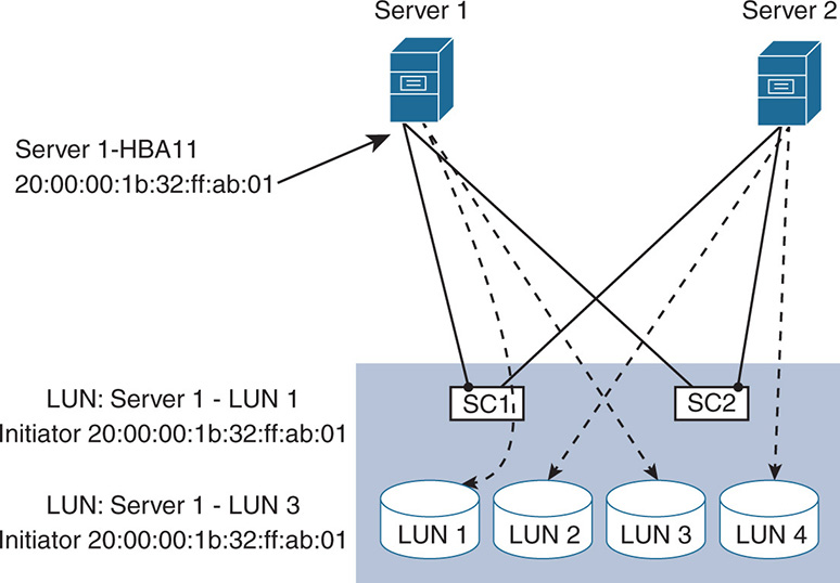
Hosts see all LUNs on a target port. If, however, you wanted a server to see certain LUNs while hiding other LUNs, masking prevents the server from seeing specific LUNs. Masking is done in host software or in the HBAs or, in the case of SAN, on the storage controllers of the storage system. The decision depends on who you trust to make the configuration, because the person configuring the server is different from the person configuring the storage. LUN masking works on the WWN. Figure 2-14 shows how Server 1 has access only to LUNs 1 and 3 on a RAID 5 disk array. The storage controller was configured to allow initiator 20:00:00:1b:32:ff:ab:01 (which is Server 1-HBA11) to communicate to LUNs 1 and 3 and masked LUN 2 and LUN 4 from Server 1. In the same way, the storage controller is configured to allow only the HBAs of Server 2 to initiate connections to LUN 2 and LUN 4.

Figure 2-14 LUN Masking

Fibre Channel Switching

Switching in a fibre channel network is much different from switching in Ethernet and IP networks. The combination of switches and cables is called fabric. Normally, multiple SAN fabrics are configured to ensure redundancy. In FC, each switch is recognized by a unique identifier, called a domain identifier, or domain ID. The domain ID is an 8-bit identifier with values that range from 0 to 255, with some numbers reserved. One of the switches is elected as a principal switch and assigns domain IDs for the rest of the switches.

Start with a Fabric Login process (FLOGI), where the FC switch acts as a LOGIN server to assign fibre channel IDs (FCIDs) to each WWPN. This is similar to IP networks, where a client requests its IP address from a Dynamic Host Configuration Protocol (DHCP) server. The FCID is a 24-bit address that contains the switch domain ID, the switch F_port the FC node is attached to, and the N_port of the end node. The switches maintain a table of WWPN-to-FCID mapping and exchange the tables between switches using the fibre channel network service (FCNS) protocol. As such, each switch has information about every WWPN in the network, including to which switch and switch port it is attached. It uses such information to deliver FC frames. During the FLOGI process, buffer credit information is exchanged between N_port and F_port to be used for flow control because FC is a lossless protocol.

After an FC node finishes the FLOGI process and receives its FCID, it must know the other WWPNs on the network. The initiator node performs a port login (PLOGI) process through a Simple Name Server (SNS) function running in the switch. During the process, each node sends to the switch its mapping between its FCID and its WWPN. The switch collects this information and checks its zones to decide which WWPN (soft zoning) can talk to which other WWPNs. As a result, the nodes receive the WWPNs that reside only in their zones.

After the nodes finish the FLOGI and PLOGI processes, they have visibility into other target WWPNs they can connect to on the network. As such, a host initiator does a process login (PRLI) toward the target storage device it wants to connect to. At that time, the storage controller on the target sends the initiator the LUNs that the host can connect to and masks all other LUNs. This is illustrated in Figure 2-15.

Multipathing

Multipathing provides added redundancy in case of network component failures. Also, multipathing is leveraged for higher performance by having the host use the bandwidth available on multiple paths when reaching the storage. The different paths are formed by using multiple HBAs on the servers, different SAN fabric (switches, cables), and multiple storage controllers with multiple ports. Figure 2-16 shows a fibre channel network where redundancy is added at every level, node, switch, and controller. Notice that there are two different fabrics via switches: SW1 and SW2. The fabrics do not interconnect at the switch level for added security and to limit propagation of misconfigured information between the fabrics. If you remember, in fibre channel switches, one switch propagates the configurations to other switches. Notice that Server 1 is connected to the switches via two different port adapters: S11 and S12. Server 2 is connected to the switches via two port adapters: S21 and S22.

Figure 2-15 Fibre Channel Routing

Figure 2-16 Multipathing in a SAN

S11 connects to switch SW1, and S12 connects to SW2. Similarly, S21 connects to SW1, and S22 connects to SW2. The switches connect to a storage array and are dual-homed to two storage controllers: SC1 (SC11, SC12) and SC2 (SC21, SC22), which in turn have dual ports 1 and 2. With any failure in the network, the system will find an alternate path to reach the target storage LUNs. To limit the number of paths between a host and its LUNs, zoning is applied.

In the diagram, you find four different paths to reach LUN 1 from server 1. The first two paths are via SW1 and are (S11, SW1, SC11) and (S11, SW1, SC21), and the second two paths are via SW2 and are (S12, SW2, SC12) and (S12, SW2, SC22). The controller ports SC11, SC12, SC21, and SC22 form what is called a Target Portal Group (TPG). Information about this portal group is known to Servers 1 and 2, which use this portal group to reach LUN 1 and LUN 2, respectively. Although both storage controllers can reach all LUNs in a disk array, a storage controller can “own” a LUN and is considered the most direct path to that LUN. So, in this case, SC1 owns LUN 1 and SC2 owns LUN 2.

Another protocol used in multipathing is the Asymmetrical Logical Unit Access (ALUA). ALUA allows the storage system to tell the clients which paths are optimized and which are not. In this case, SC1 tells Server 1 that path (S11, SW1, SC11) is optimized to reach LUN 1 because it owns LUN 1. Also, SC1 tells Server 1 that path (S12, SW2, SC12) is another optimized path. The other two paths are nonoptimized because they go through controller SC2.

Given that the hosts have the ALUA information, load balancing is supported through the host multipath (MPIO) software. Traffic destined to a particular LUN in the storage system can actually be sent over two available paths in an active-active mode, thereby doubling the available I/O bandwidth. The decision to choose one path or multiple is left to the OS at the host, which has all different paths to reach a LUN. Server 1 can utilize both S11 and S12 to send traffic to reach LUN 1. In case of a path failure, connectivity remains, but I/O bandwidth is cut in half.

Also note that the storage array itself can participate in the failover. For example, a storage array experiencing a target failure could indicate to the host to reinitiate the connection to connect to the available working ports.

iSCSI SANs

iSCSI provides block-level access to storage devices by carrying the SCSI commands over a TCP/IP network. iSCSI functions are done in software and rely on a traditional Ethernet network interface card (NIC) for connectivity; however, the system performance greatly suffers as the CPU becomes overloaded. A better choice is to use an iSCSI HBA/NIC with a TCP Offload Engine (TOE) function that offloads the CPU from functions such as encapsulation and decapsulation that are better done in hardware. The iSCSI HBA connects to the Gigabit Ethernet network and supports multiple ports and interface speeds such as 1 GE, 10 GE, 40 GE, 25 GE, 50 GE, and 100 GE. Because iSCSI runs over TCP/IP, the packets run on an L2-switched network or IP routed over an L3 network. iSCSI uses IP, so it runs over LANs or WANs. Figure 2-17 shows a typical iSCSI network. Note that both hosts and storage systems connect to a regular Ethernet/IP network. Depending on IT budgets, the storage Ethernet network could be separate from the existing TCP/IP data network; this gives storage transactions the most performance.

Figure 2-17 iSCSI SAN Deployments

iSCSI Addressing

Unlike fibre channel, which works on WWNs, iSCSI addressing is done via the iSCSI qualified name (IQN) or the extended unique identifier (EUI).

The iSCSI IQN can be up to 255 characters and has the following format:

iqn.yyyy-mm.naming-authority:unique name, where:

• yyyy-mm = the year and month the naming authority was established.

• The naming-authority = normally the “reverse” of the authority domain name.

• The unique name = any chosen name, such as a host name.

For example, iqn.2000-01.com.domain.iSCSI:Server1H11 indicates the following:

• yyyy-mm = 2000-01 indicates the year and month the authority “domain” was established.

• Domain name = domain.com, subdomain = iSCSI. So, the reverse is naming-authority = com.domain.iSCSI

• unique name = Server1H11; indicates Server 1, host bus adapter 1 port 1.

The EUI is formed with the prefix eui. and a 16-character name, which includes 24 bits of a company name assigned by the IEEE and a 40-bit unique identifier. An example is eui.1A2B3C4D5E6F7G8H.

Also, like fibre channel, the iSCSI names can be written as aliases for easier representation. For example, an alias of the IQN listed above, iqn.2000-01.com.domain.iSCSI:Server 1H11, could be iSCSI-Server1-H11.

Finally, each iSCSI initiator or target is represented by its own TCP/IP address used to exchange traffic over the IP/Ethernet network. Server1-H11 could be assigned an IP of 10.0.1.1, for example. iSCSI does not support the login processes (LOGI, FLOGI, PRLI), but it does support the concept of a TPG. A set of storage controller IP addresses is grouped in TPG; the initiator must specifically reference its target by pointing to the target IP address within the TPG.

iSCSI Network Segmentation

Similar to FC, where segmentation is done via zones, segmentation in an iSCSI network is done via virtual LANs (VLANs). However, segmentation in VLANs is enforced at the switch level, where the switches pass traffic between ports depending on the port VLAN configuration. This is similar to fibre channel hard zones. Filtering is also done on the MAC addresses; however, because this occurs at the switch level as well, it is a more tedious task to maintain. Also, a level of secure authentication and encryption is accomplished between the initiators and targets to ensure that an authorized initiator accesses a target.

iSCSI LUN Masking

iSCSI LUN masking is supported. As the initiator points to a target via an IP address and a connection process takes place, the target allocates the proper LUNs based on the IQNs and assigns them to a group of initiators. There are many ways of doing LUN masking in iSCSI depending on vendor implementations. Normally this is done on storage controllers, but some implementations put access lists (ACLs) on the initiator side to mask the LUNs. The battle between storage folks and system folks continues, as the storage people want LUN masking on the storage system to prevent unauthorized host access, and system folks want to put the LUN masking on the host just to make sure the storage folks did not misconfigure and expose their data to many hosts. Transitioning into hyperconvergence will hopefully create unified storage/system expertise, where one group is to blame if (or obviously when) a misconfiguration occurs.

iSCSI Multipathing

In an iSCSI environment, multipathing is supported via ALUA and MPIO, as well as by other load-balancing techniques inherited from IP/Ethernet networks. Multipathing is done at the host level using MPIO, with the software having visibility into the different iSCSI ports that connect the host to the network. For example, a host learns through discovery the IP addresses of the targets within a TPG. If the host is connected via redundant iSCSI HBAs, H1 and H2 and the storage arrays are connected via interfaces SC11, SC12, SC21, and so on. Then the host is able to reach such storage via multiple paths, and if one fails, it uses the other. Furthermore, if both host adapters are active, the MPIO software decides to use both adapters for load balancing. Also, because this is an IP/Ethernet network, load balancing and path protection are performed at L2 or L3 through the switches, so traffic is balanced via different methods such as virtual port channels (vPCs), multichassis link aggregation (MLAG), equal cost multipath (ECMP), or other, depending on whether this is an L2 or an L3 network. More on these concepts can be found in Part VI of this book.

Fibre Channel over Ethernet SANs

FCoE works by encapsulating the FC protocol (FCP) over an Ethernet header. Unlike iSCSI, which carries SCSI commands over TCP/IP, FCoE still uses the FCP protocol to carry the SCSI commands, but it extends a traditional FC network over an L2 Ethernet network. Therefore, FCoE is L2 switched but not routed. Unlike TCP/IP, which has many congestion control mechanisms that handle packet loss and flow control, Ethernet on its own needs added functionality in this area. FCoE needed some enhancements to Ethernet to make it lossless. This is done in two standards: Data Center Bridging (DCB) and Converged Enhanced Ethernet (CEE). These two standards define mechanisms such as the Institute of Electrical and Electronics Engineers (IEEE) 802.1Qbb priority flow control to pause the traffic in case of congestion, IEEE 802.1Qau congestion notification to notify the sender of congestion, and IEEE 802.1Qaz enhanced transmission selection for minimum guaranteed bandwidth allocation. Because L2 Ethernet networks do switching at the media access control (MAC) layer while FC does switching based on FCID, mapping must be done between FCID and MAC addresses. The FCoE HBAs now have to deal with both FCP and connecting to an Ethernet network, which is done via NICs. The combined adapter to perform such functions is called a converged network adapter (CNA). The CNA has virtual adapters—one that acts as an Ethernet NIC and the other that acts as an FC HBA. Storage traffic and regular data traffic are separated in different VLANs.

Because FCoE still uses FCP, all that was discussed about FC addressing with WWNN and WWPN still applies. The initiators and targets use the different login protocols, such as FLOGI, PLOGI, and PRLI. And the same FC concepts for zoning and LUN masking still apply.

Although FC remains the most used technology for storage, future data center architectures will move gradually toward Ethernet networks. It is becoming overwhelming and inefficient to maintain two switched networks: Ethernet and FC. Hard-core FC professionals do not appreciate such statements and are comfortable with FC, but the fact is that Ethernet and TCP/IP are more mainstream and better understood than FC. Convergence between the networking layer and the storage layer will happen sooner or later, and technologies like 10 GE, 40 GE, and 100 GE will be at the forefront in enterprise data centers.

Other SAN deployments exist, such as the Advanced Technology Attachment (ATA) over Ethernet (AoE) which is a block-level storage protocol, based on SATA, to exchange commands with disk drives. Like FCoE, the ATA command set is encapsulated directly over an Ethernet frame and switched over an L2 network. Although the ATA command set is exchanged, AoE presents the operating system with the same SCSI commands as FC, iSCSI, and FCoE. AoE is a lightweight protocol that has seen some limited adoption. There are many debates in the industry on the security risks in AoE deployments in shared environments. AoE is open to many attacks, such as unauthenticated disk attacks, denial of service (DoS), replay attacks, and so on.

Kudos to you if you reached the end of this section. Because legacy SAN networks will not disappear overnight, and the storage engineers will not be out of a job soon, it is important that IT administrators have familiarity in all areas to have a better understanding of hyperconvergence.

Storage Efficiency Technologies

Storage controllers in SANs and their roles in creating LUNs and LUN masking were previously discussed. The storage controllers have many other functionalities to improve the fault tolerance and efficiency of the storage system. This functionality is listed because hyperconverged systems must deliver similar and even better functionality to meet the enterprise needs. Some of the main functionality is explored in this section.

Thin Provisioning

Thin provisioning is important in providing an on-demand capacity provisioning. This means that physical storage is purchased when needed and not in advance, thereby minimizing the costs of storage over provisioning. The way this works is by giving the applications the appearance of having enough storage, while in reality a lesser amount of physical storage is available. When the application needs more storage, physical storage is purchased and added to the network.

System administrators tend to overprovision storage for their applications just in case more storage is needed and to avoid storage upgrades and downtimes in operational networks. An application that normally consumes, say, 100 GB in the first year, 200 GB in the second year, 300 GB in the third year, and so on, might get provisioned with 500 GB on day one, leaving a lot of unused capacity that is already paid for. Perhaps you have 10 such servers, so 5 TB of storage is purchased on day one and 20% of it is used the first year, 40% the second year, and so on.

If thin provisioning is used, the application is allocated 500 GB of “thin storage.” This gives the application the appearance of having enough storage, while in reality physical storage is much less at 200 GB. This results in major savings. When applying thin provisioning to storage arrays, the storage array presents LUNs that appear much larger than what the host needs, while actually giving the host just enough physical capacity needed at the time. These LUNs are called “Thin LUNs” in contrast to “Thick LUNs” that are normally provisioned. Furthermore, advanced controllers allow the storage to “reclaim” capacity. If the host releases some of its capacity, the storage controller releases the blocks on the physical disks, hence reclaiming the storage. Figure 2-18 shows thick and thin provisioning of disk arrays.

Figure 2-18 Thick Versus Thin Provisioning

Disk array 1 has six disks at 1 TB each and is thick provisioned as a RAID 0. This means that when presenting the LUNs, you can at a maximum provision 6 TB worth of LUNs, as shown in LUN 0, LUN 1, and LUN 2, each having 2 TB. In this case if, for example, the capacity needed by LUN 0 becomes 3 TB, you are stuck as you run out of disk space, while LUNs 1 and 2 might still have 3 TB left between the two. On the other hand, disk array 2 is thin provisioned as RAID 0. This means that, when presenting the LUNs, you can actually provision, say, 9 TB of total capacity, where LUN 0 gets 3 TB, LUN 1 gets 3 TB, and LUN 2 gets 3 TB. If in this case LUN 0 needs 3 TB or more, you can reallocate the capacity between LUNs and give LUN 0 extra terabytes. It is important to have management tools constantly monitor the storage because the applications think they have enough storage and could use it and will not report a shortage. Constant monitoring must be applied to ensure that the storage used does not exceed the total physical capacity of disks.

Snapshots

Snapshots is a mechanism that allows data to be captured at any given point in time so it can be restored if there is corruption or damage to the data. The system administrator specifies, based on how and how often the snapshots are taken, a recovery point objective (RPO) and a recovery time objective (RTO). RPO represents the maximum data loss that can be tolerated when a failure occurs. RTO represents the maximum time that can be tolerated for a recovery process after failure occurs.

The use of snapshots varies between simple data restoration at a point in time to creation of full backups. This depends on the vendor implementation of snapshots and the level of comfort of system administrators in the vendor’s implementation. The topic of using snapshots for backups is a bit controversial and will be left for a further discussion of primary versus secondary storage. There are many types of snapshots depending on the vendor implementation. Let’s examine just a few to give you a feel for the technology.

Traditional or Physical Snapshots

In this case, when a snapshot is taken, the data is actually duplicated somewhere else in the disk in the same disk array. The duplication is done either within the same volume or in a separate volume. The data creates a separate backup on a different disk array or restores the information if there is an issue with the original volume. The main takeaway is that this type of snapshot consumes disk space because it is an actual mirror copy of the data. For 1 TB of data, you lose 1 TB for every snapshot, and so on. Also, the snapshot takes time to perform because you cannot use the snapshot until the full data is copied into the snapshot volume. During the copy, the original data must be kept as read-only, so the data itself does not change during the snapshot. Figure 2-19 shows how the original volume is physically copied on a snapshot volume. Once data is fully synched, the snapshot is created.

Figure 2-19 Traditional Physical Snapshots

Copy on Write Versus Redirect on Write Logical Snapshots

In contrast with physical snapshots, where actual data blocks are mirrored, logical snapshots are done differently. A logical snapshot is done by copying the index to the blocks (block map) rather than the blocks themselves. The snapshot is mainly a set of pointers to the original blocks. This constitutes major savings in storage capacity and better performance as instant snapshots are created. There are different implementations for logical snapshots, including copy on write (COW) and redirect on write (ROW).

In the COW, when a snapshot is taken, the original block map is copied into a separate snapshot area. Whenever an original block is updated, it is first “copied” to the snapshot area, and then the original block is modified (written). This ensures that if data corruption occurs in the write operation, the original data is restored from the snapshot. Let’s see how this works.

Figure 2-20 shows the original blocks B1, B2, B3 and the original block map that points to these blocks. If there is no data modification, a snapshot (snapshot 1) would just constitute a set of pointers to the original blocks. If, however, after snapshot 1 is taken a write operation occurs on B3, then B3 would be first copied into the snapshot area, and the pointer in the new snapshot (snapshot 2) would be modified to point to the copy. After that, the write operation takes place and the original block B3 becomes B3’.

Figure 2-20 Copy on Write Snapshots

The drawback of COW is that it consumes three I/O operations when a block is modified: read the original block B3, write the block to the snapshot area, and write the modification B3’ to the original area. The more the original data is updated and the more frequent snapshots are taken, the more performance hits are incurred. Also, to get an actual physical snapshot, you need to collect information from all the gathered snapshots. With more snapshots left undeleted, more disk space is consumed.

A more powerful way of taking snapshots is called redirect on write (ROW). Whenever a snapshot is taken, a copy of the original block map is taken, too, and the pointers to the original data are marked as read-only to represent the snapshot. When the original data is modified, the new data is redirected and written to a different area. The original block map is then modified to reflect the new data, while the snapshot still points to the older data. Let’s look at this using an example. Figure 2-21 shows an original volume with blocks B1, B2, and B3. When snapshot 1 is taken, the block map is copied and the pointers of snapshot 1 to B1, B2, and B3 become read-only. When B3 is modified, the modified data B3’ is redirected and written to a new area, and the file system original block map is modified to reflect the new blocks. If a second snapshot 2 is taken, then the snapshot 2 pointers to B1, B2, and the modified block B3’ become read-only, and the file system block map advances upon any new data modification. As such, you minimized the I/O operation from 3 (read, write, write) in copy on write, down to 1 (write) in redirect on write.

Figure 2-21 Redirect on Write Snapshots

The frequency of taking the snapshots could be a lot higher. Snapshots can be taken every few minutes or every few hours or so, and they can be kept for a longer period. Issues might arise with ROW snapshots based on vendor implementations. One issue, for example, is that snapshots can be deleted by simply removing the pointers to the snapshot blocks. This results in many empty blocks scattered randomly on the disk, degrading the performance of I/O operations. To solve this issue, vendors have to do some sort of garbage collection to rearrange the blocks. Another issue with ROW arises from implementations that create a snapshot parent-child relationship. This is called a snapshot chain. In this case, the original data is the parent, and snapshot 1 (the child) points to the parent. Snapshot 1 becomes the parent of snapshot 2, and so on and so forth. So, the block map of any snapshot is linked to the block map of its parent, and that could create performance issues upon reads while traversing the chain. The longer the chain, the more negative the impact on system performance. Implementations can avoid this issue by creating different block maps for every snapshot.

Other variations of snapshots use incremental snapshots, with new ones updating older ones. Other implementations use continuous data protection (CDP), where snapshots are taken whenever there is a data update. Vendor implementations should be careful not to create too much snapshot information at the expense of other factors, such as performance, disk space, and reconciliation of snapshots to restore the original data.

Cloning

In early implementations, cloning was basically used for creating a mirrored copy of different entities, such as a database, virtual machine, storage data, and more. As such, clones consumed storage due to full-copy penalty. In most modern file systems, cloning and snapshots are similar. Clones that are based on ROW snapshots do not incur full-copy penalty. The difference between snapshots and clones is that clones are writable, whereas snapshots are read-only.

As already explained, snapshots are a point-in-time representation of the data and are used for achieving a certain RPO and RTO when restoring data. If, however, the data from the snapshots needs to be modified (writeable), a clone is created from the snapshot, so the delta changes to the data do not affect the snapshots. Clones can be used, for example, to launch the same virtual machine/application over multiple servers. And if you take that clone and put it on different storage systems in different locations, you are actually backing up the data.

Replication

If you think snapshots and cloning are close enough to cause confusion, here comes replication to add more confusion. Replication is the act of making copies to the data for reproducing information or sharing information between systems. For example, database replication in a distributed database system allows users to work on different databases while keeping the information consistent. Some other uses are merging information between two databases to create a large database. Other applications are read replicas to offload a database of heavy operations that are done offline. Imagine that you have a heavily used database that clients are accessing. You want to perform some analytics on the data without affecting the original system. So you do a read replica of the system somewhere else, and you allow information to be read and accessed without affecting the original system read and write operation. Replication is done synchronously or asynchronously. Synchronous means instantaneous and continuous replication, whereas asynchronous is done offline or at time intervals, but not in real time. The difference between cloning and replication is that cloning is done once to create other systems, whereas replication can be continuous and used for synchronizing data in real time. Also, the difference between snapshots and replication is that snapshots are not copies, and they are used for restore. In the context of hyperconvergence, this book discusses how replication addresses host or disk failures as well as achieves disaster recovery (DR) by replicating data between different sites.

Deduplication

Deduplication refers to the technique of removing duplicate data in a data set. Duplication occurs anytime certain files are modified or similar files are sent to multiple people or environments like virtual desktop infrastructure (VDI), where similar information is repeated for every user. If such information is left as is, it not only impacts local storage but impacts backup storage. Deduplication removes the duplicated data, tremendously improves disk space, and minimizes the bandwidth needed for backup storage, especially when done over WAN. Deduplication is performed at the file level, the object level, or the block level. Different vendors justify the pros and cons of each. Now let’s discuss the different types.

File-Level or Object-Level Deduplication

Assume that a 20 MB presentation was sent to five employees and these employees backed up the presentations on their storage system. The storage has 100 MB of the same data lying around. If deduplication is applied, only one file is saved on the main storage system, and 20 MB is consumed rather than 100 MB. This is seen in Figure 2-22.

Figure 2-22 Deduplication at the File Level or Object Level

However, if the five employees update one slide of the presentation and save it again, you end up with five different versions of the same file that all need to be kept. This is one of the drawbacks of deduplication at the file or object level because it does not produce savings whenever different versions of the same file or object exist. Notice in Figure 2-22 that files 1 and 2 are the same, but file 3 has block B4 modified. When deduplication is applied at the file level, one copy of file 1 is kept, and file 2 becomes metadata or pointers that point to file 1. File 3 must remain as is even though most of its data is the same as files 1 and 2.

Deduplication at the Block Level

Deduplication at the block level is much more granular. Deduplication looks at the individual blocks and removes duplicated blocks, keeping only one copy. If a certain block in a file changed, only that block is copied. This is illustrated in Figure 2-23. Notice that you are applying deduplication at the block level for the same files: 1, 2, and 3. The result is that after deduplication, only one copy of B1 to B6 is kept, as well as the modified block B4’. File 3 points to all the unchanged blocks and to newly changed block B4’. As you see, the savings from block-level deduplication are enormous because of the fine granularity.

Deduplication algorithms take a chunk of data and apply hashing on it to find a unique key, which is a bit string. That key identifies whether any other data hashes to the same key. If it does, the data is considered identical and is not saved. If the key does not match, the data is considered different and is saved, but a pointer is kept to point to the data.

Figure 2-23 Deduplication at the Block Level

Various hashing algorithms identify the unique key that describes the data. The Secure Hash Algorithm 1 (SHA-1), for example, produces a 160-bit string hash, and the Message Digest 5 (MD5) algorithm produces a 120-bit hash.

Deduplication at the block level is done with fixed-sized blocks or with variable-sized blocks.

With fixed-sized blocks, hashing is applied on the fixed-sized block and a key is generated. After that, another block of the same size is taken, and so on and so forth. One of the advantages of hashing on fixed-sized blocks is that it reduces CPU processing because the block boundary is known in advance. The disadvantage of fixed-sized blocks is that if the information added or removed causes many blocks to shift, deduplication becomes inefficient. For example, hashing on the blocks of file 1: [paid][-the][-mon][ey--] versus file 2: [I-pa][id-t][he-m][oney], generates a new set of keys for blocks 1, 2, 3, and 4 and saves the data twice, although the information is practically the same. Of course, this is an extreme case. In practical scenarios, when data is modified, inefficiency occurs only on the affected changed blocks that need to be saved.

With variable-sized blocks, the algorithm does hashing on a different sized block, such as 4 KB, 8 KB, or 16 KB, and tries to optimize to find common data. If variable block sizes are used, hashing on the blocks of file 1: [paid-][the-][mone][y---] versus file 2: [I-paid-][the-][mone][y---], you see that only block 1 changed, and blocks 2, 3, and 4 are saved once. The advantage of hashing on variable-sized blocks is better data matching, but the CPU cycles are much higher. As shown next, deduplication is done inline or at the destination. Inline deduplication could become a CPU hog, which reduces the performance of the system and interferes with the processing of the applications. Vendors differentiate in their architectures by minimizing the performance impacts of deduplication.

Target- Versus Source-Based Deduplication

Target-based deduplication is done at the destination storage system after the data is stored. Deduplication at the target usually comes in the form of appliances that perform the deduplication, are integrated with backup tools, or are integrated with the storage array systems. The benefit of target deduplication is that it offloads the host from the added processing and does not require changes to the host software. The drawback of target deduplication is that the target appliance becomes a central bottleneck getting data from all hosts and must have enough processing power to be able to scale.

Source-based deduplication is done at the host, which deduplicates the data before sending it to the target backup system. This is more of a distributed function because each host does its own share of deduplication. This has great benefits in minimizing the bandwidth needed when transferring data, especially over WAN or remote office environments connected via slow WAN links. The drawback of source deduplication is that it affects the performance of the hosts as it competes for processing power with the actual application. It also requires special software on the source in addition to the traditional backup software. Some implementations enhance the deduplication function by offloading this function to hardware adapters on the host. Other implementations minimize the performance hit by performing deduplication after the data is written to cache and acknowledged.

Inline- Versus Post-Process Deduplication

With inline deduplication, the deduplication function occurs in real time as the data is being stored to the target disk. This means that if it is not done correctly, the process of deduplication might interfere with the application performance. Normally, inline deduplication is done at the source host before it is sent to the target storage. Post-process deduplication tries to offload the host from performing the deduplication in real time by storing the data first in a write cache and sending a write acknowledgment to the host operating system so that it continues doing other tasks. After that, the post-process deduplication takes effect. Post-process deduplication occurs when moving the data from the cache to the target storage or after the data is stored in the target storage. This is open to vendor implementation. Semantically, this is how inline and post-process deduplication are defined. However, many vendors deduplicate on writes when they move the data from the cache into the capacity tier, and they still call it inline deduplication.

Local Versus Global Deduplication

Local deduplication is done at the level of an individual storage system. Each system deduplicates the data it receives. Global deduplication is done on a multisystem level, such as multiple hosts talking to each other, or multiple target storage arrays talking to each other. Global deduplication is more costly in terms of processing and more complex. However, with global deduplication, a wider backup and deduplication strategy are achieved because the data visibility is at a cluster of nodes level rather than a single node.

Data Compression

Data compression makes better use of disk space by eliminating redundant information. This sounds like deduplication, but it isn’t. Whereas deduplication works on the whole storage system to eliminate redundant files or similar blocks, compression works at the file level or at the block level to eliminate repeating patterns or unnecessary data. Compression is considered lossy if the compressed file loses information when returned to the original state. An example is the compression of images that results in lower resolution. Lossless compression does not lose information in the compression and decompression processes. Examples of data compression include the elimination of spaces in a file or the elimination and then restoration of a repeating pattern. The compression factors depend on the original file. Some files achieve 2:1 compression; others may achieve more or may achieve less depending on how many of the patterns can be eliminated. A combination of compression and deduplication achieves enormous storage savings. Different compression algorithms exist. An example of a lossless algorithm that has wider acceptance due to its near line speeds when using multicore processors is LZ4.

Disk Encryption

Disk encryption is performed by using self-encrypting drives (SEDs), which automatically encrypt and decrypt the data before it goes to the media. The SED uses a user-provided password called key encryption key (KEK), which allows the encryption and decryption of another key called the media encryption key (MEK). The MEK, in turn, encrypts or decrypts the data to and from the physical media. Storage implementations that use encryption are more costly because SEDs are more expensive than regular HDDs. Disk encryption should not hinder the performance of the system because encryption is done at the hardware level in the disk controller.

Storage Tiering

Storage tiering is the ability to store data on different types of media, including HDD and SSD, depending on parameters such as application performance needs and frequency of data access. For example, some applications that require high performance are better served by having their data stored on SSD drives or SAS drives, whereas lower performance applications do okay if their data is stored on lower speed 5400 rpm SATA drives. Another aspect is whether the data access is hot or cold. Hot data that is accessed more frequently is better served with SSDs, whereas cold data that is not accessed that often is better served with HDDs. The concept of tiering is to divide the storage array in tiers—tier 0, 1, 2, until n—where tier 0 is the fastest with the highest performance and tier n is the slowest. The main driver, of course, is to reduce the cost per I/O and the cost per gigabyte of storage. SSD flash disks are much more expensive than HDDs, and even within HDDs, there are levels of cost performance. Therefore, tiering tries to get the most performance with the least cost. Figure 2-24 shows a storage array that offers three tiers of storage, with SSD flash being the fastest tier, then a SAS HDD tier, and a SATA HDD tier.

The storage array is configured to do automatic tiering, where it monitors the data access for a certain application and decides when and if it needs to move the data from one tier to another. Hot data, as in frequently accessed data, moves to the SSD tier. Warm data, as in accessed but not so frequently, moves to the SAS tier. And cold data, which has not been accessed for a while, moves into the SATA tier. Tiering is also configured to lock an application to a certain tier if the application cannot handle tiering.

Figure 2-24 Tiered Storage Array

The drawback of tiering is that data is being constantly moved between different drives, which introduces added latency that can be avoided by having the data on a single tier. Because tiering architectures introduce fast SSD flash storage, tiering is sometimes confused with caching, which is described next.

Caching Storage Arrays

Caching storage arrays use fast SSDs to temporarily store the data for applications that need high performance and lower I/O access time and for the data that is most frequently used. Although on the surface this sounds like tiering, caching is completely different. In caching, the cache itself is not used as part of the permanent storage, and data is not moved around between fast and slow storage. In caching, the data is copied into cache for faster access, and when finished, it is deleted from the cache, allowing other pieces of data to be copied. So, the cache is not really part of the storage capacity but rather a placeholder for data that needs to be accessed faster. This is seen in Figure 2-25.

Looking back at what was discussed in this chapter, building and scaling storage networks is an art more than a science. There are so many twists and turns that only the experienced storage administrator can handle it, and all of it is shielded from the software virtualization and network engineers. Besides, only those who make a living building fibre channel vouch for its simplicity, while everybody else is in the dark. For the past few years, administrators have realized that designing virtualized networks on top of SANs while meeting the changing demands of applications is not easy. Next-generation data centers will see improvements in the following areas:

• Moving away from centralized storage controllers to a more distributed storage approach that can scale processing

• Designing networks that anticipate failure rather than networks that react to failures

• Moving away from client server–type file systems to a distributed type–file systems

• Better logical volume management where the concept of LUNs becomes obsolete

• Moving away from fibre channel networking altogether because fibre channel switching and protocols are lagging behind the growth curve in Ethernet

• Moving functionality from closed hardware systems into software-defined functionality that leverages x86 processing

Figure 2-25 Caching Storage Arrays

Looking Ahead

This chapter covered most of the basics in storage and storage networking. This is essential in understanding hyperconvergence because most of the discussed principles apply. Hyperconvergence is an evolution of the existing data center designs that still relies on many of the discussed concepts.

However, hyperconvergence is possible because of the evolution of hardware and software that makes host computers faster and storage interconnects faster. And the most important parts are the concepts of software-defined storage (SDS) and software-defined networking (SDN) that form the stepping-stones for hyperconvergence.

Part II of this book discusses the evolution of host hardware and software and how it affects the designs of next-generation data centers. The faster computer processing, coupled with high-speed server-to-storage interconnect and next-generation NICs, makes host computers more powerful than traditional storage arrays. The adoption of software virtualization changed the deployment model and emphasized the application rather than the storage. SDS paves the way for decoupling software from the underlying hardware to allow the move from closed hardware systems to open systems based on x86 processing.