Chapter 17. Application-Centric Infrastructure

This chapter covers the following key topics:

• Cisco Application Centric Infrastructure: A definition of the Cisco application centric infrastructure (ACI) and its purpose.

• ACI Microsegmentation Constructs: Microsegmentation constructs including endpoint groups (EPGs), application network profiles (ANPs), and service graphs.

• Cisco Application Policy Infrastructure Controller: High-level description of the Cisco application policy infrastructure controller (APIC) and its role in pushing the policies, automating, and monitoring the fabric.

• ACI Domains: A description of the different virtual, physical, and external ACI domains and how they are used to integrate policies in virtual and physical environments.

• The ACI Fabric Switching and Routing Constructs: ACI switching and routing constructs, including tenants, virtual routing and forwarding (VRF), and Bridge Domains.

• Virtual and Physical Connectivity to the ACI Fabric: Connectivity into the fabric from both virtual environments such as ACI Virtual Switch (AVS) and physical environments.

• The ACI Switching and Routing Terminology: Description of the different switching and routing terminology such as leaf and spine loopback and anycast Internet Protocol (IP) addresses, mapping database, global and local station tables.

• The ACI Underlay Network: A description of the protocols that run inside the underlay network and the handling of external routes and load balancing inside the fabric.

• The ACI Overlay and VXLAN: A description of the use of VXLAN to normalize the different encapsulations in and out of the fabric; L2 switching and L3 routing are also described in the overlay network.

• Multicast in the Overlay Versus Multicast in the Underlay: Describes how multicast traffic is handled in the overlay and underlay networks.

• ACI Multi-PoD: Describes the use of ACI for automating connectivity and policies between two different data centers while having routing isolation but still under a single APIC controller cluster.

• ACI Multi-Site: The use of ACI for automating connectivity and policies between different sites with different APIC controller clusters but still under a single policy manager.

• ACI Anywhere: How policies and automation can be managed across private and public clouds.

• High-Level Comparison Between ACI and NSX: High-level comparison between ACI and VMware’s networking and security software product (NSX).

Cisco Application-Centric Infrastructure

Application-centric infrastructure (ACI) is a measure to introduce a level of automation into setting and enforcing policies at the application level as well as configuring the switch fabric to support the connectivity requirements of the applications in the data center. ACI uses information related to the applications, such as which tier the applications belong to (web, app, database [DB], or the application environment [development, test, operation, and so on]), to configure the policies appropriately in support of such requirements. Automation of the fabric configuration makes building the fabric plug and play. ACI also aims to have the network offer feedback information such as network health check to understand whether the network is affecting the performance of the application.

ACI puts emphasis on the application for defining policies, regardless of whether the application is virtualized or running on bare-metal servers. This is independent of the physical location of the application and which virtual local area network (VLAN) or Internet Protocol (IP) subnet it belongs to. Applying policies to an application and defining which other application can access it and vice versa is easy on greenfield applications. While setting up the application, you can define polices to define how the application interacts with the rest of the network. However, not all networks are greenfield, and many applications already exist in the network and have a complex interaction with other applications. In this regard, Cisco was a pioneer in the industry in implementing the Cisco Tetration platform, which monitors the packet flows in the network at a fine granularity to identify how an existing application interacts with its environment and how it interconnects with other applications. Cisco Tetration in support of HyperFlex was already discussed in Chapter 11, “HyperFlex Workload Optimization and Efficiency.” Based on Tetration, ACI policies can be intelligently set and monitoring can be done to alarm the end user if there is a deviation from the policy.

ACI focuses on multiple areas such as these:

• Policy setting: This involves automating the configuration of security policies or quality of service (QoS) that are applied on each application. Defining the endpoints for setting these policies is extremely granular. The policies can be set based on a virtual machine (VM), physical or logical ports, names, tags, and more.

• Policy enforcement: ACI enforces the policies inside the fabric at every endpoint. This creates a distributed firewall approach that eliminates centralized firewall overload. For services that need specialized handling, traffic can be redirected to virtual or physical network service appliances for processing.

• Network configuration: This involves automating the configuration of both the overlay and the underlay network. The overlay and underlay were described in Chapter 15, “Software-Defined Networking and Open Source.” This is unique to ACI in the sense that ACI automates both the virtual as well as the physical switching and routing environment.

• Monitoring and feedback: By automating policies and networking for the virtual and physical environments, ACI monitors the network via “atomic counters” and gives feedback on problems that can affect the performance of the application.

ACI is working closely with open source initiatives such as OpenStack and the Contiv project. With OpenStack, ACI integrates with Neutron via application programming interfaces (APIs). In the Contiv project, Cisco ACI is looking to create a uniform environment for implementing microservices in a mixed environment of containers, VMs, and bare-metal servers.

ACI Microsegmentation Constructs

The following is a list of the main ACI microsegmentation constructs in setting and enforcing policies at the application level.

The Endpoint Groups

A base point for ACI is defining the endpoint groups (EPGs). The EPG is a group of applications or components of an application that have a common set of policies. The endpoint could be practically anything you can identify, including a virtual component such as a VM, a docker container, or a physical component such as a server or a network services appliance. The policies are applied to such endpoints regardless of the IP address or the VLAN the endpoint belongs to. An EPG, for example, can be a tier of applications or different components of the same tier. An EPG can represent the web tier (Web-tier), another EPG can represent the application tier (App-tier), and a third EPG can represent the database tier (DB-tier). Different application endpoints are grouped in an EPG, which becomes the instantiation point for the policies and forwarding for the endpoints. An Oracle application, for example, could be tagged as test, development, or production application. Identifying the components of such an application at such granularity and assigning the components to EPGs to apply policy is powerful.

EPGs offer the flexibility to place endpoints into a group based on many attributes—some traditional and some more advanced. For example, at its simplistic level, the endpoints can be defined based on VLANs, IP subnets, L4–L7 ports, or physical ports. However, there is flexibility even at this level, where applications in different VLANs or IP subnets can be in the same EPG undergoing the same policies, or applications within the same VLAN and IP subnets could be in different EPGs undergoing different policies. At a more advanced level, the endpoints can be defined based on VM attributes, an application DNS name, or other.

To further explain with an example, a set of applications is identified via the Transmission Control Protocol (TCP) ports they use. An application such as a web server has access to it and from it identified via TCP port 80. If you group such applications that use port 80 into one group, call that an EPG. When you apply policy to the group, decide whether to allow or deny traffic going to port 80 and that policy is applied to the group. Bear in mind that Web 1 could be on VLAN 100 and IP 20.20.14.0/24, whereas Web 2 could be on VLAN 200 and IP 20.20.15.0/24, which are completely different subnets. This is illustrated in Figure 17-1.

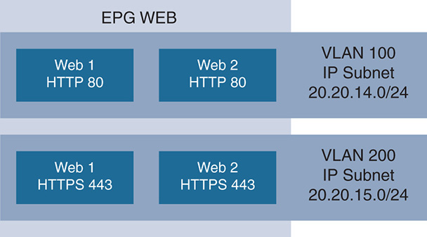
Figure 17-1 Endpoint Groups

Figure 17-1 shows that the EPG contains web applications belonging to different subnets, but all belonging to the same EPG where policy is applied at the EPG level, which could be allowing access to web applications that use the Hypertext Transfer Protocol (HTTP) (TCP port 80) or HTTP Secure (HTTPS) (TCP port 443) services.

Traffic from endpoints is classified and grouped under EPGs based on criteria to be configured. The main methods of classification are based on physical endpoints, virtual endpoints, and external endpoints. External endpoints connect from outside the ACI fabric, such as those behind an L3 wide area network (WAN) router.

The classification of traffic from endpoints and grouping into EPGs depends on the ACI hardware itself and how the connection is made to the endpoint. An ACI fabric could be connected directly to a bare-metal server; be connected to a server running the Cisco AVS switch; be connected to a server running VMware ESXi and the vSphere Distributed Switch (vDS) switch, kernel-based virtual machine (KVM), and Open vSwitch (OVS); be connected to a traditional L2 switch; or be connected to an L3 WAN router. So, the actual classification depends mainly on hardware capabilities and software capabilities of the ACI fabric and what it connects to.

In general, different methods of classification are based on the following:

• VLAN encapsulation.

• Port and VLAN encapsulation.

• Network/mask or IP address for external traffic such as coming in from L3 WAN routers.

• Virtual network interface card (vNIC) assignments to a port group that ACI negotiates with third-party hypervisors such as ESXi, Hyper-V, and KVM.

• Source IP and subnets or media access control (MAC) address, from traffic coming in from a virtual environment like Cisco AVS or from a physical environment like bare-metal servers.

• VM attributes such as the name of a VM, a group naming of VMs, or the guest operating system running on the machine. The classification based on VM attributes depends on whether the information is coming from a host that has software that supports OpFlex (to be described next) such as Cisco AVS or from hosts that do not support OpFlex, such as VMware vDS or other. With AVS, for example, ACI relies on OpFlex to extract the information and does the classification in hardware based on VLAN or VXLAN ID. If, however, the host does not support OpFlex, classification based on VM attributes translates into the MAC addresses of the VMs.

• Based on containerized environments.

Application Network Profile

Now that the endpoints of different applications have been identified and grouped under EPGs and you know how to classify traffic coming into an EPG, you need to define a set of policies between these EPGs. These are called policy “contracts” because they define the interaction between the EPGs based on the set policy. These contracts look like access control lists (ACLs) but are actually very different. Traditional ACLs used to consume lots of entries in the memory of the switches and routers because they are not reusable. Thousands of similar policy entries were written to memory if the source IP, source MAC address, or destination IP or MAC changed. With the ACI contracts, the contract itself is an object that is reusable. Traffic from source endpoints to destination endpoints can reuse the same object contract regardless of IPs and VLANs, which provides much more scalability and consumes much fewer resources in the switch/router memory. The total set of contracts between the EPGs is what is called an application network profile (ANP), as seen in Figure 17-2.

Figure 17-2 Application Network Profile

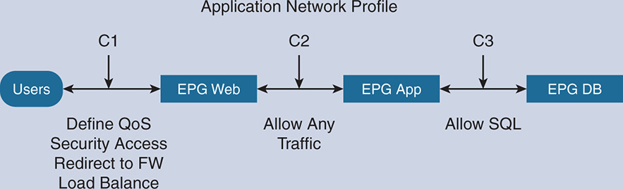
The level of complexity of the policy contract depends on where it is applied. This could be a complex or simple contract. So, Contract 1 (C1) could define quality of service (QoS) parameters, security access parameters, redirection to firewalls and load balancers, or configuration of the actual firewalls. A simple contract such as C2 could be to allow all traffic between the web servers and the app server. C3 could be to allow all Structured Query Language (SQL) traffic from the application server to go to the database server, and vice versa. The policy contract defines both inbound and outbound rules.

The contracts between EPGs have the notion of a consumer and a provider of a contract. This is shown in Figure 17-3. The consumer EPG is the one that initiates the request for a service. For example, when a Web-tier EPG initiates a connection to an App-tier EPG, the Web-tier is the consumer of the contract, and the App-tier is the provider of the contract because it must deliver the service in conformance to the contract.

Figure 17-3 EPG Consumers Versus Providers

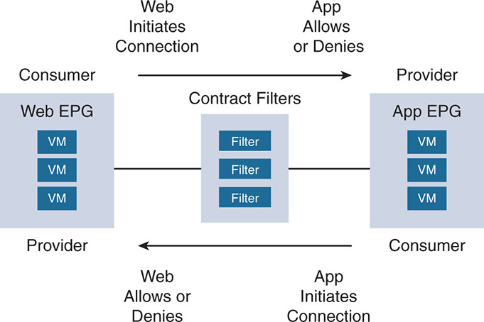
Contracts between consumers and providers are unidirectional. If a Web-tier (consumer) initiates a connection to an App-tier (provider) and the provider allows it, the reverse might not be true. To allow the reverse, the App-tier must become a consumer and the Web-tier must become a provider, and another rule must be defined referencing filters that allow or deny the traffic. In general, connections between endpoints in the same EPG are permitted by default, and connections between endpoints in different EPGs are denied by default unless a contract exists to allow such connections.

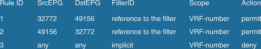
The contract is associated with entries in the content-addressable memory (CAM) that define RuleID, SrcEPG, DstEPG, Scope, FilterID, Action, and more.

A rule references a set of filters and has an action that is applied on the filters. Each of the rules in the CAM is identified by a rule ID, and the rules apply between a source EPG defined by an SrcEPG number and destination EPG defined by a DstEPG number. Also, a contract has a certain scope, where it can be global and used by everyone or belong to a certain administrative domain (tenant) or certain IP forwarding domain virtual routing and forwarding (VRF). The rules that you define are associated with filters, and each filter has a FilterID. Each filter has one or more entries, and these entries are similar to an ACL. The rule has an action. The action taken varies depending on what the consumer requires. For example, an action could allow or deny a certain filter. The action could also mark the traffic to apply QoS, it could redirect the traffic to L4–L7 network services devices like firewalls or next-generation firewalls (NGFWs) or load balancers, it could copy the traffic, log the traffic, and so on. Figure 17-4 is a sample of rules related to a contract as seen inside the memory of an ACI switch. Notice that Rule ID 1 identifies the SrcEPG—in this case, the Web-EPG with a SrcID of 32772 and destination EPG 49156—that is associated with a filter, with the scope being a specific VRF, and the action of the rule to permit the filter. Notice that Rule ID 2 is also needed to define the action in the reverse direction. Rule ID 3 indicates that all other traffic is implicitly denied.

Figure 17-4 Rules Entries of a Contract as Seen in CAM

The filter in this case could classify the traffic based on L2–L4 attributes such as Ethernet type, protocol type, and TCP ports. Figure 17-5 shows a partial screen capture of a filter. Notice that the FilterID is icmp. There is one filter entry called icmp, and there could be more entries in the same filter. The filter identifies the traffic with Ethertype IP. It defines the TCP source port or range and the TCP destination port or range. The rule entry defined in the contract and associated with this filter sets the action on the filter to permit or deny traffic as classified by the filter.

Figure 17-5 Filter Example

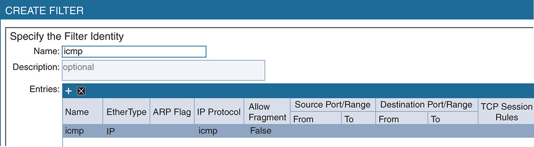
The reason for the hierarchy of having application profiles, contracts, rules, and filters is that Cisco ACI defines everything as objects that can be reused. A filter can be entered once in the CAM and reused by many rules, the rules can be used by many contracts, and the contracts can be used by many application profiles that can in turn be used by many EPGs.

Service Graphs

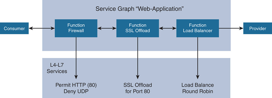
An important policy in the contracts is the service graph. A service graph identifies the set of network or service functions, such as firewall, load balancer, Secure Sockets Layer (SSL) offload, and more, and the sequence of such services as needed by an application. So, for example, say the application is a Web-tier, and the application needs a firewall, SSL offload, and load balancer. Assume that the sequence of actions is such:

Step 1. The firewall needs to permit all HTTP traffic (port 80) and deny User Datagram Protocol (UDP) traffic.

Step 2. SSL offload needs to be applied to all HTTP traffic.

Step 3. Traffic needs to be sent to a load balancer that applies a round robin algorithm to balance the traffic between web servers.

The graph is shown in Figure 17-6.

Figure 17-6 Service Graph

You define a service trajectory with a service graph. Different EPGs can reuse the same service graph, and the service can follow an endpoint if the endpoint moves around in the network. So, if you apply the service graph to a web application inside a Web-EPG and then decide to move the application from one EPG to another, the service profile applies to that endpoint, regardless of whether it lands on a different VLAN or a different subnet. Also, whenever an application is decommissioned, the rules that were pushed into the network service devices are removed from those devices, freeing up resources. If rules are pushed into a firewall, those same rules are removed from the firewall when the application that needs them is terminated.

Cisco has a few ways to allow third-party network services vendors to execute the policies requested by the application and instantiated through a service profile:

• Redirection: The traffic is just redirected to network service appliances. These are either physical devices or software devices. In this mode, ACI does not interfere with what the appliances need to do and just sends them the traffic as was traditionally done in most legacy data centers.

• Device packages: ACI uses the Cisco Application Policy Infrastructure Controller (APIC) to automate the insertion and provisioning of network services rendered by network services devices. To do so, the APIC requires a device package that consists of a device definition and a device script. The device definition describes the device functions, the parameters that are required by the device to configure each function and the interfaces, and network connectivity information for each function. The device script manages the communication between the APIC and the device. The device script is a Python file that defines the APIs between the APIC and the device. It defines the mapping between APIC events and device function calls. The device package is written by third-party vendors and end users, and it is uploaded into the APIC. So, an APIC can map, using the device packages, a set of policies that are defined in a service graph to a set of functions that are implemented by the network devices.

• OpFlex: OpFlex is a Cisco-initiated protocol that allows a controller to talk to a device and give the device instructions to implement a set of functionality. Cisco uses OpFlex as a way for the APIC to talk to the switches and configure the ACI fabric. OpFlex is also being pushed in the standard bodies to have it as an open protocol. OpFlex is different from the Open vSwitch Database (OVSDB) protocol from open source. Unlike OVSDB, which is designed as a management protocol for the configuration of Open vSwitch (OVS) implementations, OpFlex is more of an abstraction layer that does not get into the management or the configuration of the network device. Rather, OpFlex instructs the device to configure certain policies without getting involved in how the device performs the configuration. In the context of ACI, EPGs, and ANPs, OpFlex instructs the network service device like the firewall or the load balancer to implement the contracts between the EPGs. Each network services device must implement OpFlex and map the OpFlex requirements to its own configuration.

ACI Tetration Model

One of the main issues that face IT administrators is knowing the required policies needed for a safe and secure operation of the applications in the data center. Any data center contains newly deployed applications that may or may not interact with existing applications, and existing applications where policies can be enhanced but at the risk of disrupting the existing operation.

As seen so far, the pillars of deploying policies with the ACI fabric are knowing the EPGs and the contracts to be enforced between the EPGs part of an ANP. This is easy to do on newly deployed applications where, at the time of setting the application, the IT administrator knows exactly what the application is, what users need to access it, and what other applications it needs to talk to. Based on that, the IT administrator defines the EPGs and the required interaction.

This might not be so simple if you move into an existing data center that has existing tiers of applications. Some of these applications run on bare-metal servers, others on virtualized environments. A set of policies are already enforced, but whoever set those policies might be long gone and you, the IT administrator, doesn’t even know the exact interaction between the applications. This makes it difficult to identify EPGs, what ports to allow or to deny, and whether applying a new policy to serve a new application could break an existing application. This is where the Cisco Tetration platform plays a big role in giving you insight into the traffic flows and interaction between applications.

Now let’s take a closer look at the Cisco APIC and how it interacts with the rest of the network in the data center.

Cisco Application Policy Infrastructure Controller

The Cisco APIC is the centralized policy manager for ACI and the unified point for automation and management of the ACI fabric. APIC also has open API interfaces to allow integration with third-party L4–L7 network service devices and other platforms such as vCenter from VMware, Hyper-V and System Center Virtual Machine Manager (SCVMM) from Microsoft, OVS, OpenStack, and others. A brief functionality of the APIC controller follows:

• Pushing the security policies into the ACI fabric.

• Automation of the ACI fabric configuration and inventory. Most of the ACI configurations, such as routing protocols and IP addressing, are hidden from the end user. You just need to install the fabric in a leaf spine topology and select an IP subnet to apply for the fabric; the rest of the configuration to allow traffic in and out of the fabric is automatic. The APIC also handles the software image management of the leaf and spine switches.

• Monitoring and troubleshooting for applications and infrastructure to ensure a healthy and operational fabric.

• Fault events and performance management within the logical and physical domains.

• The management of the Cisco Application Virtual Switch (AVS).

• Integration with third-party vendors in the areas of L4–L7 network services, vCenter, vShield, Microsoft SCVMM, OpenStack, Kubernetes, and more.

The APIC connects to the leaf switches in the ACI fabric, and it comes in a cluster fashion, with a minimum of three controllers recommended for redundancy. Each of the APICs connects to a separate leaf switch or has dual connectivity to two leaf switches to protect against a single-point failure. The APIC takes the ANP that was discussed earlier and pushes it to the leaf switches. This is done either as a push model upon ANP configuration or based on endpoint attachments. In the endpoint attachment model, the APIC detects which endpoints (such as VMs in a host) were added and whether they belong to a certain EPG. As such, the APIC pushes the ANP to those endpoints. A policy agent that lives on the leaf switches then takes the ANP policies and translates them into actual configuration on the switches that conform to such policies.

The APIC interacts with the leaf switches via the OpFlex protocol; in turn, the leaf switches interact with the end hosts via OpFlex (in the case of AVS or any endpoint that supports OpFlex). This ensures scalability because you can scale the number of hosts and nodes by scaling the number of leaf switches. The APIC pushes a virtual switch into the server nodes connected to the fabric. The virtual switch could be Cisco’s AVS or VMware’s vSphere distributed switch (vDS). The open source Open vSwitch (OVS) also supports OpFlex, which allows a Cisco APIC to interact with an OVS switch. This is important for implementations that support the open source hypervisor KVM because it adopts OVS as a virtual switch.

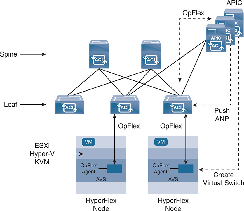
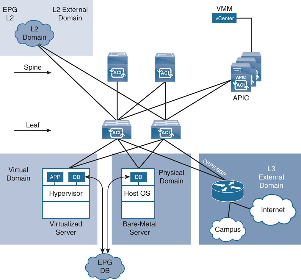
Having a Cisco AVS as a distributed switch has more advantages in the ACI architecture because AVS also acts as a leaf switch and is managed by OpFlex. APIC interacts with the VMs, as well as bare-metal servers, to push the ANPs into the physical or virtual leaf switches (virtual switches) according to the needs of the applications. A high-level view of the APIC interaction with the rest of the network is seen in Figure 17-7. Note how APIC uses OpFlex to interact with the leaf switches. In turn, each leaf talks OpFlex with the virtual environment on the hosts, such as with the Cisco AVS distributed switch.

APIC can create an AVS, a vDS switch, or an OVS. One component of AVS is created inside vCenter and another component is created within a kernel module in the hypervisor. An OpFlex agent is also created in the AVS kernel module, and OpFlex is used to interact with the leaf switches. This is an advantage over creating a virtual switch that does not support OpFlex. In the example in Figure 17-6, the hypervisor is ESXi, Hyper-V, or KVM.

Figure 17-7 APIC Use of OpFlex

ACI Domains

ACI allows the creation of different domains and assigning different entities to these domains to allow the integration of policies for virtualized as well as physical environments. Let’s examine some of the domains that ACI defines.

Virtual Machine Manager Domain

An ACI Virtual Machine Manager (VMM) domain enables you to configure connectivity policies for VM controllers and integrate with different hypervisors. Some of the controllers/hypervisors that ACI integrates with through the APIC are VMware vCenter/ESXi, Microsoft System Center Virtual Machine Manager (SCVMM)/Hyper-V, OVSDB/KVM, and OpenStack. A VMM domain profile groups controllers with similar policy requirements. So, controllers within the same VMM domain can share common elements such as VLAN/VXLAN pools and EPGs. Figure 17-8 is an example of the integration of APIC with a vCenter VMM domain. Because vCenter allows the creation of a data center and puts ESXi hosts inside the data center, ACI allows one VMM domain per data center. So, if vCenter creates a data center east (DC-East) and a data center west (DC-West), you allocate a VMM domain east and a VMM domain west. Each domain shares a separate VLAN/VXLAN pool and separate EPG groups. The following example, as shown in Figure 17-8, is a vCenter VMM domain that interacts with APIC.

Figure 17-8 vCenter VMM Domain

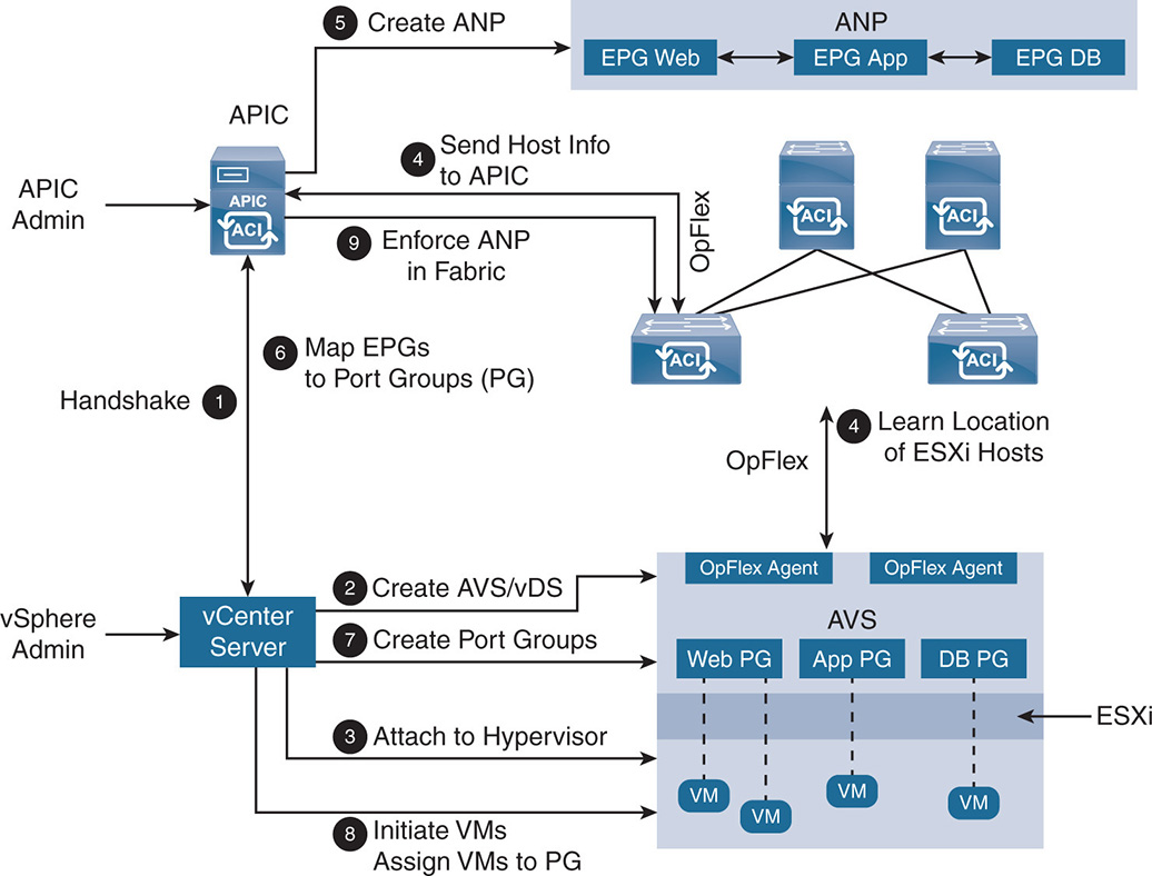
If you take a closer look at how APIC applies the ANP inside the VMM domain, the flow of events proceeds as follows (see Figure 17-8).

Step 1. The APIC performs an original handshake with vCenter.

Step 2. An AVS or vDS virtual switch is created. If AVS is created, an OpFlex agent is created inside the AVS kernel module.

step 3. If an AVS is created, it is attached to the hypervisor. In this example, it is attached to ESXi.

Step 4. All the locations of the ESXi hosts are learned through OpFlex on the leaf switches and are sent to the APIC.

Step 5. The APIC creates the ANP.

Step 6. The APIC maps the EPGs to port groups (PG) that are sent to vCenter.

Step 7. vCenter creates the port groups on the different hosts and allocates a VLAN/VXLAN to each port from a pool of VLANs/VXLANs. As shown in the figure, EPG Web is mapped to port group Web, EPG App is mapped to port group App, and EPG DB is mapped to port group DB. The hosts use the VLANs to allow the port groups to communicate with the leaf switches.

Step 8. vCenter instantiates the VMs and assigns them to the port groups.

Step 9. The policy that is part of the ANP is enforced inside the ACI fabric.

In the previous example, all of the assigned VLAN/VXLANs, EPGs, and ANP profile are associated with the particular VMM domain. This creates separation between the different domains. In addition to vCenter, ACI creates VMM domains for Hyper-V and KVM environments.

Physical and External Domains

Other than the third-party controller VMM domain, ACI allows the creation of physical domains, L2 external VMM domains, and L3 external VMM domains, as shown in Figure 17-9.

Figure 17-9 Integrating Multiple VMM Domains

Physical Domains

A physical domain allows the integration of physical, bare-metal servers with the rest of the virtualized environment. Assume there is an existing database that runs only on a bare-metal server. Now assume that you already created an EPG called EPG-DB that you assigned to a vCenter VMM domain containing database VMs. By assigning the physical server to the same EPG-DB, you can have the bare-metal server as another endpoint in EPG-DB. All of the policies applied to the EPG-DB apply to the physical server. This is done simply by having traffic coming from a specific VLAN on the physical port added to a particular EPG. So, if the physical server is on a specific VLAN and is connected to a leaf switch on a specific port, the traffic coming into that port is put in EPG-DB. Other VLANs on the same physical port are put in EPG-App or EPG-Web accordingly.

External Domains

You can integrate external domains such as L2 or L3 domains with the rest of the ACI fabric, so the newly designed data center based on the ACI fabric integrates with existing L2 networks or campus networks and WAN routers. Such L2/L3 networks form their own domains and have their own EPGs. The whole external network becomes a single EPG by adding all the VLANs in one EPG or is broken into multiple EPGs.

An L3 router forms an external L3 domain peer with leaf switches using traditional L3 protocols such as Open Shortest Path First (OSPF), Enhanced Interior Gateway Routing Protocol (EIGRP), static routing, and internal Border Gateway Protocol (iBGP) [1]. The whole ACI fabric acts as one big switch to the L3 routers. All the protocols running inside the fabric are abstracted from the L3 routers, which see the fabric as one neighbor. This is shown in Figure 17-9, where you see the L3 router peering with the ACI fabric via two leaf switches for added redundancy.

As Cisco tries to simplify the configuration of the L3 protocols running inside the fabric and how information is exchanged, ACI automates the configuration of the fabric so that the end user does not have to know the details. However, it is useful to understand what goes inside the fabric to appreciate the level of complexity. Let’s get into a bit more detail on how the fabric works and how it integrates with the virtual and physical environment.

The ACI Fabric Switching and Routing Constructs

One of the major advantages of the APIC is that it automates the configuration of the fabric. You just add leafs and spines, and the IP address configuration and connectivity are automatically done in the fabric. This is a huge step into the road to hyperconvergence because the whole objective behind hyperconvergence is simplicity and automation. Still, you should not work with a black box; you need visibility into the networking ins and outs if problems occur. The next section gives some details about the ACI fabric, but bear in mind that most of the configuration inside the ACI fabric is automated and hidden from the end user.

Tenant

The ACI fabric is designed for multitenancy, where a tenant acts as an independent management domain or administrative domain. In an enterprise environment, tenants could be Payroll, Engineering, Operations departments, and more. In a service provider environment, a tenant could be a different customer. ACI supports the concept of a common tenant, which is one that has information that is shared with all other tenants.

VRF

ACI defines a virtual routing and forwarding (VRF) domain. A VRF is a private network that is a separate L3 routing and forwarding domain. So, think of tenants as separation at the management level and VRF as separation at the L3 routing and data plane forwarding level. Different VRFs have overlapping IP subnets and addresses and routing and forwarding policies. So, in an enterprise, if you wanted to reuse the IP addresses and separate IP forwarding policies within the Sales tenant, for example, a Local-Sales department could become one VRF and an International-Sales department could become a separate VRF. A VRF that contains DNSs and email servers or L3 WAN routers, or L4–L7 network services devices that must be shared with all other tenants, is normally placed inside a common tenant.

Bridge Domain

Inside a VRF, ACI defines bridge domains (BDs). Think of a BD as an L2 switched network that acts as one broadcast domain and that stretches across multiple switches. Although it’s an L2 domain, the BD could have in it multiple subnets. For readers who are familiar with the concept of private VLANs, think of the BD as a variation of having a private VLAN inside an L2/L3 switch. The primary VLAN is assigned a primary IP subnet and what is called a switch virtual interface (SVI). Beneath the primary subnet, there could be multiple secondary subnets. When routing is enabled on the SVI, it acts as an L3 router between the different secondary subnets. These are the fun tricks in L2 switches that allow them to perform L3 IP switching similar to a router. Private VLANs and SVI were covered in Chapter 1, “Data Networks: Existing Designs.”

The BD is more of a mechanism to control flooding of traffic when traffic is exchanged within the BD. Normally in an L2 domain when a packet arrives with an unknown unicast address or with a broadcast address, it is flooded over all interfaces. In this case the BD controls flooding within itself. A VRF could contain one or multiple BDs.

EPG

Inside a BD, ACI defines the EPGs. The EPG is referenced by an EPG identifier that allows the grouping of many subnets and VLANs within the same EPG. Basically, an EPG is not tied to a physical location, but rather represents a tier of applications. As discussed earlier, all endpoints inside an EPG share a common policy, like a Web-EPG or an App-EPG. A BD has one or multiple EPGs. The insertion of endpoints inside an EPG could be based on physical ports, virtual switch ports, VLAN IDs or VXLAN IDs, tags, subnets, and so on. Also, as explained, the EPGs themselves could be on different IP subnets, so there is a separation between the traditional VLANs and subnets. By default, there is no communication between the EPGs unless the user defines an ANP and defines contracts between the EPGs. Figure 17-10 shows the separation between tenants, VRFs, and BDs inside the ACI fabric.

Figure 17-10 Tenants, VRFs, BDs

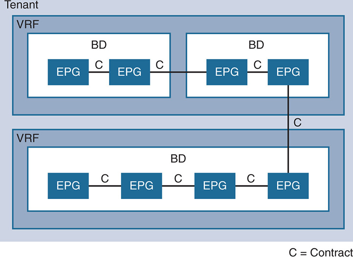
Note how ACI defines private networks or VRFs under the tenant. BDs are inside VRFs, and EPGs are inside bridge domains. ACI also allows information leaking, or route leaking, between the different VRFs, so an EPG inside one VRF could have a contract with another EPG in another VRF.

Virtual and Physical Connectivity to the ACI Fabric

Before looking at networking inside the ACI fabric itself, let’s look at how virtual and physical connectivity are done to the fabric.

Virtual Connectivity to the Fabric

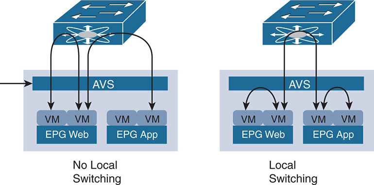
Switching is done between the Cisco AVS and the leaf switches. The AVS itself is a Layer 2 distributed virtual switch that is similar in concept to the VMware vDS. However, AVS integrates via OpFlex with the APICs, allowing better integration between the virtual and physical switches. The AVS works in two different switching modes: Local Switching, and No Local Switching, as seen in Figure 17-11.

• No Local Switching (NS) Mode: In this mode, all traffic from the VMs destined to other VMs in the same EPG or other EPGs that reside in the same physical host is sent to the external leaf switches. This mode is useful if the external switch is analyzing traffic and you need the traffic to be visible to the switch.

• Local Switching (LS) Mode: In this mode, all traffic between VMs in the same EPG in the same physical switch is switched locally. Traffic between EPGs in the same physical switch is sent to the external leaf switches. As shown in Figure 17-11, traffic within EPG-Web is switched inside the AVS, whereas traffic between EPG-Web and EPG-App is sent to the leaf switch.

Figure 17-11 AVS Switching Modes

Cisco does not yet support a full switching mode in which traffic between different EPGs in the same host is switched locally. This is a major area of difference between ACI and VMware NSX (networking and security software product), where ACI relies on the leaf/spine nodes to do the heavy lifting for switching and routing and policy setting, whereas NSX relies on the hypervisor ESXi to do the switching, routing, and policies. It is not straightforward to assume that the ACI way is better than the NSX way or vice versa just based on whether traffic within a physical server should leave the server. Most traffic in a data center is East-West and goes out the physical network interface cards (NICs) and across switches anyway. The main question to ask is whether the whole concept of switching and routing within software will scale to thousands of VMs, hundreds of nodes, and processing at data rates of 100 Gbps.

Physical Connectivity to the Fabric

Connectivity between the user space and the fabric is done directly to the leafs or by connecting existing L2 switches to the leafs. ACI offers such flexibility because it is obvious that not all installations are greenfield, and there should be a migration path between legacy setups and new setups. This section discusses the different alternatives.

When hosts connect directly to leaf nodes, the hosts normally use different (nowadays 10 GE) NICs for added redundancy. Connect the NICs to a pair of leafs for added redundancy.

Figure 17-12 shows a setup in which a host is connected to two leaf switches. To leverage the capacity of both links, the hosts should run what is called a virtual port ­channel (vPC). A vPC allows an end device, switch, or host to have a redundant connection to two other switches while still making the two connections look like one. This allows redundancy of the links and full use of the bandwidth of both links to transmit traffic. Other similar implementations in the industry go by the name multichassis link aggregation group (MLAG).

Figure 17-12 vPC Groups with Leaf Switches

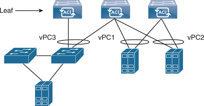
vPC within an ACI fabric does not require the leaf switches to be connected via peer links or peer keepalive links. As a matter of fact, ACI does not allow you to connect leaf to leaf, as the leafs connect to all spines. Different methods can be used to allow the uplinks from the host to share the traffic. Some of these methods are Link Aggregation Control Protocol (LACP) and MAC pinning. LACP allows better use of the uplink bandwidth by distributing flows over the multiple links. MAC pinning involves pinning the MAC addresses of the VMs to one path or the other.

It is worth noting that hosts do not have to be directly connected to leafs because hosts are sometimes already connected to a legacy switching fabric. In that case, the legacy switching fabric itself connects to the leaf nodes.

The ACI Switching and Routing Terminology

Now let’s examine most of the elements needed to understand reachability within the ACI fabric.

• User space: This constitutes all physical or virtual end stations that connect to the fabric.

• Fabric space: This constitutes all elements related to the fabric itself, including the leafs, spines, any physical interfaces on the leafs and spines, any IP addresses inside the fabric, any tunnel endpoints inside the fabric, routing protocols inside the fabric, and so on.

• VTEP: A Virtual Tunnel Endpoint (VTEP) is a network device that terminates a VXLAN tunnel. The network device can be physical or virtual, it maps end devices to VXLAN segments, and it performs encapsulation and de-capsulation. A hardware VTEP could be a physical leaf node or a spine node switch, whereas a software VTEP is the virtual switch inside the hypervisor. In Cisco’s terminology, the IP address of a physical VTEP is called physical TEP (PTEP).

• Leaf node loopback IP addresses: The leaf nodes can have multiple loopback IP addresses as follows:

  • Infrastructure loopback IP address (PTEP): The APIC uses this loopback IP address to address a leaf. Multi-Protocol BGP (MP-BGP) uses PTEP for peering. It is also used for troubleshooting purposes, such as with Ping or Traceroute.

  • Fabric loopback TEP (FTEP): This is a virtual IP address to represent the fabric itself. Consider the fabric as one big switch and the FTEP as the IP address of that switch. The FTEP is used to create an entry point into the fabric from virtual leafs. The virtual leafs are the virtual distributed switches inside a host. The FTEP encapsulates traffic in VXLAN to a vSwitch VTEP if present. The FTEP is also an anycast IP address because the same FTEP IP address exists on all leaf nodes and is used to allow mobility of the downstream VTEPs that exist on the virtual distributed switches inside the hosts.

  • vPC Loopback TEP: This loopback IP address is used when two leaf nodes forward traffic that enters via a vPC. Traffic is forwarded by the leaf using the VXLAN encapsulation. The vPC loopback is shared with the vPC peer.

  • Bridge domain SVI IP address/MAC address: When IP routing is enabled for a bridge domain, the bridge domain is assigned a router IP address, also called a switch virtual interface (SVI). This IP address is also an anycast address that is the same IP across all leafs for the same bridge domain. End stations that are in the bridge domain use this anycast IP address as a default gateway to reach other bridge domains attached to the same leaf or across the ACI fabric. The bridge domain SVI also has a MAC address, and the MAC address is an anycast address in the sense that it is the same MAC address on all leaf switches. So, if an end station moves between one leaf and another, it does not have to change its default gateway because the SVI IP address and MAC address are pervasive and remain the same.

  • Spine-proxy IP or spine-proxy TEP: The spine-proxy IP is a virtual “anycast” IP address assigned to the spine switches. An anycast IP is an IP address that any of the spines use. When a leaf directs the traffic to the spine-proxy IP, the traffic can go to any of the spine switches depending on how the traffic is balanced inside the fabric. Leaf switches use spine-proxy IP or proxy TEP to access the mapping database, where the spine redirects the packets based on the destination MAC or IP address. There are separate spine-proxy TEP IP addresses in the spine. One is used for MAC-address-to-VTEP mappings, one for IPv4, and one for IPv6.

  • Uplink subinterface IP address: A leaf connects to the spines via uplinks. ACI routing inside the fabric is done via L3 protocols such as the Intermediate System to Intermediate System (IS-IS) protocol. ACI does not use routed interfaces inside the fabric but rather routed subinterfaces to exchange IP reachability within the fabric. Subinterfaces give more flexibility in the way a physical interface can be segmented and separated into multiple virtual interfaces that can be used ­differently inside the fabric. ACI uses the subinterfaces to pass the infrastructure VXLAN (iVXLAN) traffic inside the L3 routed fabric.

  • Mapping database: This is a database that exists inside the spine. It contains the mapping of IP host address (IPv4 and IPv6) and MAC address of every physical or virtual node in the user space to the VTEP of the leaf it connects to. It also contains the bridge domains, the VRFs and the EPGs with which they are associated. The spine uses this database to direct traffic such as unicast packets with unknown MAC address or address resolution protocol (ARP) request packets to the leaf (VTEP) that connects to the destination node (represented by the end node destination IP or MAC address). The mapping database is populated using different methods, including processing unknown unicast, ARP broadcast, gratuitous ARP (GARP), and reverse ARP (RARP). It also is populated from information it receives via the Council of Oracle Protocol (COOP) from the leaf switches that gather mapping information from active connections.

  • Global station table (GST): Each leaf maintains a table that maps IP host address (IPv4 and IPv6) and MAC addresses to remote VTEPs, based on active conversations. The GST contains the bridge domains, the VRFs, and the EPGs with which they are associated. This table is a subset of the mapping database that exists on the spine. This way the leaf easily finds which leaf it needs to send the traffic to based on a conversation that took place between two end nodes through this leaf.

  • Local station table (LST): The leaf maintains a table that maps IP host address (IPv4 and IPv6) and MAC addresses to “local” VTEPs, based on active conversations. The GST contains the bridge domains, the VRFs, and the EPGs with which they are associated. This allows fast forwarding between all end nodes connected to the same leaf.

The ACI Underlay Network

ACI uses a two-tier spine/leaf architecture that guarantees there are only two hops between any two end stations connected to the leafs. Layer 3 routing is used inside the fabric to provide reachability between all the fabric VTEPs and to allow the fabric to learn external routes. The fact that L3 is used ensures the ability to do load balancing between the links and eliminates the inefficiencies of L2 mechanisms such as spanning tree.

Different control plane protocols run inside the fabric, including these:

• COOP: Runs on the PTEP loopback IP address to keep consistency of the mapping database. When new nodes are learned locally by the leaf switches, the IP and MAC-to-VTEP mappings are sent to the mapping database via COOP.

• IS-IS: Runs on the uplink subinterfaces between leaf and spine to maintain infrastructure reachability. IS-IS is mainly used to allow reachability between the VTEPs.

• MP-BGP: Runs on the PTEP loopback IP and is used to exchange external routes within the fabric. MP-BGP, via the use of route reflectors, redistributes external routes that are learned by the leafs.

Handling External Routes

The ACI fabric can connect to an external router such as a campus core router, a WAN router, or a Multiprotocol Label Switching (MPLS) VPN cloud. The external router connection is called L3Out and is done via different methods. The first method is done by connecting the external routers to leaf nodes via VRF-Lite and exchanging routes via different routing protocols such as OSPF, EIGRP, iBGP, and static routing. VRF-Lite allows VRF to be built but normally does not scale beyond 400 VRFs. For better scalability, peering with external routers can be done using MP-BGP or Ethernet VPN (EVPN) with VXLAN. This normally scales to more than 1000 VPNs if needed. The external routes are distributed inside the ACI fabric using MP-BGP. Usually a pair of spines are designated as route reflectors (RRs) and redistribute the external routes learned via OSPF/BGP/EIGRP into the leaf nodes. Figure 17-13 shows an example of L3 connectivity to WAN routers via a pair of boarder leafs. The external routes are learned via the leafs and redistributed inside the fabric via MP-BGP. Notice that two spine switches are configured as route reflectors and inject the external routes inside the leafs.

Figure 17-13 Connecting to External L3 Networks

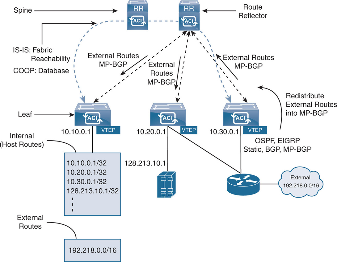
The leafs distinguish internal routes from external routes by the fact that all internal routes in the fabric are host routes, the routes are /32 IPv4 or /128 IPv6 host routes. The terminology /32 indicates a subnet with a 32-bit mask for IPv4 or a 128-bit mask for IPv6, which means the endpoint IP addresses. External IP subnets are recognized by their longest prefix match (LPM). Because the external routes are redistributed via MP-BGP to the leafs, the spines do not see the LPM external routes, but only share host routes with the leafs. The ACI fabric can connect to multiple WAN routers and can pass external routes between WAN routers and as such becomes a “transit” fabric.

ACI Fabric Load Balancing

ACI uses different methods to load balance the traffic between the leafs and the spines. Traditional static hash load balancing can be used. This method does hashing on IP flow 5-tuple (source IP, source port, destination IP, destination port, protocol). The hash allows an even distribution of flows over the multiple links. However, because each flow is dedicated to a path, some flows might consume more of the bandwidth than others. With enough flows passing through the system, you might get close to an even distribution of bandwidth. Load balancing uses the path according to Equal Cost Multi-path (ECMP), where the load is distributed over the paths that have equal cost. In a leaf spine topology, and without adjusting path metrics, all paths between one leaf and every other leaf are equal cost, so all paths are used.

The ACI dynamic load balancing (DLB) measures the congestion levels on each path and adjusts the traffic allocation by placing the flows on the least congested paths. This enhances the load distribution to become very close to even.

The ACI DLB can be based on full IP flows or IP flowlets. When using IP flows, the full flow is assigned to a single path, as already described. However, when using the flowlet option, the same flow can be broken into smaller flowlets, and each flowlet sent on a different path. The flowlets are bursts of packets separated by enough time that allows the packets to arrive at the destination and still in order. If the idle time between the flowlets is higher than the maximum latency of any of the paths, a second burst of packets that belongs to the same flow can be sent on a different path than the first burst and still arrive without packet reordering. The flowlets use a timer with a timeout value. When the timeout value is reached, the second burst of packets is sent on a different path. The aggressive flowlet mode uses a smaller timer, where bursts are sent more frequently, resulting in a fine-grained load distribution, but at the expense of some packet reordering. A conservative flowlet timeout value uses larger timers with less chance of packet reordering, but there is a lesser chance of sending flowlets.

In general, DLB offers better load distribution than static load balancing. And within DLB, aggressive flowlets offer better load distribution than conservative flowlets.

The ACI Overlay and VXLAN

ACI uses VXLAN to carry the overlay network over an L3 routed network. Unlike traditional routing, where the IP address identifies the location of a node, ACI creates an addressing hierarchy by separating the location of an endpoint from its identity. The VTEP IP address indicates the location of the endpoint, whereas the IP address of the end node itself is the identifier. When a VM moves between leaf nodes, all the VM information remains the same, including the IP address. What changes is the VTEP, which is the location of the VM. Note in Figure 17-13, for example, that a VM inside a host is identified with its location (VTEP 10.20.0.1) and its identifier (128.213.10.1).

The Cisco ACI VXLAN implementation deviates from the simple VXLAN use of carrying L2 Ethernet packets over an L3 routed domain. Cisco ACI attempts to normalize the encapsulation inside the fabric by using a different VXLAN header inside the fabric. Cisco uses what is called an infrastructure VXLAN (iVXLAN). For the rest of this chapter, the Cisco iVXLAN is referred to as “VXLAN,” but keep in mind that this VXLAN frame is seen only inside the fabric. Whenever a packet gets in and out of the fabric, it has its own encapsulation coming from physical hosts or virtual instances that could have their own VXLAN headers.

Any ingress encapsulation is mapped into the VXLAN. As shown in Figure 17-14, different encapsulations are accepted on the ingress, including traditional VLAN tagged or untagged Ethernet frames, VLAN tagged or untagged IP frames, other encapsulations such as Network Virtualization using Generic Routing Encapsulation (NVGRE), and the standard IEEE VXLAN encapsulation. Upon receiving the frame, the ACI fabric strips the ingress encapsulation, includes its own VXLAN header, transports the frame over the L3 fabric, and adds the appropriate encapsulation on the egress. The egress encapsulation could be any of the encapsulations that the egress endpoint supports.

The format of an ACI VXLAN packet is seen in Figure 17-15.

Figure 17-14 VXLAN in the ACI Fabric

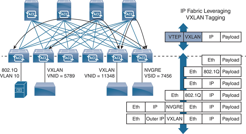
Figure 17-15 ACI VXLAN Packet Format

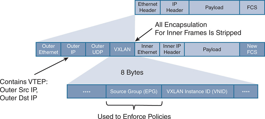
Notice that the VXLAN packet contains a source group identifier that indicates the EPG that the packet belongs to. The source group EPG is used to enforce the policies that are defined in the ANP. The EPGs in the user space map to either VLANs or VXLANs when entering the fabric. As discussed earlier, the leaf node classifies the traffic based on different parameters such as VLAN, VXLAN, IP address, physical port, VM attributes, and more. This classification puts the traffic in a certain EPG, and the EPG is identified in the VXLAN packet via the source group identifier.

Figure 17-16 shows an example of the association between an EPG and leaf nodes based on VLANs and a physical port on the leaf.

Figure 17-16 Association Between EPGs and Bridge Domains

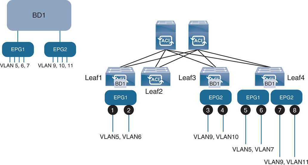
Notice that bridge domain BD1 is spread across leaf switches 1, 3, and 4. BD1 has in it two EPGs: EPG1 and EPG2. The association between EPGs and BD is per Table 17-1.

Table 17-1 BD1 EPG Port/VLAN Mapping

BD1	Leaf 1		Leaf 2		Leaf 3		Leaf 4
	Port	VLAN	Port	VLAN	Port	VLAN	Port	VLAN
EPG1	1	5					5	5
	2	6					6	7
EPG2					3	9	7	9
					4	10	8	11

The VXLAN Instance ID

Inside the ACI VXLAN frame, also notice a VXLAN Instance ID (VNID) that associates the traffic with a certain segment. The VNID allows the proper forwarding of the packet, and it differs whether the packet is L2 switched or L3 routed. In the case of routing, the VNID indicates the VRF that the IP address belongs to, and in the case of L2 switching, the VNID indicates the bridge domain that the MAC address belongs to.

Let’s first look from a high level at an example of a packet that travels into the fabric. Then we’ll go into more detail about L2 switching and L3 routing as shown in Figure 17-17.

As shown in Figure 17-17, a multitude of physical and virtual devices are supported through the fabric. Virtual switches, such as from VMware and Microsoft, can connect to the fabric. The virtual switches have different encapsulations, such as VXLAN for VMware and NVGRE for Microsoft. As such, the ACI fabric “normalizes” the encapsulation by stripping all encapsulation on the input, including its own VXLAN header, and then including the appropriate header on the output. So, if you trace a packet from a VM running on an ESXi hypervisor, it would occur in the following steps:

Step 1. The packet contains an IP header and payload entering the virtual switch or coming from a physical server.

Step 2. With a virtual switch, for example, the switch encapsulates the frame with a VXLAN header and then sends it to the leaf node using the leaf’s VTEP IP address.

Step 3. The leaf node removes the VXLAN header received from the virtual switch and swaps it with the internal fabric VXLAN header. The leaf performs any required policy functions, such as allowing the packet or denying it depending on the set policies. The leaf checks the internal IP address of the frame and verifies its location. In other words, it checks the IP-to-VTEP mapping to locate which leaf it needs to send the packet to. If the egress VTEP is found, it is appended to the frame as the destination VTEP.

If the leaf does not find mapping, it changes the outer destination IP address (the VTEP) to the IP anycast address of the spines. This way all the spines see the frame.

Figure 17-17 Sample Life of a Packet Through the Fabric

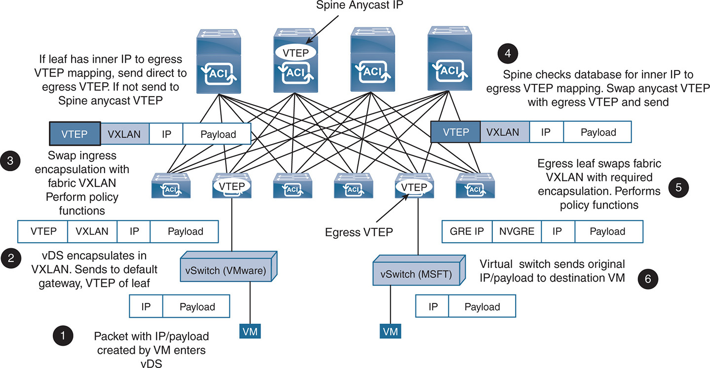
Step 4. The spine that has the mapping changes the egress VTEP to the correct one and forwards the packet to the egress VTEP. All of these steps are done in hardware, with no added latency to the packet.

Step 5. The egress leaf receives the packet. It removes the fabric VXLAN header and encapsulates the packet with the appropriate encapsulation. So, if the packet is going to a Microsoft virtual switch, it is encapsulated with an NVGRE header and sent to the GRE IP address of the virtual switch.

Step 6. Upon receiving the packet, the Microsoft virtual switch strips the NVGRE and sends the IP packet with payload to the destination VM.

L2 Switching in the Overlay

When a source node needs to talk to another destination node, it normally identifies it with its destination IP address. The following are the steps taken when you perform Layer 2 switching in the overlay network. There are generally two cases. The first case is when the destination MAC address in known, and the other is when the destination MAC address is unknown.

If the node that is sending traffic knows the MAC address of the destination, it just sends traffic to that destination MAC address. When a BD receives a packet from an EPG and that packet has a MAC address different from the BD SVI MAC address, the BD knows that this packet is to be L2 switched, not routed, and performs L2 switching. When performing L2 switching, ACI sends the L2 packets over the fabric VXLAN. The L2-switched traffic carries a VNID to identify the bridge domain.

In some cases, the BD receives packets with a destination MAC address that the leaf node does not recognize. This could happen when the leaf node has flushed its ARP table, whereas the server still maintains mapping between an IP address and a MAC address, so the server already knows the destination MAC and does not ARP for it. In normal L2 switching, the switch takes the unknown unicast packet and floods it all over the L2 domain, until the node with that destination MAC address responds. The L2 switch then learns the MAC address through the response packet and includes it in its ARP table so it doesn’t have to perform flooding the next time around.

Because a bridge domain is an L2 broadcast domain, any packet flooding, like ARP flooding or unknown unicast flooding, happens in the whole domain regardless of the VLANs. So, if a packet is flooded in BD1, every EPG and every VLAN associated with the EPG sees that packet. This is done by associating the BD with a VLAN called BD_VLAN, which is a software construct used to send all multidestination packets over the whole BD.

L2 switching is done in two modes: the traditional flood and learn mode and the proxy-spine mode.

In proxy-spine mode, when a leaf node receives an unknown unicast packet, it first checks its cache tables to see if there is a destination MAC-to-VTEP mapping. If there is, the leaf sends the packet to its destination leaf to be switched on that leaf. If the cache tables do not have the destination MAC-to-VTEP mapping, the leaf sends the packet to the proxy-spine, which checks the mapping database. If the destination MAC-VTEP is available, the spine sends the packet to the destination leaf. It is worth noting that the mapping database is always in learning mode for MAC-to-VTEP mapping regardless of whether L2 switching or L3 routing is enabled on the BD. The mapping database looks at active flows coming from the leafs and caches the information or learns the information from the APIC when node attachments take place on the hypervisor virtual switch. Figure 17-18 illustrates the proxy-spine mode.

Figure 17-18 L2 Switching Proxy-Spine Mode

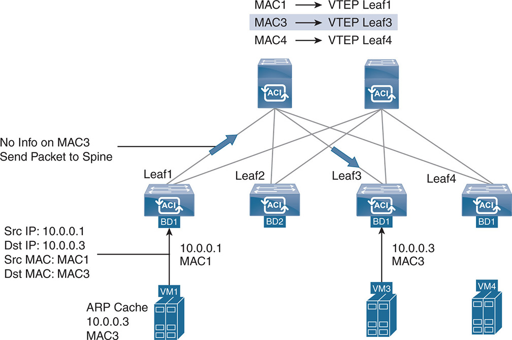
Note that VM1 is sending a packet to VM3, but Leaf1 does not know the MAC destination of VM3; therefore, it sends the packet to the spine. The spine checks its mapping database and finds a MAC-to-VTEP mapping for MAC3 address on Leaf3 and forwards the packet to Leaf3.

Flood mode is not the preferred method of learning MAC destinations, but sometimes it is required. In this mode, ACI floods the unknown multicast packets over VXLAN using a multicast tree. The multicast tree is built using IS-IS, and each leaf advertises the BDs that it has. When flooding is done, the unknown unicast packet goes only to those leafs that contain the particular bridge domain.

ARP handling in the flood mode is similar. When a node needs to send to another node that is in the same subnet, it needs to find the IP-to-MAC mapping for the destination node. This is done by having the source node send an ARP request using a broadcast MAC destination. Nodes that see the broadcast recognize their own IP and respond. Because in an L2-switched mode (routing on the BD is disabled) the mapping is only between MAC addresses and VTEPs, the ARP request must be flooded. The flooding uses the multicast tree similar to the unknown unicast case. This is seen in Figure 17-19.

Figure 17-19 L2 Switching—Unknown Unicast and ARP Flooding in the Bridge Domain

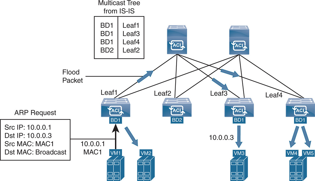
Whenever a packet arrives to Leaf1 from VM1 and the MAC address of the destination is either unknown unicast or ARP broadcast packet, the packet is flooded to all leafs and ports that belong to BD. In this case, the multicast tree that is built using IS-IS indicates that BD1 exists on Leaf1, Leaf3, and Leaf4. Therefore, the packet is flooded to those leafs, and the individual leafs send the packet to all EPGs that are part of that BD. As in regular ARP, once a leaf node learns the local MAC addresses of the nodes that are connected to it, it keeps the MAC-to-VTEP mapping in its local cache table. This prevents further flooding on future packets because the destination MAC-to-VTEP mappings are present in all leafs until they are aged out at some point in time.

L3 Switching/Routing in the Overlay

L3 switching/routing can be enabled or disabled on bridge domains. A bridge domain realizes that a packet needs to be routed when the destination MAC address of the packet matches the bridge domain SVI MAC address. This is like any IP routed environment because the nodes use the router IP default gateway to send packets to subnets that are different from their own IP subnet. The end nodes send traffic to the leaf anycast IP gateway address, which is similar across all leafs for the same tenant. The packet is encapsulated in the fabric VXLAN using the VTEP as the outer source IP and is sent to the destination VTEP IP address to be decapsulated.

In the L3 mode, the inner IP destination (the IP of destination end node) is used to find the IP-to-VTEP mapping. Note that there are two types of routes in the fabric. The routes pointing to IP destinations inside the fabric are represented by /32 host routes or a bridge domain LPM route. External routes are always represented by LPM routes. The leafs first check an IP destination against /32 internal routes and, if not found, the leafs check in the LPM table if the IP destination is within the IP address range of the bridge domain subnets and if found, the leaf tries to find the destination from the spine. If the IP destination is not within the bridge domain subnets, the leaf checks the external LPM routes.

Figure 17-20 shows an example of L3 switching/routing between different subnets across the ACI. Traffic between VM1 10.1.1.1 and VM3 10.3.1.1 is L3 routed. VM1 sends the traffic to the SVI IP gateway, which is the same on all leafs for the same tenant. The MAC address is the MAC of the SVI IP gateway. The leaf checks the inner IP destination of the packet and realizes that it is connected to leaf3 via VTEP 3. The packet is encapsulated in VXLAN with a VNID of 10, which is the identifier of VRF 10, with a source IP as VTEP 1 and a destination as VTEP 3. After the traffic is decapsulated, it is sent to VM3 and IP 10.3.1.1. The IP-to-VTEP mapping as well as VRF information resides in cache tables of the leaf switches.

Figure 17-20 L3 Routing in a Bridge Domain

The VTEP information is exchanged using the IS-IS routing protocol, which is initiated on the subinterface IP address of the uplink between the leaf and the spine. The routing control information is carried across the fabric on what is called an infrastructure VLAN. The L3-switched traffic carries a VNID of 10 to identify the VRF that contains the bridge domains.

In addition to the MAC-to-VTEP mapping, which is always on, the leafs and spines learn the IP-to-VTEP mapping and keep that information in the cache tables and the mapping database.

In L3 routing mode, most of the IP-to-VTEP mappings and MAC-to-VTEP mappings are learned via the source MAC address of the ARP packet or the destination IP address inside the ARP packets. ARP packet handling differs whether ARP flooding is enabled or disabled. If ARP flooding is enabled, the ARP packets are flooded on the multicast tree to all relevant BDs, similar to the ARP flooding in the L2 switching mode. The only difference here is that the leafs and spines populate both their MAC-to-VTEP and IP-to-VTEP mappings because you are in a routed mode.

If ARP flooding is disabled, multiple situations could occur, as illustrated in Figure 17-21.

Figure 17-21 L3 Routing—No ARP Handling

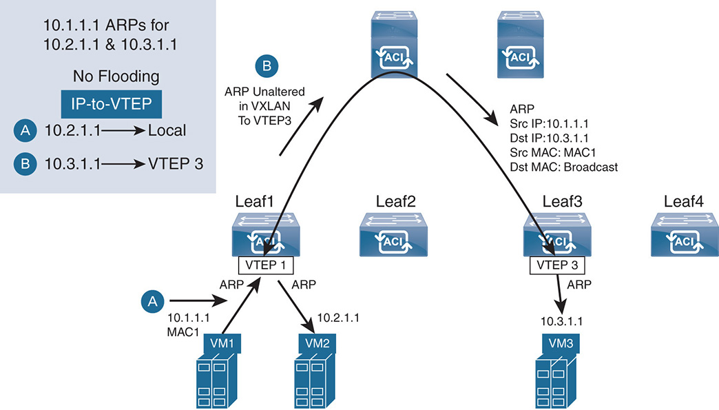
The leaf receives an ARP request, and it knows the IP-to-VTEP destination of the packet. If the destination is local to the leaf, it switches the packet locally to the appropriate local port. If the destination IP-to-VTEP is remote, the leaf sends the ARP unaltered inside VXLAN as a unicast packet destined to the remote leaf. In both cases, if the node is a virtual node on a vSwitch, the ARP is flooded on the appropriate port group on the vSwitch.

If the source leaf receives an ARP request and it does not have an IP-to-VTEP mapping, enter proxy-spine mode. The leaf sends the ARP to the proxy-spine. If the proxy-spine has a mapping, it sends the ARP request unaltered to the destination leaf. If the spine does not have the IP-to-VTEP mapping, it drops the ARP and goes into what is called “APR Gleaning.” In ARP Gleaning, the spine creates its own ARP with a source of the Cisco ACI bridge domain subnet address. The new ARP is sent to all leaf nodes in the bridge domain. In turn, the SVI of each leaf node sends the ARP in the bridge domain. In this case, the bridge domain must have a subnet address.

Multicast in the Overlay Versus Multicast in the Underlay

This is yet another topic that is a bit confusing. You saw how ACI handles flooding inside bridge groups. Multicast is used to allow the fabric to discover which bridge groups belong to which VTEPs. This multicast tree is built using IS-IS, and the multicast addresses that are assigned to bridge groups are called Group IP outer (GIPo), to indicate that this multicast is happening in the underlay network. This type of multicast is called underlay multicast because it is native to the underlay network inside the ACI fabric. Similarly, when using VXLAN between the virtual switches and the leaf nodes, EPGs are segmented using multicast. Each EPG is given a multicast address using an EPG GIPo. When the virtual switch (AVS) sends traffic via VXLAN, it encapsulates the traffic and sends it to the EPG multicast address. The ingress leaf removes the EPG GIPo and inserts the bridge domain GIPo to replicate the traffic to all bridge groups. At the egress leaf, the bridge group GIPo is removed, and the EPG GIPo is inserted to replicate the traffic to all EPGs on the egress side. So far, all of this refers to multicast in the underlay because multicast is native to the ACI fabric.

You also know that the overlay networks are the ones in the user space, or external networks that use the ACI fabric to go from one point to other. In the overlay network itself, there might be a need to run multicast. Hosts, for example, could be running the Internet Group Management Protocol (IGMP), which is a protocol that end nodes and routers use to create a multicast group. If such hosts need to communicate with each other via IGMP, the ACI fabric must find a way to carry such multicast traffic. Such multicast traffic initiated by IGMP is called the overlay multicast. The overlay multicast addresses are referred to as Group IP inner (GIPi) or multicast inside the overlay network.

To carry such traffic, the overlay multicast is carried inside the underlay multicast. Traffic destined for GIPi (overlay) is forwarded in the fabric encapsulated inside the GIPo (underlay) of the bridge domain. Only the leafs that have the particular bridge domain receive the packets using the GIPo address, and those leafs send the traffic to all hosts that are part of the GIPi multicast address.

ACI Multi-PoD

What has been discussed so far applies to a single ACI point of delivery (PoD); you have one leaf/spine network where you run an underlay via IS-IS and MP-BGP, and exchange information between leafs and spines via COOP. Eventually, the single PoD will need to be extended between different locations such as a campus network with two data centers extended over a metropolitan area network. Early implementations of ACI allowed leaf switches called transit leafs to connect between separate locations, creating what is called a stretched fabric. The problem with this approach was that the routing protocols were stretched between clusters creating a single failure domain on the network level.

As such, Cisco added functionality to allow what is called ACI Multi-PoD. With the Multi-PoD architecture, each PoD has its own routing instances, so IS-IS and COOP, for example, do not have to stretch across the data centers, but PoDs still have a single APIC cluster. This is shown in Figure 17-22.

Figure 17-22 ACI Multi-PoD Solution

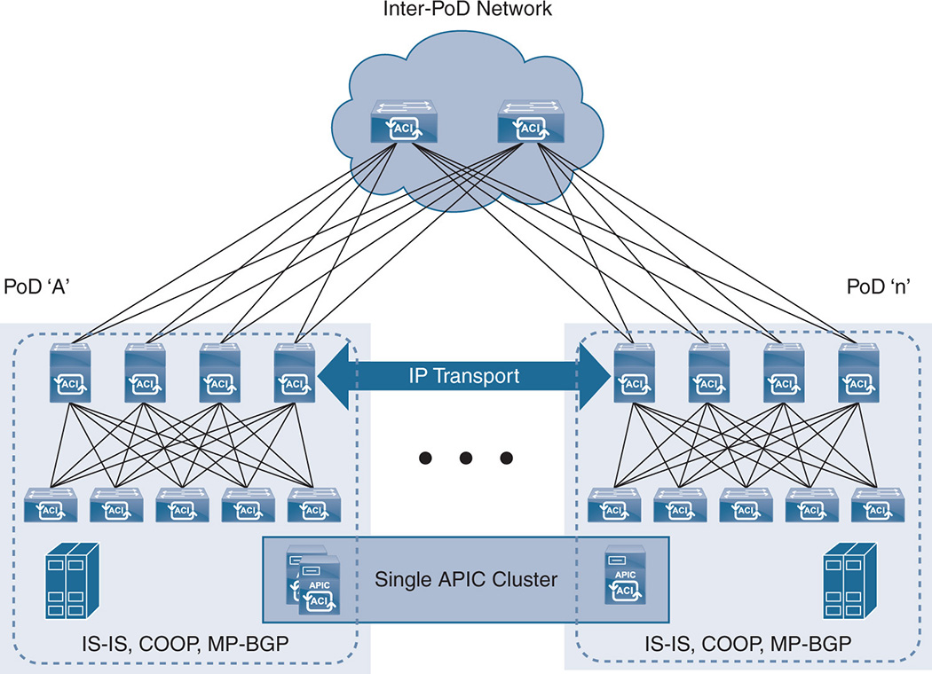
The exchange of information between PODs is done over an L3 IP Network (IPN) but both PoDs are still managed with a single APIC cluster. The two locations act in an active-active mode because, practically, this is still the same fabric running the same APIC cluster controller. Because this is still a single domain, the same policies that the APIC defines are spread across the two sites. The advantage of this design is that it is simple and straightforward; however, the disadvantage is that it represents a single tenant change domain in which policies that are applied at the tenant level are distributed across all sites. So, the concern is about the dissemination of misconfiguration, where a misconfiguration error hits all sites at the same time, which is not good for disaster recovery. In a sense, consider ACI Multi-PoD sites as being part of one availability zone (AZ) because they constitute a single fabric.

ACI Multi-Site

ACI Multi-Site addresses the issue of having a single APIC domain covering multiple sites with a single change tenant with no flexibility to apply policies per data center. ACI Multi-Site solves this issue with the introduction of an ACI Multi-Site Policy Manager. The ACI Multi-Site Policy Manager is a cluster of three VMs that connect to the individual APICs via an out-of-band connection. The VMs are deployed on separate hosts to ensure high availability of the policy manager.

The ACI Multi-Site Policy Manager defines the inter-site policies and pushes these policies down to the individual APICs in each of the data centers, where these policies are rendered on the local fabric. This gives the flexibility of defining similar policies or different policies per data center depending on the requirement. For example, when defining ACI tenants, you can decide to which data center the tenants will stretch and extend the scope of the tenant into multiple sites. ACI Multi-Site creates a separate fabric or separate AZ. This is illustrated in Figure 17-23.

Figure 17-23 ACI Multi-Site

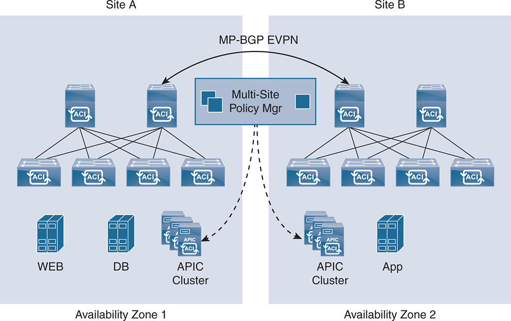
Multi-Protocol BGP (MP-BGP) Ethernet VPN (EVPN) is used to exchange end node reachability, such as IP and MAC addresses. MP-BGP EVPN runs between the spine nodes of the different data centers.

As far as the data plane, L2 and L3 traffic are exchanged via VXLAN across an L3 network that connects the multiple data centers. As discussed earlier, Cisco VXLAN carries segment information inside VNID, such as VRF or BDs depending on whether L2 forwarding or L3 routing is performed. Also, VXLAN carries the source EPG information to exchange the policies. However, because each data center has its own APIC domain, the values of bridge domain, VRF, EPG, and so on, are local to the site. Therefore, a translation function must take place at the spine nodes to translate between the namespace of one data center to the other. This translation function needs enhanced hardware such as the Cisco Nexus EX platform or newer.

ACI Multi-Site can define a schema, which is where you define and manage the ANPs. The schema consists of templates where the actual ANP is defined. For a specific three-tier application, you can define a template whereby you create a VRF and which bridge domains belong to the VRF. Assign the IP gateways and subnets, and define the EPGs that belong to the bridge group. Then define the actual filters and contracts and which EPG talks to which EPG. If the same policies must be applied to a multitier application, the same template can be applied in multiple sites.

In addition to the described functionality, the Policy Manager uses a health dashboard to monitor the health, logs, and faults for inter-site policies.

ACI Multi-PoD and Multi-Site work hand in hand, where Multi-PoD extends an APIC across the same AZ, whereas Multi-Site creates inter-site policies between different AZs.

ACI Anywhere

Other than using ACI Policy Manager to manage policies across multiple private data centers, Cisco uses ACI Anywhere to deliver policy management to private and public data centers. ACI Anywhere allows key attributes of ACI, such as policy management, single pane of glass management, and visibility into the fabric, to be available on public clouds including AWS, Microsoft Azure, and Google Cloud Platform. With Cisco Anywhere, Cisco can, for example, integrate ACI on premise policies with AWS policies such as virtual private cloud (VPC) and security groups. Following are the main functionalities of ACI Anywhere:

• Multi-site management: Gives the users a single pane of glass for managing policies across geographies between multiple data centers for a global view of the policy.

• Integration between private and public clouds: Policies that are used in private clouds can be mapped to public clouds such as AWS. Policies can translate, for example, into AWS VPC and security groups constructs.

• Kubernetes integration: Customers can deploy their workloads as micro-services in containers and define policies through Kubernetes.

• Unified networking constructs for virtual and physical: Unified policies and networking constructs can be defined for virtual environments such as VMs and containers, as well as physical machines such as bare-metal servers.

High-Level Comparison Between ACI and NSX

It is worth doing a high-level comparison between ACI and NSX. Each has its place in the network, and this depends on the use case.

As far as which approach is better, it is hard to make the comparison just based on setting and applying policies. The comparison must be done at a data center level, answering questions about whether you are deploying a VMware cluster that starts and ends with VMware or whether you are deploying a fabric architecture that supports virtual and physical environments. Such environments consolidate legacy and new data centers and multivendor solutions including Hyper-V and KVM. Also, when you discuss the data plane and packet forwarding, the difference becomes obvious between software-only solutions and hybrid software/hardware solutions.

Both ACI and NSX address policy setting and the L2/L3 networking. This is essential for simplifying the deployment of security and networking in hyperconverged environments. Implementations that do not address such automation fall short in fulfilling the promises of simplicity in deploying hyperconverged data centers.

From a high level, both ACI and NSX look similar. They both address the automation in setting policies and simplifying the configuration of the network. A virtualization engineer who is familiar with VMware will probably use NSX for setting policies, while a networking engineer would be more familiar with using ACI. From a commercial point of view, nothing comes for free. The investment with NSX is in NSX licenses, whereas the investment with ACI is in hardware that supports ACI and the APIC appliance with an optional Tetration appliance. So, the decision of which to choose goes beyond policy settings. Make your decision based on the following:

• Policy setting

• Policy enforcement

• Performance requirements for VXLAN

• Stability of the control plane

• Performance of the data plane

• Automation and visibility in the fabric

• Networking learning curve

Policy Setting

For policy setting, the NSX starting point is the hypervisor with closer visibility to the VMs and the ability to perform networking services at the vNIC level. The starting point for Cisco ACI is the fabric. Instead of applying policies inside the host, ACI uses different ways to classify the traffic coming from the VMs into EPGs, and it applies policies at the EPG level.

The main difference between the two approaches is that ACI is a superset of NSX. The flexibility of setting the endpoints in the fabric allows the endpoints to be virtual or physical. It allows the user to break out from the vCenter construct where everything revolves around VMs. An EPG can have physical endpoints such as bare-metal servers, virtual endpoints such as VMs and containers, and physical or virtual network service appliances. In an NSX environment, everything is done at the virtual endpoint level only. Also, because the ACI VXLAN carries the srcEPG information, policy setting is achieved on a single site or multi-site basis for both virtual and physical.

Policy Enforcement

As far as implementing the policies, NSX and ACI have major differences. NSX does the enforcement in software at the vNIC level with the use of the distributed firewall (DFW), whereas ACI does the enforcement at every leaf switch level and in hardware. Anyone who has been in the networking industry for a while knows that the original firewalls were done in software in routers but slowly moved into hardware, either in adjunct cards or external appliances. So, you cannot ignore that software solutions will challenge the central processing units (CPUs). One might argue that because you are distributing the policy enforcement over multiple hosts rather than centralizing it, the performance impact is minimal because the load on each host is smaller. This might be true, but if you start loading the hosts with hundreds of VMs and eventually containers, connect NVMe drives, and pump up I/O to millions of input/output operations per second (IOPS) and the networking connectivity to 40 GE and 100 GE, you will need hardware assist at the host level. So, deciding whether policy enforcement is done in the host or the switch really depends on whether you believe that the host can scale in performance to handle current and future performance needs. Comparing an NSX DFW to ACI’s policy enforcement is like comparing a software-based L4–L7 firewall with a hardware-based L4–L7. Both firewalls are distributed because even with ACI, the firewall function is distributed between all the leaf nodes.

Notice that the DFW and ACI were referred to as L4–L7, not next-generation firewalls (NGFWs). This is because DFW and ACI do not do policy enforcement at the application level. Such functionality is still suited for hardware-based NGFW application firewalls that get inside a session and do filtering based on application constructs. The issue of having NSX working only on the VM level is that NSX enforces policies and redirects traffic within the virtual environment. Although VM-based NGFWs and hardware-based NGFWs offer similar functionality, VM-based NGFWs have a fraction of the performance of the hardware version.

For NSX to tap into the physical environment, NSX must use centralized L2 software gateways such as the Edge Services Gateway (ESG) or centralized third-party hardware gateways. These gateways must stitch the VXLANs inside NSX with VLANs in the physical environment on a one-to-one basis. Added control mechanisms such as OVSDB must be used between NSX and third-party hardware gateway vendors to relay information between the virtual world and the physical world. So, getting the virtual and physical environments integrated in an NSX world is a bit complicated and might cause performance issues due to centralization. In an ACI environment and with classification at the leaf switch level, integration between physical and virtual is more built in.

Performance Requirement for VXLAN

In NSX, the VXLAN processing is done in the hypervisor. In ACI, the VXLAN processing is done in the switch. It is well recognized that VXLAN encapsulation and decapsulation—doing checksum for received packets, packet queuing, packet segmentation, and so on—are better with hardware assist. Even VMware recognizes that fact [2] and recommends using NICs that support VXLAN offload functions. Some examples of offload include TCP segmentation offload (TSO), which allows ESXi to send large packets to the NIC, and then the NIC splits the packets into smaller MTU size frames to be sent on the physical wire. Because VXLAN is a UDP packet, some NICs do not support it, which adds major overhead on the CPU. Other examples are in receive-side checksum offload where, if the receive-side NIC cannot do the checksum, it must be done by the CPU with big overhead. Other areas of NIC performance enhancements are in NetQueue and Receive Side Scaling (RSS), which distributes traffic based on MAC addresses or flows based on hashing. Such techniques bring major performance enhancements in dealing with VMs having to access the NIC and how the traffic is equally distributed between queues and processed in a parallel fashion inside the kernel.

Having VXLAN inside the host rather than the leaf switch can bring major overhead on the CPU if it is not dealt with in hardware. Advanced leaf switches with ASIC technology on the line cards can improve performance in this area. In this particular area, using NSX or ACI depends on how you envision accelerating the VXLAN-related processing at the host level or at the switch level.

Control Plane

Another area of difference between NSX and ACI is where the networking control plane lives. In ACI, the control plane still runs on the fabric. The leafs and spines run protocols like IS-IS, OSPF, EIGRP, and MP-BGP. Although an APIC automates the policies and configuration, the brain of the control is still within the fabric. In the NSX model, the control plane is spread out between the distributed logical router (DLR) VM modules, the NSX controllers, and the ESG. This is perfectly fine because control planes run in CPUs anyway, whether the CPU is on a switch or inside a host. As long as there is enough CPU power not to choke the control, the control plane runs fine. The issues that might arise must deal with the stability of the system itself. With hyperconvergence, you move from an environment where physical servers did the compute while fiber channel switches and storage arrays handled the storage to an environment where the host is running tens of VMs and supporting a distributed storage system with terabits of attached storage. Because hyperconvergence also adds networking to the mix, you have to step back and wonder whether networking is best suited inside the host or in the network fabric where it always was.

A node failure in a hyperconverged vSAN cluster now results in a possible failure of the DLR controller VM, which means another DLR controller VM must take its place. The active peering between the failed DLR and the NSX edge has to be established. The failed node also could have been running the Unicast Tunnel End Point (UTEP) that is carrying the multicast to other nodes.

The bottom line is that a failed host can affect the routing control plane, and the system must stabilize. Depending on the software implementation, the transition period until the system stabilizes and converges will affect networking and storage. So, trusting in one implementation versus another has to deal with your confidence in the stability of the networking control plane in hosts and how fast it converges because it took quite a while for switch vendors to reach the level of maturity you tend to take for granted now.

Performance of Data Forwarding

Another area to consider is the pros and cons of having data forwarding inside the kernel versus data forwarding in leaf and spine nodes. Let’s divide this into two parts:

• Switching within a host: When switching or routing data within a host, NSX uses the vDS inside the kernel to switch and route the traffic. Cisco ACI can choose to do L2 switching inside the Cisco AVS or send the traffic to the physical leaf switch. One might argue that switching inside the kernel introduces less latency because you do not have to go to the NIC card, then to the switch, and back to the kernel. This is true if enough vCPUs are allocated to the switching function, which includes parsing of multiple headers inside the packet. However, if you need to do traffic monitoring and analysis, you are better off sending the traffic to the leaf switch, where traffic analysis is done in fast hardware ASICs.

• Switching between hosts: Most of the East-West traffic between the Web-tier, App-tier, and DB-tier is normally exchanged between VMs that exist in different physical servers. This is done to ensure high availability so you do not lose multiple tiers in the event of hardware failure. In a way, most of the traffic in the data center must travel across the VXLAN tunnels and the fabric from one physical host to another physical host. This is where hardware assist makes a difference because traffic must be encapsulated and decapsulated in VXLANs tunnels, and the host must deal with packet parsing, checksums, security enforcement, and more. As NICs move to 40 Gbps and 100 Gbps and you deploy Peripheral Component Interconnect express (PCIe) buses with NVMe, the CPUs fall short on performance. Hosts need to use Smart NICs that practically offload most of the tasks from the CPU.

On the other hand, in an ACI model, all data forwarding functionality, such as VXLAN encapsulation and decapsulation, switching between VXLAN tunnels, fine-grained policy enforcement, and switching and routing at 40 Gbps or 100 Gbps per port, are offloaded to the leaf switches. These switches exist today and keep getting commoditized and dropping in prices. Having next-generation NICs capable of offloading the CPUs for a wide range of advanced functionality is still under development and might turn out to be costly.

Automation and Visibility in the Fabric

In both ACI and NSX models, everyone agrees that there must be a fabric, and the fabric needs to move from the traditional three-tier access, distribution core to a leaf and spine design. So, the decision here is not whether to use NSX or ACI. The question is how intelligent you want your fabric to be. The Cisco ACI fabric brings a level of automation, where you just add leafs and spines and the system configures itself. ACI also brings a level of visibility in both the virtual space and the physical space. By using telemetry and atomic counters for checking on the health of the fabric, the end user can easily pinpoint whether any performance issues in an application are caused by the network.

One can argue whether this level of sophistication in the fabric is needed or not. The whole mantra of hyperconvergence is simplicity and getting to a level where clusters of compute, storage, and networking are built in minutes rather than weeks. For achieving such goals, introducing fabric automation via ACI becomes a must.

Networking Learning Curve

For environments that are 100% virtualized and VMware heavy, VMware virtualization engineers are probably more comfortable with NSX. It is unlikely that virtualization engineers will handle NSX routing because networking engineers who are involved in building the underlay network will have to get involved for the overlay. Networking engineers will have to go through a learning curve adopting the NSX switching and routing model that is still in the infancy stages. Networking engineers might still decide to go the ACI route for networking and network automation, leaving the policy setting and enforcement to the virtualization engineers.

On the flip side, if the fabric requires a mix of virtualized and physical environments, then networking engineers will have the task of building an ACI overlay and underlay. For setting policies, choosing NSX is more challenging in combining virtualized and physical environments. Cisco is facilitating the jobs of network engineers with the Cisco Tetration to become more familiar with the policy requirements of the applications. This will help the network engineer take control of the policy setting and enforcement within the ACI framework.

To conclude, in a VMware virtualized environment, virtualization engineers might find it more straightforward to play with policies. However, when it comes to switching and routing and integration between virtual and physical, NSX is challenging to networking engineers. A networking engineer who is used to advanced functionality in switches and routers and specifically with ACI will be constrained with what NSX does and will have to go through a steep learning curve.

ACI, on the other hand, is challenging to virtualization engineers and will probably need a networking engineer to launch it. Cisco is doing its best to enhance fabric automation and to bring application visibility to networking, to the point where all networking engineers will be very familiar with virtualization.

As far as investments, it is unrealistic to assume that with NSX, the user would not have to invest in advanced fabric functionality. With or without ACI, network switches will continue to evolve and enhance functionality to offer higher speed interfaces and hardware assist for specialized services such as firewalls, encryption, telemetry, encapsulation, and indexing. So, whether you like it or not, the fabric is evolving, and investment in newer and advanced switches must be done.

Looking Ahead

Part VI covered the networking aspect of hyperconvergence. Automation in networking is essential to the plug-and-play aspect of HCI.

One area of importance that wasn’t covered yet is the concept of hybrid clouds and multicloud. As the adoption of cloud services skyrockets, it is important to understand how HCI fits in the multicloud model.

Part VII of this book discusses cloud services in general, with a special focus on Amazon Web Services (AWS). It then discusses how HCI integrates with one or more clouds and how vendors are helping users find the right cloud model to run their applications.

References

[1] Internet Routing Architectures. Sam Halabi. ISBN-13: 978-1578702336, ISBN-10: 157870233X.

[2] https://www.vmware.com/content/dam/digitalmarketing/vmware/en/pdf/whitepaper/vmware-vsphere-pnics-performance-white-paper.pdf