Chapter 3. Texture Creation

In the beginning, somewhere back in the 1980s, a rotating 3D cube was an amazing thing to see. Today, the realism of 3D animation can be very eye-catching, but a good part of this realism comes from two key factors: lighting and surfacing. Gone are the days of rendering objects with simple colors. Today you need to add images, textures, grunge, dirt, shine, reflection, and more to your 3D models to make them look the best they can. In your 3D career, professional or otherwise, you’ll find that achieving this realism is a never-ending battle. Note, however, that this struggle is a blessing in disguise. Your mission, should you choose to accept it, is to continually better your work. Once you create a fantastic piece of 3D art, it’s time to make a better one! Without forgetting that lighting setups play a big role in determining the realism of your scenes (we’ll get to that in Chapter 4), this chapter will introduce you to LightWave’s texturing capabilities. This chapter helps you take the next step with LightWave by introducing you to the powerful Texture Editor and teaching you how to navigate and use its interface. You’ll learn about these topics:

• Using the Surface Editor

• Organizing surfaces

• Setting up surfaces

• Understanding the Node Editor

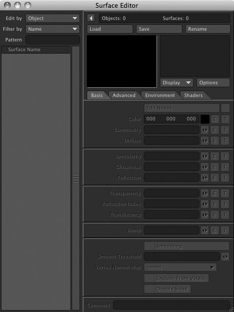
Perhaps one of the best things about LightWave’s Surface Editor is that it puts everything you need to set up simple-to-complex surfaces in one location. The Surface Editor gives you control over everything you need to create a blue ball, an old man, or a modern city. If you’re familiar with the Surface Editor in previous versions of LightWave, you’ll find the updated Surface Editor works in much the same way but is definitely improved. Most notably, LightWave v10 brings excellent texturing to the table with both the Surface Editor and the Node Editor. Figure 3.1 shows the Surface Editor interface at startup, with the Node Editor open.

Figure 3.1. LightWave’s Surface Editor at startup.

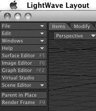
You’ll get a brief introduction to the Node Editor in this chapter. It’s important to understand how basic texturing works, and the Surface Editor is the place to start. In early versions of LightWave, the process of setting up a model’s surfaces began during construction, in Modeler. However, you could make only basic surface changes in Modeler—essentially, you could select a group of polygons and name them as a surface. Defining and applying surface attributes such as color and shininess, or adding more complex textures, required moving over to Layout. In LightWave v10, the Surface Editor is accessible in both Modeler and Layout, so you can set up surfaces in either part of the program. This chapter applies to both Modeler and Layout, except for the section on the Node Editor, which is available only within Layout. And while you can access and apply node-based surfacing in Modeler, you can’t render, so you won’t have much of an idea of what your surface will look like. The Surface Editor button is sixth from the top in Modeler (Figure 3.2) and fifth from the top in Layout (Figure 3.3). The F5 key also opens the Surface Editor in both Modeler and Layout.

Figure 3.2. LightWave’s Surface Editor can always be accessed at the top left in Modeler.

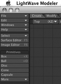
Figure 3.3. LightWave’s Surface Editor is the same in Layout, and it’s always accessed at the top left of the interface.

Using the Surface Editor

As mentioned earlier, all of your surfacing needs can be accomplished within the Surface Editor, so you should be familiar with its features. This section guides you through its uses and helps you make sense of the panel. It’s much easier than you might think! As with any task, you start by getting organized.

Organizing Surfaces

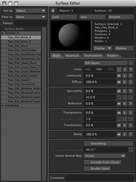
Good management of your 3D work, from models to keyframes to surfaces, will help you become a better artist. The Surface Editor makes it easy for you to manage your surfaces. Figure 3.4 shows the Surface Editor as it appears when an object with multiple surfaces is loaded into Layout.

Figure 3.4. The Surface Editor enables you to manage your surfaces easily on an object or scene basis. You also can use filters to organize your surfaces by name.

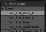
When you open the Surface Editor after a scene has been loaded, the scene’s surfaces are listed in the Surface Name list, as you can see in Figure 3.4. The Surface Name list contains information on every surface in the scene; by default it groups surfaces by object. Clicking the small triangle next to an object’s name reveals a list of all the surfaces associated with that object. Note that by default, if an object is selected in Layout when you open the Surface Editor, its first surface will be opened in the Surface Editor. Figure 3.5 shows the same scene as Figure 3.4, but with a surface of the first object selected. Note that this setup is using the Edit By Object selection from the top left of the Surface Editor, which lists the surfaces with their appropriate objects.

Figure 3.5. Surfaces are grouped with their respective objects if Edit By Object is selected.

When you click the small white triangle next to a surface name in the surface list, your surface settings, such as color, diffusion, or texture maps, won’t be available until you click a surface name. You must select one of the surfaces in the list before you can begin to work with it. When you select a surface, you see the surface properties change. Working with a hierarchy like this is extremely productive and enables you to quickly access any surface in your scene.

To save screen space, LightWave’s Surface Editor allows you to collapse the Surface Name list by clicking the button marked with a right-pointing triangle above the Load button at the top of the panel. Figure 3.6 shows the Surface Editor with the collapsed Surface Name list. Click the button again (it now points left) to expand the list, or choose a surface using the Scene drop-down under Surface Name at the top of the panel, as in Figure 3.7.

Figure 3.6. You click the small triangle at the top of the Surface Editor panel to collapse the Surface Name list.

Figure 3.7. You select surface names in a collapsed view by using the Scene drop-down list under Surface Name.

Selecting Existing Surfaces

Take control of your surfaces, and you’ll have a better time navigating through the Surface Editor panel. You have three modes to assist you in quickly selecting the surface or surfaces you want:

• Edit By

• Filter By

• Pattern

The Edit By drop-down, found at the top-left corner of the Surface Editor panel, has two options: Object and Scene. Here, you tell the Surface Editor to control your surfaces within just that, an object or the scene. For example, let’s say you have 20 buildings in a fantastic-looking skyscraper scene, and eight of those buildings have the same surface on their faces. Using Edit By Object, adjusting that surface’s characteristics would mean applying surface settings eight times; with Edit By Scene, changes to surface settings apply globally to all objects that contain that surface.

You should always be aware of the Edit By mode when you’re tweaking surfaces. (LightWave remembers the Edit By setting when it saves models and scenes, so check each time you start the program to make sure you’re in the mode you think you’re in.) Applying and saving scene-wide changes when you mean to change only one object can have grim consequences. To avoid this, always make each surface name unique, and name your surfaces accordingly when building objects. For example, let’s say you created a slick interior for an architectural render. In it, there are lots of white marble surfaces. (Why? Who knows, but that’s what the client wanted.) To properly isolate and organize those surfaces, you should name the different surfaces so they are unique to the geometry but familiar to you. You could choose something like “interior_marble_stairs,” then “interior_marble_columns,” and so on. This way, there is no confusion when using the Surface Editor. In addition, creating and naming surfaces properly in Modeler makes surfacing easier, and you end up using the Edit By feature as an organizational tool, not as a search engine.

At the top-left corner of the Surface Editor panel, you’ll see a Filter By listing. Here, you can choose to sort your surface list by Name, Texture, Shader, or Preview. Most often, you’ll select your surfaces by using the Name filter. However, say you have 100 surfaces, and out of those 100, only two have texture maps. Instead of sifting through a long list of surfaces, you can quickly select Filter By and choose Texture from the drop-down list. This displays only the surfaces that have textures applied. You can select and display surfaces that use a Shader, or you can use Preview. Preview is useful when working with VIPER or VPR mode because it lists only the surfaces visible in the render buffer image.

Just beneath the Filter By setting, you have a field available for typing in a pattern name. The Pattern field enables you to limit your surface list by a specific name, and it works in conjunction with Filter By. Think of this as an “include” filter. Only surface names that “include” the pattern will show up in the Surface Name list. For example, suppose you created a scene with 200 different surfaces, and six of their names include “carpet.” Type carp into the Pattern field and your list will narrow to surfaces whose names contain that letter sequence—the six carpet surfaces, and possibly others related to carports, escarpments, carp (the fish), and so on. Continue typing the full word carpet and your list will probably narrow to just the six surfaces you seek. Handy feature, isn’t it? Just remember that if you don’t see your surface names, check to see whether you’ve left a word or phrase in the filter area.

Working with Surfaces

After you decide which surface to work with and select it from the Surface Name list, LightWave provides you with four commands at the top of the Surface Editor panel that are fairly common to software programs: Load, Save, Rename, and Display.

The first command, Load, does what its name implies. It loads surfaces. You can use it to load a premade surface for modification or application to a new surface.

The second command, Save, tells the Surface Editor to save a file with all the settings you’ve specified. This includes all color settings, texture maps, image maps, and so on. The ability to save surfaces lets you build an archive of useful surfaces you can use again and again.

With the third command, Rename, you can rename any of your surfaces—a habit you should get into from the start in your work with 3D surfaces. If you apply preset surface settings called “rusty_steel” to part of a Jeep model, for instance, you might rename that surface “jeep_rusty_steel” to keep things orderly. With a few objects, surface names that really don’t mean anything are fine. You could name a rusty surface “Lobesha” and you’d still be able to work without skipping a beat. But as your scenes grow, so do your objects and surfaces. This is why properly identifying surfaces is a good habit to practice right from the start. If you find that a surface name created in Modeler is not exact, you can use the Rename option to clarify or to give a more specific name to a surface.

The fourth command, Display, and its companion Options button determine what you see in the Display window at the top of the Surface Editor panel (the one that contains the sphere in Figure 3.8). As you assign and adjust surface attributes in the Surface Editor, you’ll see them applied to that sphere, so you can gauge your progress without having to render your scene or model.

Figure 3.8. Use the Display window within the Surface Editor to preview the results of your surface-attribute settings.

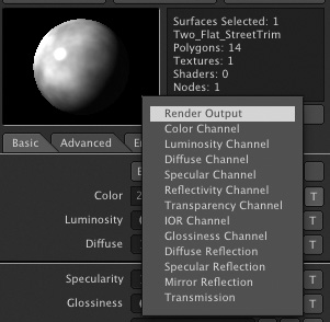
By default, the preview window (Figure 3.9) shows how your surface will look with all your surface settings applied collectively. You can use the Display drop-down to switch from this mode (which is called Render Output) to preview the effects of each attribute setting in isolation.

Figure 3.9. The Display drop-down list’s default option, Render Output, shows the collective results of all surface-attribute settings in the preview window.

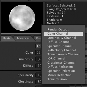
When you need to focus only on color, for instance, choose Color Channel from the Display drop-down (Figure 3.10) and you’ll see only the color component of the surface, rather than a complex surface with specularity, bumps, and more.

Figure 3.10. The same surface in the Display window with Color Channel selected. Notice that the bump texture and specularity do not display as in Figure 3.9.

You can change this display to any surface aspect you want to concentrate on, such as transparency, glossiness, or reflection. If you are using a procedural texture for luminosity, for example, you might want to display just Luminosity Channel. The choice is up to you. Most commonly, this value can stay at Render Output, but you have the control if you need it.

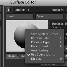
Click the Options button to the right of the Display drop-down to display a panel that lets you use a cube instead of a sphere as the preview object. The Options button also allows you to change the preview window’s background and lighting effects.

The Preset Shelf

Building surfaces is fun, no doubt, but seeing results right away can be even better. The Preset Shelf, a visual browser for surfaces, comes loaded with hundreds of prebuilt surfaces you can apply instantly to your models. (It also holds other types of preset attributes, such as camera handlers and environment handlers.)

To sample the prebuilt surfaces in the Preset Shelf, make sure the Surface Editor panel is open and choose Presets from the Windows drop-down, or just press F8. In the Surface Preset window that appears (Figure 3.11), click the Library drop-down (labeled WorkSpace, the default name for a new empty library) and choose the Rock surface library. These presets were installed when you installed LightWave 10.

Figure 3.11. The Surface Preset panel is home to hundreds of readymade surfaces, as well as any you decide to add.

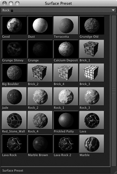
To copy a surface setting from the Surface Preset panel to another selected surface, first select the new surface name in the Surface Editor panel and then double-click in the preset surface in the Surface Preset panel. Also, double-click in the preview window to use the Save Surface Preset function. Be sure to have the Preset window open to see the saved surface. Double-click that surface preset to load it to a new surface. Similarly, you can right-click in the preview window for additional options, such as Save Surface Preset. To save a surface to the Preset Shelf, double-click the Display window in the Surface Editor, and the currently selected surface will be added to the library.

If you right-click in the Surface Preset panel, you can create new libraries for organizing your surface settings. You also can copy, move, and change the parameters.

Setting Up Surfaces

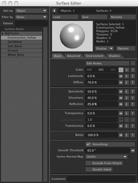
The main functions you use to set up and apply surfaces in the Surface Editor occupy four tabs: Basic, Advanced, Environment, and Shaders (Figure 3.12). Each controls specific aspects of a selected surface. This chapter introduces you to the most commonly used tabs, Basic and Environment.

Figure 3.12. Surface Editor controls are organized in four tabs.

Basic Tab

Aptly named, the Basic tab is home to all your basic surfacing needs. It’s here that you start most surfacing projects (Figure 3.13).

Figure 3.13. The Basic tab in the Surface Editor is home to the most commonly used surface settings.

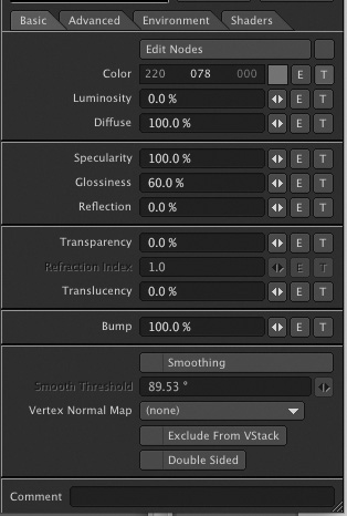
Within the Basic tab, you’ll find the following controls arranged from top to bottom:

• Edit Nodes. This feature allows you to control surfaces in an entirely new way. You would click this button and use it instead of the basic Surface Editor. This feature will be introduced shortly.

• Color. Here, you can set the color of the selected surface by entering values from 0 to 255 for each of three RGB (red-green-blue) or HSV (hue-saturation-value) color channels. Right-click in the number field to toggle RGB and HSV modes. Click and hold your mouse button on a channel’s numerical setting and slide the mouse right to increase the value or left to reduce it. Or just click the swatch to the right of the numerical field to open the standard color picker for your operating system.

To the right of the Color control, as well as the remaining controls in the Basic tab, you’ll find buttons marked E and T. Recall that E stands for Envelope—a function that enables a given surface-attribute value to vary over time. T stands for Texture, a function that lets you vary an attribute’s setting spatially, over the area of the surface. We’ll cover envelopes and textures later in the chapter.

The rest of the controls in the Basic tab work the same way. Each contains a number field you can click and type into in order to enter a setting. To the right of each number field is a LightWave adjuster called a mini-slider. To use one, click it and, holding down the mouse button, move your mouse left or right to change the setting value. The range of each mini-slider generally covers the observed values for that attribute in natural materials. Many controls let you type in values outside those naturally occurring ranges to achieve special effects.

• Luminosity. This controls the brightness, or self-illumination, of a surface.

• Diffuse. This is the amount of light the surface receives from the scene. You’ll learn more about this shortly.

• Specularity. This value specifies the amount of shine on a surface. High Specularity settings are appropriate for surfaces such as glass, water, and polished metal.

• Glossiness. Often confused with specularity, glossiness determines how shine spreads on a surface. A surface with high glossiness exhibits tight highlights or “hot spots”; this option is dimmed if specularity is 0.

• Reflection. If you want a surface to reflect light, you specify how much with this control; a mirror would have a high Reflection setting. When you want to control what’s reflected in a reflective surface, you’ll use the Environment tab.

• Transparency. This controls the degree to which you can see through a surface.

• Refraction Index. This value controls the amount that light bends as it passes through a transparent surface. Material with an index of 1 doesn’t bend light at all; the index for glass is about 1.5, and for water about 1.3. This control is dimmed on surfaces with zero transparency.

• Translucency. This value specifies the degree to which light can pass through a surface from behind, as it might a thin leaf or piece of paper.

• Bump. This controls a function that makes surfaces look irregular. It gives an illusion of surface bumpiness but doesn’t actually cause any elevation or depression of the surface geometry. The default setting is 100%.

• Smoothing. This shading routine, which is activated by default, makes surfaces consisting of polygons appear smooth. Deselect the check box to turn it off.

• Smooth Threshold. When smoothing is turned on, this specifies the sharpest angle between polygons that LightWave should try to smooth out. Generally, the default of 89.5° is too high. A typical beveled surface on a logo should have a threshold of about 30°.

• Double Sided. Check the box next to this option if you want selected polygons to exhibit surface attributes on both their front and back sides. Ideally, you don’t want to use this unless you have to. All models created in LightWave Modeler have their surfaces facing in one direction. This option fakes it and forces the surface to face the opposite way as well.

• Comment. Use this field to enter notes about your surface as reminders or to include more detailed descriptions. This is a great feature when you’re sending objects to colleagues and clients.

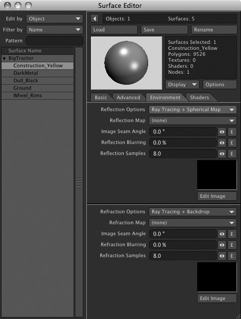
Environment Tab

Reflect for a moment on reflection. (Wow, that was lame!) If you look at an object and see a reflection, its contents aren’t determined by the object itself but by its surroundings, right?

In a 3D setting, surface reflections often include other models within a scene, and those reflections typically are created via a process called ray tracing, which generates reflections and shadows based on the location of objects and light sources within a scene. Reflections can also include images of objects that don’t exist as models in a scene; reflections of “offstage” objects or backdrops are created as 2D images, which you then overlay onto the reflective surface, a technique known as reflection mapping.

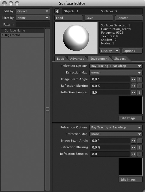
The Reflection attribute in the Basic tab controls how reflective a given surface will be; settings in the Environment tab (Figure 3.14 on the next page) control what appears in reflections generated by the surface. When you’re dealing with a transparent surface, the tab provides comparable control over how the surface refracts objects placed behind it in a scene.

Figure 3.14. The Environment tab gives you access to reflection and refraction controls.

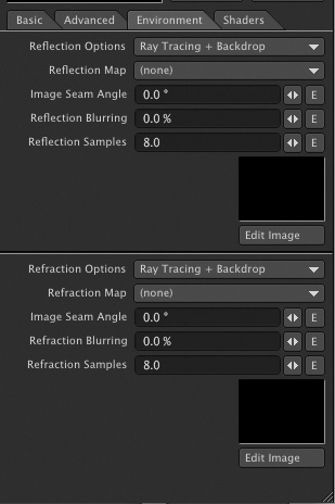
On the Environment tab, you can assign the following:

• Reflection Options: the type of reflection applied to a surface: spherical, ray trace, or backdrop

• Reflection Map: what image will be reflected

• Image Seam Angle: where the seam of a reflected image will appear

• Refraction Options: the type of refraction applied to a surface, either spherical or ray trace

• Refraction Map: the image file used (if any) for refraction

• Image Seam Angle: where the seam of a reflected image will appear

• Reflection Blurring: the amount of blur your reflections will have

• Refraction Blurring: the amount of blur your refractions will have

The best way for you to get a feel for using the Surface Editor and the Basic and Environment tabs is to try them out for yourself. An excellent way to observe the effect of the settings you choose is to use LightWave’s new VPR feature.

Working with VIPER

VIPER stands for Versatile Interactive Preview Render, and it gives you a preview of certain types of adjustments you can make to your scene in Layout, such as volumetric settings and surface settings. It’s important to point out that because VIPER does not do a full-scene evaluation, some aspects of your surfacing are not calculated, such as UV mapping and shadows. This means that VIPER is limited in what it can show. However, it is very useful for most of your surfacing needs, such as specifying color and texture. As you adjust your surfaces, VIPER shows you what’s happening and how the surface will look in your scene, without the need to re-render the whole scene. VIPER is available in Layout only.

Exercise 3.1. Working with VIPER and VPR

---

To get an idea of how useful VIPER is, try this quick tutorial.

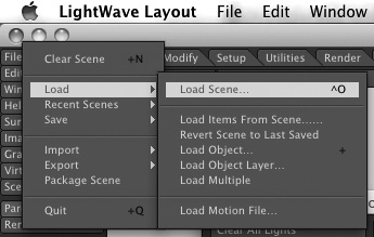
1. Start Layout, or if it’s already running, save any work you’ve completed so far and choose Clear Scene from the File drop-down menu (keyboard equivalent: Shift+N).
2. Choose Load Scene from the Load drop-down and open female_head.lws (located in the CH3 folder, inside the 3D_Content folder provided on this book’s DVD). You’ll see a 3D human female head.
3. Press F5 to open the Surface Editor panel.
   

   You’ll use VIPER to preview changes made in the Surface Editor, which must be open for VIPER to render and display the surfaces you set.

   Note

   You don’t always need to clear the scene before loading a scene. Simply loading a scene overrides your current scene. This two-step process familiarizes you with the available tools and Layout’s workflow.

4. Click Layout’s Render tab, and then click the VIPER button in the Utilities tool category. When you do, the VIPER preview window opens and the Enable VIPER button (in the Render tab’s Options tool category) is activated automatically (Figure 3.15). Press F7 in any Layout tab to accomplish the same thing.
   

   Figure 3.15. The VIPER command is found in Layout only, in the Render tab.

   

   When you click VIPER in the Render tab or press F7 to open the VIPER window, VIPER is enabled automatically. Repeating either of those operations closes the window but leaves VIPER active until you toggle it off using the Enable VIPER button—something you may want to do before running full frame or scene renders.

   Note

   Here’s the lowdown on the two VIPER-related buttons in Layout’s Render tab: The Enable VIPER button makes VIPER pay attention to the rendering buffer, which allows it to preview surface changes in its Display window. The VIPER button opens and closes the VIPER window. Disabling VIPER with the toggle button allows you to leave the VIPER preview window open but frees up system resources to speed frame and scene renders.

5. With the VIPER window now open, click the Render button at the bottom of the VIPER panel. An error message appears stating that VIPER has no surface data to render.
   

   This is normal. For VIPER to work, it needs you to render a frame so that it can store information from a buffer. Otherwise, VIPER has no idea what’s in your scene.

6. Click OK to close the error window, and then press F9 to render the current frame.
   

   This renders the current frame and stores the information in LightWave’s internal buffer and lets you see surface-setting changes through VIPER.

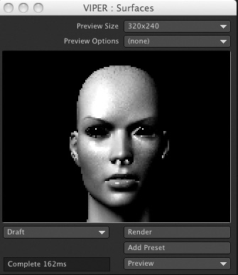
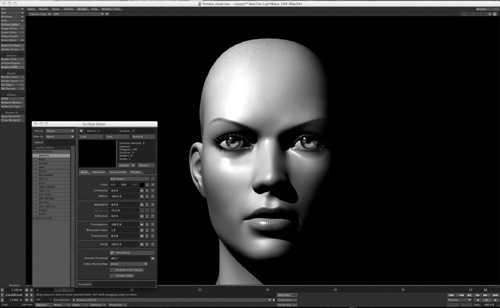
7. After the frame renders, press the Escape key (Esc) to close the Render Status window. If it’s in your way, move the Image preview window to one side. Then, in the VIPER window, click the Render button again. Do you see anything? The render you just created is now appearing in the VIPER window. Figure 3.16 shows the VIPER window, with the full Layout shown, once it has loaded and stored render settings such as Specularity, Diffuse, and Color. The previews in the VIPER window and Surface Editor’s preview window differ somewhat because Surface Editor’s preview uses a standard perspective or orthographic view of your object, while VIPER previews the scene from the viewpoint of your selected camera (thereby mimicking your intended results more closely).
   

   Figure 3.16. Pressing F9 on the keyboard renders the current frame and lets you preview surface changes through VIPER.

   

   Note

   It doesn’t matter with a simple “scene” like this, but for more complicated scenes, you might want to disable VIPER while rendering the frame, then turn it back on before continuing.

8. In Surface Editor, choose “skin lips” from the Surface Name list. To see the surface name, you may need to click the white triangle to the left of the object’s name.
9. To quickly see VIPER’s interactivity, click the mini-slider to the right of Diffuse in the Surface Editor’s Basic tab. Hold down the mouse button and slide your mouse to the left to take the value down to 0, and then release the mouse button. You’ll see the VIPER window update, to make the lip area appear black. What you did was tell the surface not to receive any light from the scene, essentially turning off the lights for that surface. A Diffuse value of 0% means light is not diffused, or transferred to the surface.
   

   Note

   You may think to yourself, “But Dan, I didn’t set up any lights for this scene, so how can the object receive or not receive light?” Remember, Grasshopper: Every default LightWave scene has one camera and one light. Aha!

10. Now, restore the Diffuse value to 100% and continue.
    

    You’ll see various surface settings appear throughout the commands on the right, on the Basic tab.

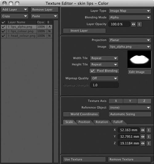
11. Click the T button to the right of the Color control to open the Texture panel for the skin lips surface (Figure 3.17).
    

    Figure 3.17. Clicking any of the T buttons throughout LightWave, including the Surface Editor, opens the Texture Editor.

    

    Note

    If the T button to the right of the Color control is dimmed, deselect the Edit Nodes check box located immediately above it.

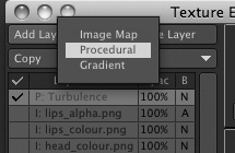
    You’ll see that the Layer Type drop-down at the top of the commands is set to Image Map—a setting that lets you apply images to a surface and much more, as we’ll see later in the book. For now, select Add Layer and choose Procedural, as in Figure 3.18. Deselect the three image map layers.

    Figure 3.18. The default Texture Editor layer type is Image Map. Change this to Procedural instead.

    

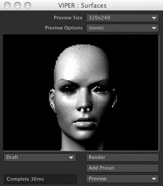
    Procedural textures have no seams, and are often just what the doctor ordered for organic-looking surfaces. Their surface attributes vary via mathematical procedures; each procedural type yields a different effect. By changing procedure settings within the Texture Editor and combining procedural textures in various ways, you can create a limitless range of organic surfaces. However, with a selected range of polygons, such as the lip area, a procedural texture shows the seam of material area. The benefit is, VIPER shows you the good and bad of adding and editing surfaces, helping your workflow.

    The Procedural Type is set to Turbulence, a variation of fractal noise that has been used by LightWave animators for years. Adding Turbulence as the Procedural Type to the current surface color of the lips, which is a pale color, adds variances to the surface, especially if the procedural color is offset to a color like blue.

    The Blending Mode is set to Normal, which tells LightWave to add this procedural texture to the selected surface. (Other Blending Mode settings are used when you apply multiple textures to a surface; they determine how textures combine with each other.)

    The Layer Opacity is set to 100%, telling LightWave to use this procedural texture to the fullest extent.

12. Make sure the VIPER window is open and visible to the side of the Texture Editor.
    

    If VIPER is not open, click the VIPER button (not Enable VIPER) in Layout’s Render tab. You rendered the scene in step 5, and LightWave remembers that by storing the data in its internal buffers.

13. With the Texture Editor and VIPER open, you can make changes to surface settings and see your changes in real time. Figure 3.19 shows the VIPER panel.
    

    Figure 3.19. Once you’ve made a render of a frame (by pressing F9), VIPER can now display the render, and you can make surface changes in the Texture Editor (among other places) and see them in real time.

    

    Note

    The VIPER preview window has default size of 320 × 240 pixels. You can expand it to 480 × 360 or 640 × 480 pixels using the Preview Size drop-down. Adjust the preview window to suit your screen size. When you do so, there’s no need to re-render your image. However, if you change scene lighting or object position, or add or remove objects in the scene, you need to re-render by pressing F9.

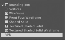
14. Make certain that the Texture Editor is still open (you get to the Texture Editor by clicking the T button next to Color in the Surface Editor). Next, close the VIPER window. Then in Layout, click the drop-down menu at the top of the interface and change from Texture Shaded Solid view to VPR, as shown in Figure 3.20.
    

    Figure 3.20. To activate VPR mode, just select it as a viewport option.

    

15. Back in the Surface Editor, make sure the Texture Editor panel is open. Now, because the procedural turbulent noise texture was a little too heavy, go ahead and delete it by first selecting it in the Layer Name list and then clicking Remove Layer at the top of the Texture Editor.
16. Next, turn the three layers back on by clicking the check marks to the left of the layers. Take a look in the main Layout window. How does that look? Amazing, right? A real-time render directly in your interface. Figure 3.21 shows the interface with VPR active. Cool, right?
    

    Figure 3.21. Changes to texture-property values such as Color, Scale, and Contrast are easy to see with the VIPER window open.

    

VIPER and VPR will quickly become your best friends when you’re working with LightWave Layout because they save you time. Not only that, many of you may not be mathematical wizards and do not care to calculate every value within the surface settings. Using VIPER can answer many of your questions when it comes to surfacing, especially when using Hypervoxels for particles (discussed in Chapter 10), because you can instantly see the results from changed values. VPR is terrific for interactively working “in” your scene. Using these tools will guarantee that during your 3D work, you’ll make a change to a value or setting and utter a loud “Oh, that’s what that does!” from time to time.

VIPER and VPR Tips

Here are a few more VIPER and VPR tips before you move on:

• Never trust VIPER as your final render. If something looks odd, always make a true render (by pressing F9 or F10) to check final surfacing.

• You can use VIPER to see animated textures by selecting Make Preview from the Preview drop-down list in the VIPER window.

• Press the Escape key (Esc) to abort a VIPER preview in progress.

• Click Draft Mode in the VIPER window to reduce redraw time (and render quality).

• Clicking a particular surface in the VIPER window instantly selects it in the Surface Editor’s Surface Name list. This is a great feature and can save you a lot of time on complex textured scenes.

• VIPER is available only in Layout, not Modeler.

• VPR works quite well on most computers. Understandably, the more processing power you have, and the bigger your video card, the better your performance will be.

• VPR has many options that can help you work faster and more efficiently. Be sure to watch the VPR video on the book’s DVD to see all the features in action.

Common Surface Settings

To take you even further into the LightWave Surface Editor, try applying a reflection in Exercise 3.2.

Exercise 3.2. Applying a Reflection to a Surface

---

You may sometimes have a project that requires you to use a building, vehicle, machine, toilet, or something completely different from what you’re used to working with. This could be an object that you’ve created yourself, purchased, or downloaded from public archives on the Internet. Follow these steps to apply a simple reflection to a surface:

1. Be sure to save any work you’ve completed thus far. Start Layout, or if it’s already running, choose File > Clear Scene.
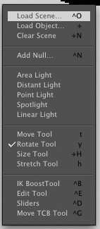
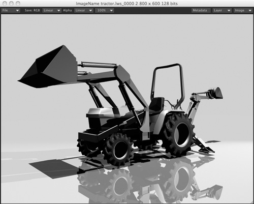
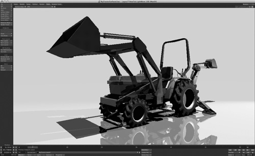
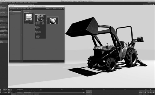
2. From the DVD that accompanies this book, load the BigTractor scene from the Chapter 3 projects folder in 3D_ContentScenesCH3. To load the scene, go to the Items tab, and then on the left side of the interface, click the Scene button under the Load category, as in Figure 3.22.
   

   Figure 3.22. Load the BigTractor scene into LightWave to set up some surfaces.

   

   Here’s a very handy tip: You can hide all the toolbars and menus in Layout and work with just the keyboard and mouse. Press d on the keyboard to access the Display Options tab of the Preferences panel. Select Hide Toolbar (Figure 3.23). Now, when in Layout, you can access the Surface Editor (or any other panel) by Control-Shift-clicking in the Layout window (using either the left or right mouse button). This pops up the list of commands and menus you’ve just hidden away (Figure 3.24)! Press d again to access the Display Options panel to unhide the toolbar. Now that you know where things are located, just use Alt+F2 to hide and unhide the toolbar. You can also open the Surface Editor quickly by pressing F5.

   Figure 3.23. The Display Options tab of the Preferences panel.

   

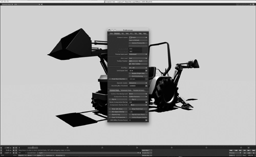
   Figure 3.24. The list of commands and menus you hid by selecting Hide Toolbar.

   

   Note

   Remember that you should be using LightWave’s default interface configuration for all tutorials in this book. To make sure you are, press Alt+F10 on the keyboard to call up the Configure Menus panel. Click the Default button from the Presets drop-down list at the upper-right side of the panel’s interface. If it is dimmed, you already have the default interface set. Click Done to close the panel.

3. After the scene has been loaded, click the Surface Editor button on the left side of the interface to open the Surface Editor panel. You should still be in VPR mode.
   

   You can see that by default, the object name appears in the Surface Name list.

4. If you don’t see all the surfaces, just click the small triangle to the left of the BigTractor filename and it will open the Surface Name list for that particular object.
   

   All the surfaces associated with the BigTractor object appear, as shown in Figure 3.25.

   Figure 3.25. When an object is selected in Layout and the Surface Editor is opened, the selected object’s surfaces are listed.

   

   Note

   If you have more surfaces than you do space in the Surface Name list, a scroll bar appears. Simply drag the scroll bar to view the entire surface list.

5. LightWave enables you to resize the Surface Editor panel simply by dragging the edge of the panel. Drag the bottom edge to stretch out the panel. You can collapse the panel by clicking the small triangle centered at the top of the interface, and you can simply select your surfaces from the Surface drop-down list.
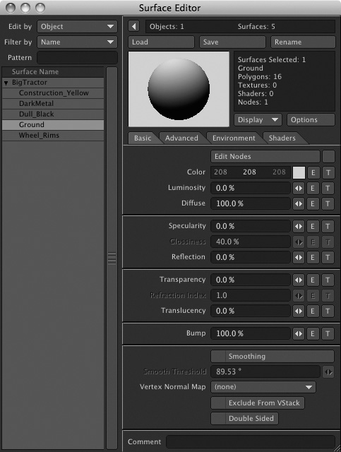
6. In Layout, make sure you’re in Camera view. You should be already, because the scene was saved this way before you loaded it. If not, switch to Camera view by selecting it from the drop-down list at the upper-left side of the viewport title bar. Then, select the Ground surface from the list within the Surface Editor.
   

   Note

   Naming your surfaces is half the battle when building 3D models. If you name your surfaces carefully, you’ll save oodles of time when you have many surface settings to apply. Organization is key! You name your surfaces in Modeler, as explained in previous chapters.

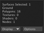
   When a surface is selected, the name appears in the information window to the right of the surface preview. The number of polygons associated with that surface also appears. In this case, the selected surface, Ground, has 16 polygons, as shown in Figure 3.26. You’ll also see a display at the very top of the surface panel that indicates the number of objects and surfaces in the scene.

   Figure 3.26. Summary information on the selected surface is displayed at the top right of the Surface Editor panel.

   

7. Because you simply can’t have a dull floor, you need to shine it up a bit. You know, make it look pretty. You can even make the ground look like glass or brass! First, you can change the color of the Ground but for now, leave it set to the default white. It’s set to the same color as the background so there’s a seamless transition.
   

   Here are a few tips for working with color values:

   • Clicking the small color square next to the RGB values makes the standard system color palette appear. Here, you can choose your color in RGB (red, green, blue), in HSV (hue, saturation, value), or from custom colors you may have set up previously.

   • Right-clicking and dragging the small color square next to the RGB values in the Surface Editor changes all three values at once. This is great for increasing or decreasing the color brightness.

   • Clicking the red, green, or blue numeric value and dragging left or right decreases or increases, respectively, the color value. You will instantly see the small color square next to the RGB values change. You’ll also see the sample display update.

   Note

   HSV represents hue, saturation, and value. It describes colors directly by their overall color, unlike RGB values, which are three discrete subcolors. HSV is another way to change color values. However, you might have more flexibility using RGB values.

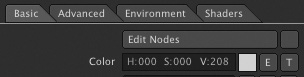
   • If you’re not keen on setting RGB values and prefer HSV values instead, rest easy. Right-clicking once on the RGB values changes the selection to HSV (Figure 3.27).

   Figure 3.27. Right-clicking any RGB value in the Surface Editor’s Basic tab changes the color-selection tool to HSV mode, and vice versa.

   

   • Make sure you’re using the display preview options as you like them. Right-click in the surface preview window to show more controls and options (Figure 3.28).

   Figure 3.28. Right-clicking in the surface preview window in the Surface Editor offers more control over how the surface is displayed. Here, you can set a checkerboard background, which is great for transparent surfaces.

   

With the Ground surface set to the soft white color, you still need to see the tractor reflected! You’ll need to make the Ground surface shiny. This next tutorial discusses surfacing the glass while introducing you to the rest of the Surface Editor. Remember that you will create many more surfaces throughout the chapters in this book, and that this is a brief introduction to just some of the features.

Exercise 3.3. Surfacing for Reflections

---

1. Make sure VIPER is opened and set off to the side of the Surface Editor so you can see your changes in real time. You can press F7 to open it. Or, keep VPR on! The choice is yours based on the speed of your system.
   

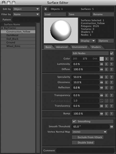
   With the Ground surface still selected as the current surface in the Surface Editor, go down the list of options and set each one accordingly.

2. Make sure that the value of Luminosity (the option just underneath Surface Color) is 0.
   

   Luminosity is great for objects that are self-illuminating, such as a lightbulb, candle flame, or laser beam. Note though that this does not make your surface cast light unless radiosity is applied, under the Global Illumination tab. This is in the Render Globals panel on the Render tab.

3. Set the value of Diffuse to roughly 60% to tell the glass surface to accept 60% of the light in the scene.
   

   The Diffuse value tells your surface what amount of light to pick up from the scene. For example, if you set this value to 0, your surface would be completely black. Although you want the glass to be black, you also want it to have some sheen and reflections. A 0 Diffuse value renders a black hole—nothing appears at all.

4. Set the value of Specularity to 40%.
   

   Specularity, in simple terms, is a shiny reflection of the light source. A value of 0% is not shiny at all, whereas 100% is completely shiny.

   When you set specularity, you almost always adjust the glossiness as well. Glossiness, which becomes available only when the Specularity setting is above 0%, is the value that sets the amount of the “hot spot” on your shiny (or not-so-shiny) surface. Think of glossiness as how much of a spread the hot spot has. The lower the value, the wider the spread. For example, Figure 3.29 (on the next page) shows two spheres, one with a low Specularity setting of 5% and Glossiness set to 15%. The result resembles a dull surface, like plastic.

   Figure 3.29. The sphere on the right has low Specularity and Glossiness settings, which results in a surface that looks dull. The sphere on the left, with high Specularity and Glossiness settings, looks more like glass.

   

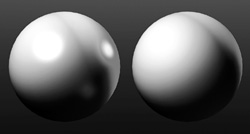
   On the other hand, the sphere to the right has a Specularity setting of 75% and Glossiness of 40%. The result looks closer to a shiny glass surface with reflections turned on. A higher Glossiness setting gives the impression of polished metal, or glass in this case. There will be a lot of surfacing ahead in this book for you, such as glass, metal, human skin, and more.

5. Now, back to surfacing the Ground in the BigTractor scene. Set the value of the Glossiness for the surface to 30%.
   

   This gives you a good, working shiny surface for now. Note, this is also a good formula for glass.

   Note

   It’s a good idea when setting reflections to make the Reflection value and the Diffuse value add up to roughly 100%. The current surface has Diffuse at 60% and Reflection at 30% for a total of 90%. This is not law, but just a guideline. If your Diffuse setting is 100% and you add a reflection of 40% or more, you’ll end up with an unnaturally bright surface.

6. Set the value of Reflection for the Ground surface to 40%.
   

   Most glass and clear plastic surfaces reflect their surroundings. In this case, the BigTractor is placed on a simple ground plane composed of just a few polygons. Just one basic Distant light illuminates the scene, along with one fill light.

7. You should now see the reflection showing up directly in your viewport. Because the Ground surface is flat, the Smoothing option is not necessary. If it were more round, you would want to turn Smoothing on. With objects that are more round, this option will take away any visible facets in the geometry.
   

   Note

   A shader is an algorithm that affects the surface properties of an object. It can change color, reflection, smoothing, reflectivity, and more. Shaders also can add special effects like procedural brick textures or fractal noise. The Smoothing setting employs a Phong shader. Developed by Bui Tuong-Phong in 1975, this shader works well on surfaces that emulate plastics, metals, and glass. Later when we get to the Node Editor, you’ll learn about LightWave 10’s other cool shaders.

8. Click the Environment tab within the Surface Editor panel (Figure 3.30).
   

   Figure 3.30. The Environment tab is where you set up reflection options in LightWave.

   

   Note

   Flatter surfaces are sometimes simply “too” smooth, and create odd renders. Reducing their smoothing thresholds can fix that.

9. Make sure Reflection Options is set to Ray Tracing + Backdrop, if it’s not already.
   

   This tells the surface to reflect what’s around it (in this case, an essentially bare set). If other objects were in the scene, they would be reflected too.

   Because LightWave can calculate reflections, setting a reflecting image can often help create a more realistic surface. You’d do this for the tractor surfaces, to help them look like metal. Glass-like surfaces, on the other hand, should reflect their surroundings, so ray tracing is used.

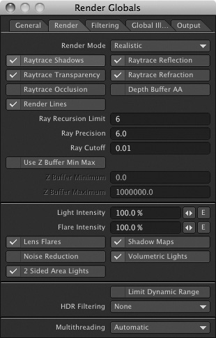
10. For ray-traced reflections to work, you need to tell the render engine to calculate this feature. If you don’t see a reflection currently, and VPR is on, click the Render tab at the top of the screen and then open the Render Globals panel. Make sure under the Render tab (within the Render Globals panel) that the Raytrace Reflection option is on, as well as Raytrace Shadows. This will tell the render engine to calculate reflection and shadow rays, as in Figure 3.31.
    

    Figure 3.31. For ray-traced reflections to work for a surface, you must tell LightWave’s renderer to calculate them.

    

11. Press F9 for a single frame render. While you’re in the Render Options panel, make sure Render Display is set to Image Viewer (in the General tab) to see a pop-up of your rendered image. Figure 3.32 shows the render.
    

    Figure 3.32. The Ground surface is very reflective, but the F9 render looks like the VPR in Layout.

    

    What’s that? VPR is so powerful that you can see your full render right in Layout, so often the typical F9 preview render is not necessary.

12. Choose Save All Objects from the Save submenu in the File drop-down. This saves the surfaces you’ve just set. Then, choose Save Scene from the same Save submenu to save the lighting, ray trace settings, and so forth. Now it’s time for the metal!

Creating Metallic Surfaces

You might think it would be difficult to match the real-world properties of metal on any objects you create, even a few balls. Believe it or not, this is easy to do within LightWave 10. The right amount of color, specularity, glossiness, and reflection helps create the visual effect. You’ve created the transparent glass surface, so how about something completely different? In this particular instance, a metal surface could work very well. This same metal can be applied to almost any metallic surfaces you create—from logos, to machines, to fasteners—with only minor variations. This section takes you through the steps required to create a metal surface.

Exercise 3.4. Creating a Metallic Surface

---

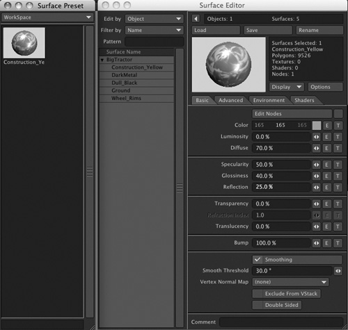
1. In the Surface Editor, select the Construction_Yellow surface. Set the color to a soft gray to simulate a silver metallic surface. Try setting all three RGB values to 180.
2. Set Diffuse to 70%, Specularity to 50%, and Glossiness to 40%.
3. A reflection is needed, so set Reflection to 25%.
   

   At this point, the surface doesn’t look much different than when you loaded it, other than a color change. Remember that other factors, such as surroundings and lighting, play a role in surfacing, but you still need to apply the reflection environment. Figure 3.33 shows the surface settings.

   Figure 3.33. Metal surfaces begin with basic color properties and a low Glossiness setting.

   

4. With the Construction_Yellow surface still selected, click the Environment tab (to the right of the Basic tab).
5. Set Reflection Options to Ray Tracing + Spherical Map, as in Figure 3.34. This tells the surface to reflect not only what’s around it but an image as well.
   

   Figure 3.34. The Ray Tracing + Spherical Map setting is a great way to make realistic metallic surfaces.

   

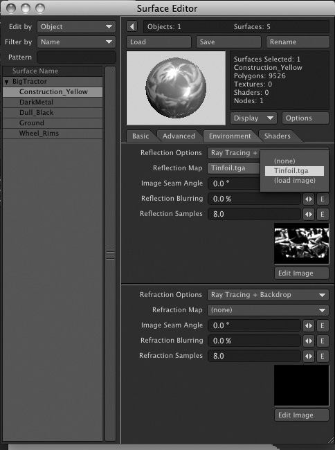
6. For the Reflection Map option, click the drop-down and select Load Image, as in Figure 3.35. Load the image named Tinfoil.tga from this book’s DVD.
   

   Figure 3.35. You can load an image directly from the Reflection Map drop-down in the Environment tab.

   

7. Guess what? That’s about it for this surface! No need to press F9 to render a frame and see how it looks. Just check out the scene directly in Layout. Figure 3.36 (on the next page) shows the new surface applied to the tractor.
   

   Figure 3.36. Adding ray-traced reflections and a reflection image to a gray surface helps sell a metallic look for the area under the glass.

   

   It’s subtle, but effective. Experiment a little and see how more reflection looks, a little less, and even add a little Reflection Blur from the Environment tab to change it up.

From this point, you can work with any other object surfaces you like, and apply similar metals, glass, or your own combination of both. You can even select all but the glass surface and change the basic gray color to a yellow-orange, and you’ve now made gold. All the other surface settings still apply.

A few final thoughts on surfacing with reflections: Many factors come into play, such as the glancing angle of the camera, light, and shadows. The angle of the camera in the previous steps could have been moved to reveal more of the reflection. You can also try changing the metal reflections to just a spherical map in the Environment tab, rather than using the Ray Tracing + Spherical Map setting. This tells the surface to reflect only the image.

You’ll often come across situations where you need to use the same surface settings on multiple surfaces, such as in the previous exercise. With so many variables being set within the Surface Editor, keeping track of identical surfaces could be a problem. Not to mention, you might want a quick reference to the changes you’ve made to the current surface. This is where the Preset Shelf comes in, to save a surface.

Exercise 3.5. Saving a Surface

---

If you set up a surface you’d like to keep, you can simply save it in the Preset Shelf. To do this, follow these steps:

1. Make sure the Preset Shelf is open by clicking the Windows drop-down menu and choosing Presets. Then in the Surface Editor, select the Construction_Yellow surface (which you’ve now changed to gray). Double-click the display preview at the top of the Surface Editor.
   

   You’ll see that surface sample appear, with its settings now saved, in the Preset Shelf (Figure 3.37).

   Figure 3.37. Double-clicking the display sample in the Surface Editor, shown on the right, instantly adds those surface settings to the Preset Shelf, shown on the left.

   

2. Select the second surface you need to apply surfacing to, such as the Ground surface, in the Surface Name list.
3. Go back to the Preset Shelf and double-click the sample you recently added.
   

   A small window appears, asking you to load the current settings. This is asking if you want the settings from the Preset Shelf sample to be applied to the currently selected surface in the Surface Editor. In this case, you do.

   Note

   Although double-clicking the sample display is one way to add a surface to the Preset Shelf, you can also right-click the preview window and select Save Surface Preset. You can also just press the s key while in the Surface Editor. Finally, you can click Add Preset in the VIPER window.

4. Click Yes, and all the surface settings are applied from the preset to the selected Ground surface. For any small changes, adjust as needed in the Surface Editor.

By using a preset to copy and paste a surface, you’ll find it’s much easier to change one simple parameter, such as reflection, than it is to reset all the surface and reflection properties again.

As you can see from the previous examples, it’s not too hard to create simple, good-looking surfaces. The next step is to continue surfacing on your own, using the few simple parameters outlined in the previous pages. Color, diffuse, specularity, glossiness, and reflection form the base for nearly all the surfaces you create. After you have a handle on setting up the basics, read on to learn about the Node Editor. Now, there’s a lot more to learn about surfacing, such as texture mapping, bump mapping, and using procedurals for computer-generated textures. You’ll do this more throughout the projects in this book, but the information here should have you up and running with the basics of the Surface Editor.

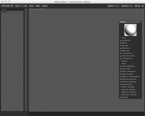
Introducing the Node Editor

Finally, we come to the Node Editor. You could, if you chose, use the Node Editor in place of the Surface Editor 100 percent of the time. That said, the Node Editor isn’t really meant to completely replace the Surface Editor. There are times when setting up a quick surface with the Surface Editor, as you’ve done with the exercises in this chapter, is simpler and more practical than firing up the Node Editor. But the Node Editor can help you take your textures and surfaces to the next level.

LightWave’s surfacing has been a layer-based system up until now. This system is still in place, but with the Node Editor, the rules have changed. Node-based texturing is found in many high-end 3D applications, because it allows you to create custom shaders, mix and match various surface properties, and much more. Unlike a layer-based system, the node-based system is like a network. Everything can connect and interact, from a simple surface to advanced materials. This next section will get you up and running with the Node Editor. Later in the book, you’ll create more advanced node-based surfaces. One last thing before the project: Although we’re discussing the Node Editor here in the chapter about surfaces, you should know that the Node Editor also exists for volumetric lighting and deformations. Of course, you’ll use these within the project chapters as well.

1. In Layout, save any work you’ve done. Reload the original BigTractor scene. Press F5 to open the Surface Editor. Select the Construction_Yellow surface listed in the Surface Name list. Then click the Edit Nodes button, as shown in Figure 3.38.
   

   Figure 3.38. Select the surface you want to change, and click Edit Nodes to open the Node Editor.

   

   Note

   To apply nodes to a specific surface, always select the surface in the Surface Name list. Be aware of this, as you might click the Edit Nodes button without thinking and apply node surfacing to the wrong surface.

2. When the Node Editor opens, position it as you like, and feel free to expand the size of the window by clicking and dragging the lower-right corner. Figure 3.39 shows the panel.
   

   Figure 3.39. The Node Editor open and positioned.

   

   Note

   If you can’t seem to pull any connections off a node, there’s a good chance you’ve sized down the view too much. In the upper-right corner of the Node Editor are move and zoom controls just like in Layout or Modeler. Click, hold, and drag these two icons to adjust the view.

3. The first lesson to learn is that there will always be a destination node. That’s the tall column you see in Figure 3.39. This node looks slightly different in the shading and texturing node (as you see here) than in the lighting or displacement node. Regardless, there will always be the destination node. Click and move it around to fit it to view. You can quickly do this by pressing the f key on your keyboard (f for fit—get it?).
   

   Note

   A destination node is what drives your render. In a sense, it’s the node, or part of the network, that outputs your other nodes.

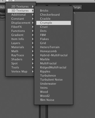
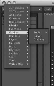
4. At the top left of the Node Editor is the Add Node menu. Select this and you’ll see a plethora of available nodes, from 2D and 3D textures, to gradients and cool shaders. For now, select 3D Textures, and then select Crumple, as in Figure 3.40.
   

   Figure 3.40. Adding a node is easy: simply select one from the Add Node menu. Here, a procedural Crumple node is selected.

   

5. It might be hard to wrap your brain around this way of texturing—that’s for sure. But don’t worry, you’ll get it. Just think of these nodes as ingredients that you can mix any way you want to create your final dish. Now, once the Crumple node has been added, it appears in the workspace area, as shown in Figure 3.41.
   

   Figure 3.41. The Crumple node added to the workspace area in the Node Editor.

   

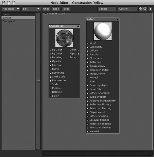
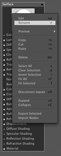
6. Taking a look at the preview thumbnail image at the top of the destination node (which reads Surface), it looks as if nothing has changed. This is correct. Nothing has changed. This is because even though you’ve added the node, you need to mix it in—that is, place it into the network. To begin getting organized, you can rename the default surface to something more specific. This is a good idea if you’re creating larger scenes. Right-click the surface name in the Node list and choose Rename, as in Figure 3.42. You’ll see that you can also access many other commands with a right-click (Mac users, Control-click).
   

   Figure 3.42. Right-click the surface name in the Node list to rename it.

   

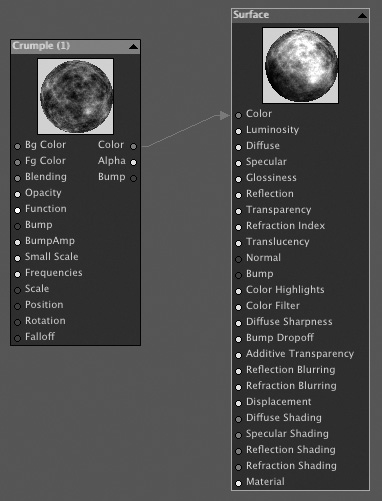
7. After renaming your surface, you’ll see that the destination node now shows the same name. The Crumple node needs to be connected to the destination node in some way. There are multiple ways to do this, and this is really the beauty of the Node Editor. For now, however, just click and drag the red dot for Color from the Crumple node, to the red dot for Color in the destination node. Figure 3.43 shows the result.
   

   Figure 3.43. To connect a node, click and drag from one node to the next.

   

   Guess what? You just used the Node Editor. It’s that easy! Of course, you simply added a single procedural texture, but the process is the same no matter what you’re creating. You add nodes and make the connections. Easy enough, isn’t it? So what’s the tough part? The tough part is understanding what connections to make and what all of the different nodes do. While we can’t cover every single node in this book, we can show you how to use and, more importantly, understand these different node connections so you can experiment on your own. On the book’s DVD is a video for you called “Node-Based Texturing” that will give you a good idea what the node editor is all about. And, you’ll perform more complex projects.

   Take a look at Figure 3.43, and you’ll see that the destination node preview shows the crumple surface applied. If you press F9 to render a current frame or simply look at the interface with VPR active, the crumple surface is on the tractor. The red arrow you dragged from the Crumple node to the destination node is a connection. There are five types of connections in the Node Editor. To identify each type of connection, NewTek has color-coded them. The red connection you just used is a color connector, and it has inputs and outputs, as you’ve seen. In most cases, you’ll connect color to color as you’ve done here, even though the Crumple node is mostly gray.

   Here is a list of the connection types:

   • Color. Receives input and outputs RGB color information. These connection types are designated by red dots on the nodes.

   • Scalar. Designated by a green dot, a scalar connection is a value. You can have inputs or outputs based on single values.

   • Integer. Great for blending, it is designated by purple dots. In most cases, integers connect to other integers.

   • Vector. Designated by blue dots, vector connections allow you to control different channels, such as position or rotation.

   • Function. This is a two-way connection, designated by a yellow dot. Function connections allow you to transform values of the nodes in which they are connected. You should connect functions to functions.

   Before you move on to the next chapter to learn about LightWave 10 lighting, let’s go a bit further in the Node Editor.

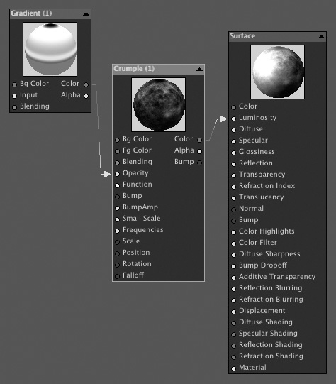
8. Back in the Node Editor, the crumple looks kind of dumpy applied with just a color connection. From the Add Node menu, select a Gradient node, as in Figure 3.44.
   

   Figure 3.44. A Gradient node will help add color and interest to the Crumple node.

   

   Note

   You can keep the info panel open for all selected nodes (rather than double-clicking one) by clicking the left-facing triangle in the upper-right corner of the Node Editor panel. This will open a numeric information panel that shows the info and preferences for any node when selected. Often, however, you don’t always need specific control for various nodes, so it’s closed by default. Certain node controls for things like a gradient can be opened by double-clicking the node itself.

9. A small node is added to the workspace. Now you need to connect this to the existing nodes. You need to build it into your network. Double-click the Gradient node in the workspace. A panel opens showing you specific controls for the node.
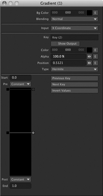
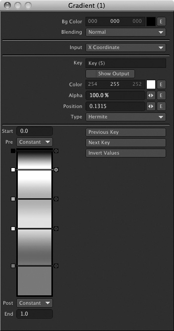
10. In the Gradient node panel that opened, you’ll see a tall black bar. A gradient allows you to vary settings based on different values. Click in the black bar, and a key is added. You’ll see a small line, as in Figure 3.45.
    

    Figure 3.45. The gradient controls allow you to vary different values, such as color. It begins by clicking in the gradient bar.

    

11. If you look carefully, you’ll see that this key you’ve added is actually now selected, and it is highlighted with a soft green. The default key is gray. With this new key still selected, change the color to red by clicking and dragging the value where it says Color in the panel. Figure 3.46 shows the area. Also, if you look at the Key listing in the panel, you can see that Key (2) is selected.
    

    Figure 3.46. Drag the red value to the right to set a red color to the added gradient key.

    

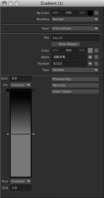
12. Now add another key. Click in the gradient bar to add the key, and then change the color to green by dragging the green value to the right. Remember, to change the RGB values, you can simply click and drag the numeric value. Or you can click the color swatch to open a color palette. Figure 3.47 shows the new key.
    

    Figure 3.47. Add another key to the gradient bar, and make this one green.

    

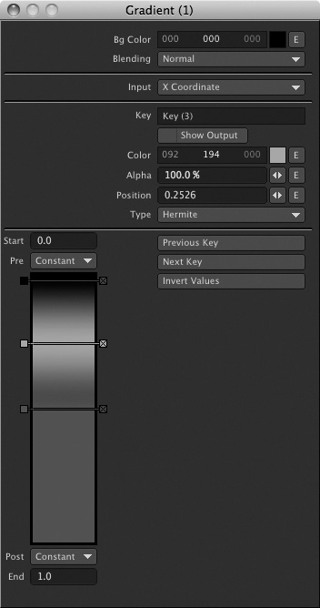
13. Go ahead and create two more keys, making one blue and one white. Figure 3.48 shows the final gradient. Note that you can click and drag on the keys to slide them closer together or farther apart to change how the gradient looks. Be careful, though; if you click off the key, most likely you’ll end up creating an additional key. To remove keys, click the right side of the key itself—there’s a small x. This will delete the key. You can add as many keys as you like.
    

    Figure 3.48. Add two more keys, one blue and one white.

    

14. Close the gradient panel. Back in the Node Editor workspace, you can see that your applied gradient shows in the node itself. Now all you need to do is connect it to the Crumple node. If you drag the Color channel from the Gradient node to the Luminosity input of the destination node, look what happens—the luminous values are changed for the destination surface. These are driven by the luminous output of the gradient. The green is brighter (has more luminance) than the red, and the destination node is updated accordingly, as in Figure 3.49.
    

    Figure 3.49. Taking the Color output from the Gradient node to the Luminosity input of the destination surface changes the values.

    

15. Try something different now. First, to “unhook” a connection, just click the arrow to remove it. Take the Color output of the gradient and connect it to the Opacity input of the Crumple node. Just click and drag the red dot, and then drop it on the Opacity input.
    

    Note

    You don’t have to move the nodes around in order to connect them. The system will pull the arrows to wherever you want, but it’s not a bad idea to arrange the nodes in left-to-right fashion to help stay organized. Just click and drag the nodes around as you like, remembering to press the f key to fit them to view.

16. Take the Color output from the Crumple node, and connect it to the Luminosity input of the destination node. The result is the crumple texture applied and then falling off based on the color values of the gradient. Figure 3.50 shows the result.
    

    Figure 3.50. With the gradient’s color connected to the crumple’s opacity, and the opacity’s color connected to the luminosity of the destination node, the surface is created.

    

17. Go back into the gradient controls. If you’ve closed the panel, double-click the Gradient node to open it again. Then, change the Input setting to Slope. By default, this value was set to X Coordinate, which is why the crumple was applied to the right side of the ball. Figure 3.51 now shows the Gradient node applied based on the slope of the object. Note that this change fed through the network you’ve set up. Cool, eh?
    

    Figure 3.51. Changing the gradient’s input setting to Slope also changes how the Crumple node is applied.

    

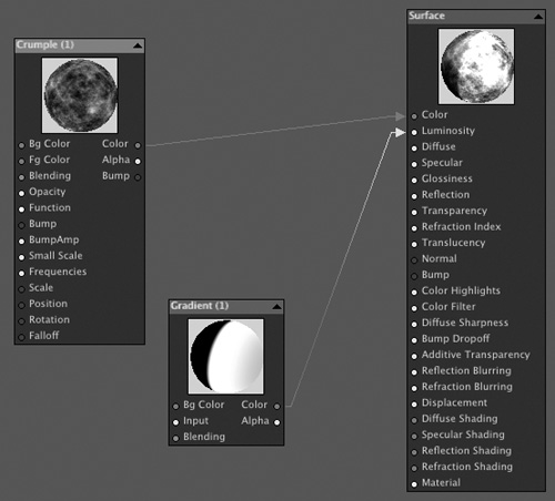
18. Here’s one more thing to try before you move on: Pull the Color output of the gradient to the Fg Color input of the Crumple node. This puts the gradient RGB values into the foreground color of the crumple texture.
19. Next, take the crumple’s Color output and connect it to the Color input of the destination node. Figure 3.52 (on the next page) shows the result: a gradient blended with the crumple.
    

    Figure 3.52. With the gradient Color output driving the foreground color of the Crumple node, the result is a blended surface.

    

Clearly, this is just the tip of the iceberg when it comes to using the Node Editor. As you experiment and progress in learning LightWave, you’ll use the Node Editor for more complex surface techniques, including lighting and deformations. And speaking of lighting, you’ll learn all about that in the next chapter!

The Next Step

From this point on, you can experiment on your own. Add more layers, play with gradients, and adjust procedurals. As a matter of fact, make as many additions and adjustments as you like. Your only limitations are time and system memory! Try adding some of the other procedural surfaces, such as Smokey, Turbulence, or Crust. Keep adding these to your rusty metal surface to see what you can come up with. Try selecting Copy All Layers from the Color Texture menu and applying them as Bump and Specularity textures. The results are endless. In addition, try applying LightWave’s powerful surface shaders.

This chapter gave you a broad overview of the main features within LightWave’s Surface Editor, including the Texture Editor. There are countless surfaces in the world around us, and it’s up to you to create them digitally. As the book progresses, you will use the information and instructions in this chapter to create even more complex and original surfaces, such as glass, skin, metal, and more. The next chapter takes you deeper into the power of LightWave—read on to discover the lighting and cinematic tools available to you.