
The vertical component of land developments is generally controlled by one of two Civil 3D features: surfaces or profiles. Surfaces cover the land-like sheets, defining vertical data as connections between points. (See Chapter 5, "Points.") Profiles handle vertical data as linear functions: a pair of station and elevation coordinates. Profiles define the model by providing the z-value, and an alignment provides the x- and y-values. In Civil 3D, profiles are tied to this relationship (with one pseudo-exception, the quick profile). In this chapter, you'll explore the profile as part of the road alignment layout and design.
This chapter includes the following topics:
Cutting a dynamic surface profile
Laying out and editing a design profile
Creating profile views to show the profile data
Superimposing profiles for design review
Labeling profiles along the profile and along the edges of the profile view grid
This chapter is titled "Profiles and Profile Views" because to Civil 3D, these are two distinct things. To Civil 3D, a profile is simply a list of coordinates—a station and elevation pair that make up vertical data along some alignment. The profile view comprises the grid, titles, labels, and data bands that display that information to you as a Civil 3D user. These two are intertwined, but you can show the same profile in multiple profile views with widely different settings for styles and labels to create a completely different representation of the same data. You'll look at the profile view in more detail later, but in this section, you'll learn about the two main types of profiles: surface profiles and layout profiles.
Surface profiles are the starting point for almost all profile creation, and creating a surface profile in Civil 3D is a straightforward process. Surface profiles are dynamically linked to both the surface and the parent alignment in Civil 3D, meaning that a change in either source data will force a change to the profile data. In this exercise, you'll sample the existing ground surface from the subdivision layout you've been working with, and then you'll create a simple profile view to display this information in a typical manner.
Open the
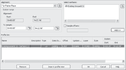
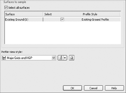
Surface Profiles.dwgfile. (Remember, all data files can be downloaded fromwww.sybex.com/go/introducingcivil3d2010.)From the Home tab and Create Design panel on the ribbon, select Profile → Create Surface Profile to display the Create Profile from Surface dialog shown in Figure 9.1.
Change the Alignment drop-down list to Parker Place. Notice how the Station Range area displays information about the selected alignment. You can also use the station boxes here to sample a limited range of stations along an alignment if you'd like.
Click the Add button at mid-right, and the Existing Ground (1) – Surface (1) profile will be added to the Profile List area as previously shown in Figure 9.1.
Congratulations, you've just completed sampling your first profile. Remember, profile data and profile views are not the same thing. To actually display this data in a form that makes sense, you need to draw in a profile view. You'll do that next.
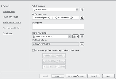
Click the Draw in Profile View button at the bottom of the dialog to close it and open the Create Profile View Wizard shown in Figure 9.2.
This is considered a wizard because it steps you through a number of different options in a linear fashion. Although you can jump from step to step using the links on the left of the dialog, you should follow the steps until you're more familiar with all of the options available. You'll generally accept the defaults, but walking through the wizard gives you a chance to see the location of many settings you might want to explore later.
In the General step, accept the default values and click Next. (You'll explore profile view styles in a later exercise.)
The Station Range step allows you to show a limited portion of the profiles if desired. Make sure the Automatic radio button is selected and click Next.
The Profile View Height step allows you to specify a specific height for your view, or to split views that have large vertical displacements so that they fit better into your sheet. Verify that the Automatic option is selected and click Next.
The Profile Display Options step allows you to select label sets for profiles, select whether or not to draw a profile on a given profile view, select a profile to use for grid clipping, and a number of other options that make it easy to get just the view you'd like. You're drawing a simple surface profile, so click Next to bypass the Pipe Network display (since there are no pipes in this drawing) and move to the Data Bands tab.
Data Bands are strips of data oriented along the top or bottom of a profile (or section) view that display relevant information based on the profile data at that station. They can be used to display two different surface elevations desired intervals, or to display the depth of a design profile, or perhaps to display the general shape of the horizontal geometry at that location. You'll adjust this later. Click Next.
The Profile Hatch Options step is new to Civil 3D 2010. It allows you to hatch areas of cut/fill, handle multiple boundaries on the profile, and perform take-off hatching. This allows better presentation of this profile. Examine the options, but do not make any changes. When you are done, click the Create Profile View button to dismiss the wizard.
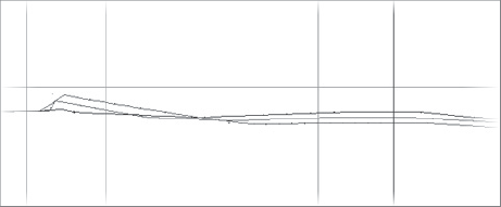
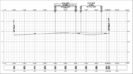
Pick a point in your drawing window somewhere to the east of the site. The profile view will be drawn as in Figure 9.3.

You'll notice that in the entire wizard, you didn't make any changes. Once you have Civil 3D configured and tweaked just how you like it, you'll be able to simply click the Draw in Profile View button right off the bat in the wizard, and skip all the settings tabs. By having all of those options preloaded, you can make it almost instantaneous to create a number of views just the way you need them.
One common development requirement is to show the ground surface at various parallel locations. In highway or subdivision work, this is commonly the right-of-way, and is a simple matter of adding offsets to the profile information, as you'll do in this exercise.
Open the
Offset Profiles.dwgfile (or continue working with the Surface Profiles drawing file if you completed the last exercise).From the Home tab and Create Design panel on the ribbon, select Profile → Create Surface Profile to display the Create Profiles from Surface dialog.
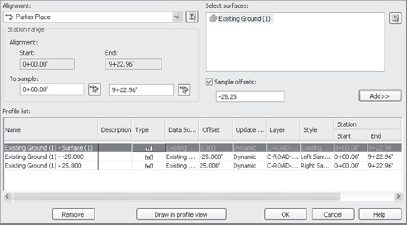
Select Parker Place in the Alignments drop-down list at the top-left. The Profile List area reflects the already existing profile.
Select the Sample Offsets check box to activate the offsets text entry area.
Enter −25,25 into the Sample Offsets box as shown in Figure 9.4, and then click the Add button to add the new profiles to the Profile List area. Note that you used a negative value to denote a left offset, positive to denote an offset to the right.
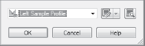
In the second row of the Profile List, click the Style cell to display the Pick Profile Style dialog shown in Figure 9.5.
Select the Left Sample Profile style as shown, and click OK to dismiss the dialog.
In the third row of the Profile list, select the Style cell again, and pick the Right Sample Profile style this time. By using different styles for left and right sample profiles, each will be visually distinctive.
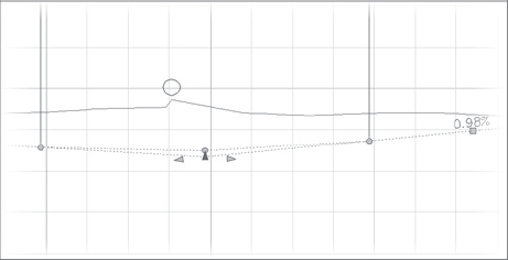
Click OK to close the Create Profile from Surface dialog and dismiss Panorama. You don't have to create a profile view this time because you already have one. Zoom in on the profile view to see the distinct profiles. Your screen should look similar to Figure 9.6.
If you zoom in close enough, you'll notice that the left and right profiles have small triangle-shaped markers at every point. That's a part of the style, and you'll look at modifying these markers (or making them disappear) in a later portion of this chapter.
As mentioned previously, the profile information is dynamically related to both the surface and alignment. If an alignment is lengthened, shortened, or simply relocated, the profile information is updated. In addition, any profiles that were created based on offsets are updated as well. In this exercise, you'll move the road centerline and see this relationship in action.
Open the
Dynamic Profile.dwgfile (or keep working with the same file if you've completed the prior exercises). Make sure you can see both the Parker Place alignment and the profile view.Select the alignment to activate its grips. Be sure to pick the alignment—picking a label will simply make it possible to drag the label away from the alignment!
Select the starting-point grip and drag it to the southeast. Pick a point near the location shown in Figure 9.7 to set a new starting location for the alignment. Notice that the profile view has lengthened and all of the profiles reflect this new alignment location as shown in Figure 9.7

This is obviously a temporary location, but the power shouldn't be underestimated. The ability to grab an alignment, manipulate it on screen, and instantly see feedback in the profile view is a powerful design iteration tool. Exploring and searching for vertically optimized design solutions is pick-and-click simple with this tool.
The same power can be applied to almost any object in Civil 3D. If you select a polyline in a Civil 3D drawing and right-click, one of the shortcut menu options is Quick Profile. Quick profiles give you the ability to get a look at your surfaces in a profile view without creating an alignment, sampling the surface, and creating a view. They're quick and easy, and you'll make one in the following exercise.
Continuing in the Dynamic Profiles drawing file, draw a line from the center of one cul-de-sac to another. (It doesn't really matter which two cul-de-sacs you use.)
Select this new line and right-click to display the shortcut menu. Select Quick Profile to display the Create Quick Profiles dialog shown in Figure 9.8. Here you can toggle on and off the surfaces to be displayed and the style they use, as well as what profile view style should be used.
Click OK to dismiss the dialog.
Pick a point on the screen, and dismiss Panorama. Civil 3D will draw a profile view similar to your typical profile view. Note that the title bar reflects a magic Alignment – (1) or something similar. Behind the scenes, Civil 3D is creating a temporary alignment and cutting a profile for you.
Move one end of the selected line to another cul-de-sac center point and watch the profile view update.
In this example, you used a line, but almost any object can be used to generate a quick profile. If you're not sure if a given object will work, select the object, right-click, and if the option is on the shortcut menu, you're in luck. Remember, while the quick profile is essentially the same as a typical alignment-based profile view of the given object cutting through surfaces, the profile view itself is a temporary object. This means that it will disappear the next time you save. That's great for designers, but don't build your construction documents with a quick profile, or you'll be left with nothing.
Close the drawing.
Once a profile of the existing ground has been created, it's time to begin designing the road by using a layout profile. Layout profiles are the design elements you'll use to design your roads, channels, and other vertical elements throughout Civil 3D.
Layout profiles are very similar to alignments in that they can be created simply by connecting points and adding in curves, or they can be created by laying in individual segments based on the idea of fixed, floating, and free elements. Because most users focus on profile design using a collection of PVIs (points of vertical intersection) and parabolic curves between tangents, you'll look at that design method in this exercise.
Open the
PVI Profiles.dwgfile. This drawing has sampled existing ground profiles for all of the site alignments already drawn into the model, and a collection of circles where you're going to place your PVI points.From the Home tab and Create Design panel on the ribbon, select Profile → Profile Creation Tools. At the
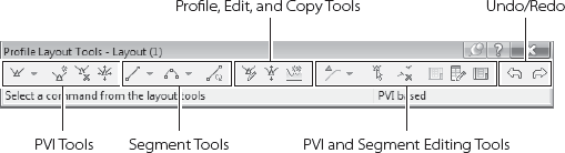
Select profile view to create profile:prompt, click the Parker Place profile view to display the Create Profile dialog shown in Figure 9.9.Change the label set to Complete Label Set as shown, and then click OK to dismiss the dialog. The Profile Layout Tools toolbar shown in Figure 9.10 will appear.
Similar to the Alignment Layouts Tools toolbar, the left portion of the Profile Layout Tools toolbar is for the creation of profiles, the middle segment is for adjusting and copying profiles, the next portion is for editing, and the last buttons perform the Undo and Redo functions.
Click the drop-down menu on the left and select Curve Settings to display the Vertical Curve Settings dialog. Here you can adjust the type of curve used by Civil 3D in profile designs (parabolic, circular, or asymmetric) and decide what parameters will drive those curves.
Change the length to 200′ for both Crest and Sag curves, and then click OK to dismiss the dialog.
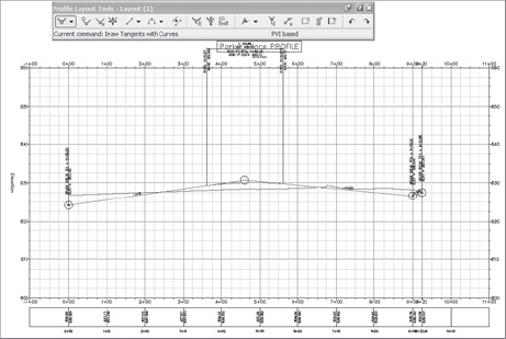
Click the drop-down menu on the far-left of the Profile Layout Tools toolbar again, and select the Draw Tangents with Curves option.
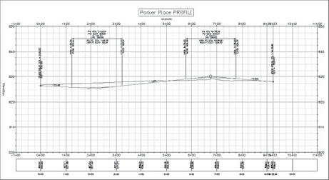
Turn on a center snap, and select the center point of the circles drawn in the Parker Place profile view grid. Right-click after the last circle to exit the command. Your screen should look like Figure 9.11.
Your first layout profile is complete. The circles were there to guide you, but you can place PVIs anywhere you see fit, just as when drawing an alignment in a plan. As you place PVIs, Civil 3D attempts to fit a parabolic curve based on the predefined settings; but if it cannot fit a curve of the length requested, it will simply skip the curve. To see this in action, zoom in near the right end of your profile and note that the last two segments are simply joined together with no curve between them.
Close the drawing

The act of creating an alignment with the most basic tools like this makes it quick and simple to create a number of alternatives, and to edit them as needed. Civil 3D allows the creation of multiple profiles defined as layouts, without requiring any of them to be designated as the primary profile. When you examine profile views in more detail in a later section of this chapter, you'll learn how to control which profile is displayed within a given profile view.
In the first exercise, you ignored the concept of design criteria. Civil 3D includes the ability to use design criteria as a control factor in laying out your design. AASHTO 2001 is built into the box, but you can create and manage your own criteria. Performing highway design (requiring the American Association of State Highway and Transportation Officials [AASHTO] guidance) is beyond the scope of this introductory level text, so now you'll move on to another creation methodology.
Creating a quick layout profile by picking random points as in the previous exercise is great for preliminary design, but when you are trying to tighten up a design, or trying to input a design based on handwritten notes or plans, you'll need to control the PVI location, profile slopes, and curve information at a more granular level. To that end, Civil 3D includes a series of transparent commands that allow the direct input of station and elevation data, length and slope data, or station and slope data. In the next example, you're going to input a design file based on the following criteria:
Start at 0+00 with an elevation of 826.5. Draw to station 5+00 at 0.5%. Draw 250′ at −1%. Tie back into the existing ground profile at the end of the alignment.
Here are the steps you need to follow:
Open the
Designed Profiles.dwgdrawing file.From the Home tab and Create Design panel on the ribbon, select Profile → Profile Creation Tools and click the Parker Place profile view to display the Create Profile dialog.
Verify that the Profile Label Set is on Complete Label Set and click OK. The Profile Layout Tools toolbar will appear as before.
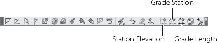
At this point, you need to make sure another toolbar is available, the Civil 3D Transparent Commands toolbar. If you have not modified your Civil 3D configuration, this toolbar is typically on the right side of the screen, and it looks like Figure 9.12. If you don't have this toolbar on your screen, you can access it by right-clicking in the gray dock area (but not on a button or toolbar) and selecting Civil → Transparent Commands.
Once you have the Transparent Command toolbar, you can proceed.
Click the drop-down menu on the left of the Profile Layout Tools, and select the Draw Tangents with Curves option. Civil 3D will prompt you to pick a start point. Instead of picking directly, you'll use the Transparent Commands toolbar.
Click the Profile Station Elevation button shown in Figure 9.12. Civil 3D will prompt you to select a profile view. Select the Parker Place profile view by clicking a grid line. A sliding jig will appear along the bottom of the profile view, indicating that a station selection is in progress.
Type 0 at the command line and press Enter. A jig will now appear along the vertical axis indicating an elevation selection is in place.
Type 826.5 at the command line and press Enter. Nothing will appear on the screen, and Civil 3D will prompt you to
Specify Station.Press Esc one time, and the prompt will change to
Specify End Point.Click the Profile Grade-Station button on the Transparent Commands toolbar, and the prompt will change to
Specify Grade.Type 0.5 and press Enter. Civil 3D will display a jig sliding along from the starting point and heading up at 0.5%, and then it will prompt you for another station input.
Type 500 at the command prompt and press Enter. Civil 3D will return to the
Specify Gradeprompt.Press Esc one time, and the prompt will change to
Specify End Point.Click the Profile Grade Length button on the Transparent Commands toolbar, and the prompt will ask you to specify a grade.
Type −1 at the command line and press Enter.
At the
Specify Lengthprompt, type 250 and press Enter.Press Esc one time to return to the
Specify End Pointprompt.Use an end snap and select the end of the existing ground profile that's already in the profile view. Press Enter to complete the command. Your screen should look like Figure 9.13.
Close the drawing.
By using the transparent commands, you can replicate existing data quickly and easily. Although it may seem like a lot of steps to produce this profile, familiarity breeds speed with the tools, and these transparent commands will become second nature very quickly as you work with profiles.
Once you've made a few profiles, the next step is to edit them. You'll look at that in the next section.
Editing profiles is similar to editing alignments as discussed in Chapter 8, "Alignments." Grip edits are the quick-and-dirty edits, but you also want to be able to manipulate PVI data more precisely, to adjust slopes, and to lengthen or modify curves. Just like other Civil 3D objects, edits made to the profile object are reflected almost immediately on the screen, along with all corresponding labeling. This means that searching for the perfect solution doesn't wipe out all the work you've done labeling, and makes it possible to explore alternative ideas in a time-efficient manner.
Grip editing is usually good for making initial design more palatable. Later on, as you look at corridors in Chapter 10, "Assemblies and Corridors," you will explore the interaction of profiles, corridors, and volumes. Being able to quickly manipulate a profile with grips and then rerun a volume calculation is invaluable in searching for the best engineering solution. In this exercise, you'll simply edit a profile using grips and the transparent commands again to refine a layout profile.
Open the
Grip Editing Profiles.dwgfile.Zoom in to the vertical curve near the 7+00 station and select the blue layout profile to activate the grips as shown in Figure 9.14. Notice that the ribbon now contains contextual information for only this specific profile layout.
Select the PVI grip (the vertical triangle) and, using a center snap, place it in the center of the small circle just to the northwest. The PVI will update, forcing a change in the curves, extension lines, labels, and data.
Pan to the left so that the grips for the curve near 2+00 are on your screen.
Select the PVI grip for this curve, but instead of picking a point directly, click the Profile Station Elevation transparent command.
Click the Parker Place profile view to select it.
Enter a station of 225 at the command line.
Press Esc to deselect the profile and zoom out. Your screen should look similar to Figure 9.15.
Close the drawing.
Moving beyond the quick grip edits, it's important to be able to precisely control the layout profile. Common review standards include using even station values for PVI points, and setting slopes to easy values. Although these requirements were more important when profile staking was a manually calculated process, it's still good design to follow these common rules. In this exercise, you'll fix a profile so that the PVI and slope data are more acceptable values.
Open the
Tabular Editing Profiles.dwgfile.Select the blue layout profile to activate its grips. Be sure to pick the profile, not one of the labels. Notice that the ribbon contains contextual information for only this profile layout.
From the Profile: Layout contextual tab and Modify Profile panel, select Geometry Editor. (You can also right-click and select Edit Profile Geometry from the menu.) The Profile Layout Tools toolbar will appear. (The same toolbar used to originally lay out the profile is used to edit the profile.)
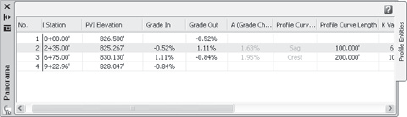
Click the Profile Grid View button near the right-hand side to display the Profile Entities tab in Panorama, as shown in Figure 9.16. This view allows you to see all of the data for the profile in one concise manner.
Click the PVI Station column for row 2 and change the value to 235.
Click the PVI Station column for row 3 and change the value to 675.
Click the Grade Out column for row 2 and change the value to 1.11%.
Click the Grade In column for row 4 and change the value to −0.84%.
Scroll to the right and click the Profile Curve Length column for row 2. Change the value to 100.
Click the X on the Panorama title bar to close the panorama, and close the Profile Layout Tools by clicking the red X and pressing Esc.
Close the drawing.
The direct input method allows you to drive certain PVI elevations based on whether you used the Grade In or Grade Out column. You may have to play a bit to get used to the way Civil 3D decides which parameters to hold while modifying others. At the end of the day, you can precisely design your profile to match whatever criteria you may need.
Moving points and adjusting grades is relatively simple, but adding to the profile, or adjusting the curves and tangent segments, is almost as simple. In many applications, making a change in the underlying geometry of the profile would mean scrapping the design and starting over. In Civil 3D, you use profile tools to simply add or remove PVIs and curves, as in this exercise.
Open the
Adding Profile Components.dwgfile.Select the Parker Place layout profile, and from the Profile: Layout contextual tab and Modify Profile panel, select Geometry Editor. (You can also right-click, and select Edit Profile Geometry to display the Profile Layout Tools toolbar). Remember, you can mouse over the tools to get their names as a tooltip!
Select the Delete PVI button. Civil 3D will prompt you at the command line to pick a point near that PVI to delete.
Click near the 4+75 station, and the PVI there will disappear, along with the curve.
Right-click to exit the command, and the labeling will update. Press Esc.
As you've seen, deleting and adding PVI information to an existing profile is as simple as two clicks. Adding a curve is almost as simple.
Select the drop-down menu next to the Fixed Vertical Curve button, and select the Free Vertical Parabola (PVI Based) option as shown in Figure 9.17.
Click near the PVI at station 6+75.
Enter 150 at the command line or press Enter to accept this default value. The curve will be added, but the labeling won't update.
Right-click to exit the command and update the labeling.
Close the drawing.

There are a number of different ways to build and edit profiles. Using these basic elements will handle a large portion of the profiles seen in land development work, and give you the ability to explore and play with profiles to understand your site design better. Now that you know how to create and manipulate profiles, you'll explore ways to display and label them in the next section.
To this point, you've been using a basic set of labels along the profile and around the profile view. Beyond the basics, there are styles in play for both the profile and profile view: labels and label sets for profiles, and data bands along the profile view. Because the profile and the profile view have distinctly different settings, you'll look at each in its own section.
Like most other Civil 3D objects, the profile object itself carries a style property reflecting how it will be displayed. Earlier in this chapter, you looked briefly at this option when displaying the left and right offset profiles, but it's important to review these styles and look at some options for their use. In this exercise, you'll modify the styles used in a profile view to reflect the change from a design mode to a plan production mode where extra information is added to meet review requirements.
Open the
Profile Styles.dwgfile.Select the layout profile in the Parker Place profile view, and from the Profile Layout contextual tab and Modify Profile panel on the ribbon, select Profile Properties. (You can also right-click and select Profile Properties.) This will display the Profile Properties dialog shown in Figure 9.18.
Switch to the Information tab if necessary and click the Object Style drop-down menu to display the available profile styles.
Select the Design Profile style from the list and click OK to dismiss the dialog.
Press Esc to unselect the profile. Note the change in the profile display.
Close the drawing.
As you can see in Figure 9.18, there's not much to a profile in terms of properties that would be modified. The style change in this case turned on the parabolic extension lines and changed the colors for the entire profile to be uniform as opposed to color-coded by element type. The use of a color-coded profile style is great during the design phase, and the ease of changing styles later makes it convenient to have styles for all kinds of uses and permutations.
The style of a given profile is often established during the creation of that profile, but labeling often comes as a later process. The labels a designer needs during the analysis and design stage often bear little resemblance to the reviewing agency requirements.
Thankfully, Civil 3D includes the concept of label sets for profiles just as in alignments, so making a change to the label set across a wide group of designed profiles is a relatively quick and painless task. In this exercise, you'll label one profile one component at a time, establish a label set from those choices, and then apply that label set to another layout profile in the drawing.

Open the
Profile Labels.dwgdrawing file.Zoom in on the Parker Place profile view and select the layout profile.
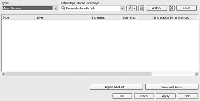
From the Profile: Design tab and Labels panel on the contextual ribbon, select Edit Profile Labels. (You can also right-click and select Edit Labels from the shortcut menu.) This will display the Profile Labels dialog shown in Figure 9.19.
Change the Type drop-down list to Grade Breaks, and then change the Profile Grade Break Label Style drop-down list to Station over Elevation if necessary.
Click the Add button to add this label to the profile. Note that the labels will not update in the model unless you click OK to close the dialog or Apply to push the changes out to the model.
Change the Type drop-down to Lines, and then change the Profile Tangent Label Style drop-down list to Percent Grade.
Click the Add button to add this label to the profile.
Change the Type drop-down list to Crest Curves, and then change the Profile Crest Curve Label Style to Crest Only.
Click the Add button to add this label to the profile.
Within the Labels table, select the Dim Anchor Val in the Crest Curves row, and change the value to 2.
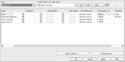
Change the Type drop-down list to Sag Curves, and then change the Profile Sag Curve Label Style to Sag Only.
Click the Add button to add this label to the profile.
Within the Labels table, select the Dim Anchor Val in the Sag Curves row and change the value to 2. Your dialog should now look like Figure 9.20.
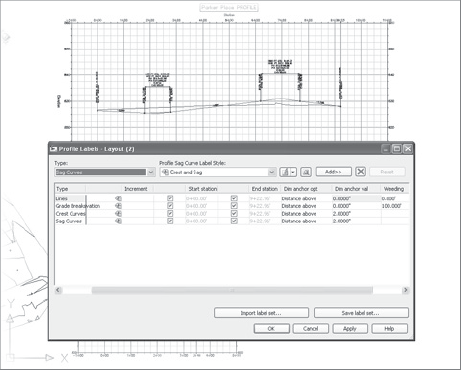
Click Apply to update your model. Your screen should look something like Figure 9.21. Note that the Profile Labels dialog is still open. Apply lets you see your changes in the model without leaving the dialog.
Click the Save Label Set button in the lower right of the Profile Labels dialog to display the Profile Label Set dialog.
Switch to the Information tab and change the name to Intro Roads.
Click OK to return to the Profile Labels dialog, and then click OK again to return to your drawing.
Press Esc to unselect the profile.
At this point, Parker Place is labeled as needed, but it sure took a lot of picks and clicks to get there! Thankfully, the label set you created in the last few steps of the exercise allows you to reapply those same selections quickly and easily to other profiles. In this exercise, you'll apply that label set, and then make a minor change to the destination profile labels to display all the points required.
Continuing within the Profile Labels drawing file, pan down to the Carson Circle profile view.
Select the layout profile and in the Profile: Layout contextual tab and Labels panel on the ribbon, select Edit Profile Labels. (You can also right-click to display the shortcut menu and select Edit Labels.) The Profile Labels dialog is displayed.
Click the Import Label Set button near the lower right to display the Select Style Set dialog.
Select Intro Roads from the drop-down list, and then click OK to close the Select Style Set dialog.
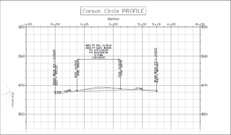
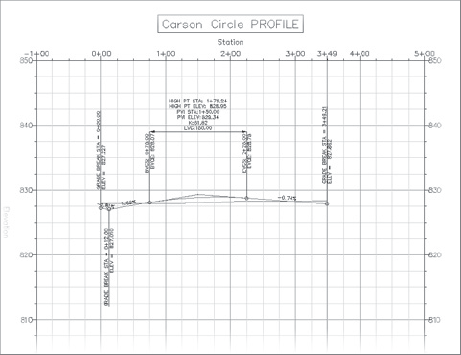
Click OK to dismiss the Profile Labels dialog. Press Esc. The Carson Circle profile view will look similar to Figure 9.22. Note that the PVI near station 0+12 is missing its label.
Select a label and right-click to display the shortcut menu.
Select Edit Labels to display the Profile Labels dialog again.
In the list of labels, click the Weeding column of the Grade Breaks row and change the value to 5. Weeding distances tell Civil 3D to ignore label points when they're too close together to make good-looking labels. In this case though, it's missing an important data point.
Click OK to dismiss the dialog, and the low point should now have a label.
Control-click on the new label to highlight the individual label instead of the label set.
Right-click and select Flip Label from the shortcut menu. Your screen should now look like Figure 9.23.
As you saw in previous exercises, the profile labels are dynamically tied to the profile geometry. Although the labels were applied in those exercises, there are also options for labeling Horizontal Geometry points or Major and Minor station points. Most people label these Major and Minor station elevations as part of the profile view, as you'll examine next.
Labeling profiles is important to review and design, but getting the display right is at least as important. Civil 3D makes it simple to have different grid displays for various uses and to show different pieces of information above and below the profile view as bands of data. Profile view styles control the grid lines and tick marks along the edges, the labeling on all four axis, and the title of the profile view and of each axis. Band styles control the display of information along the top or bottom edge of the profile view, and they can include information from simple elevations to complete data about superelevation. In this exercise, you'll manipulate multiple profile views and apply different styles and properties to control each view. Additionally, you'll see how to select which profiles are on and off within a particular profile view.
Open the
Profile Views.dwgfile. There are three Parker Place profile views in this drawing, and there is an alternate layout profile called Design 2 displayed in each of them.Select the top profile view grid and from the contextual tab and Modify View panel on the ribbon, select Profile View Properties. (You can also right-click to display the shortcut menu and select Profile View Properties.)
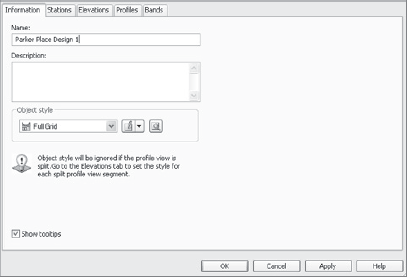
The Profile View Properties dialog is displayed as shown in Figure 9.24. Change to the Information tab if it is not already the active tab.
Change the Object Style drop-down list to Full Grid. The Information tab allows you to change the name of a profile view and change or edit the style in use.
Change the name of the profile view to Parker Place Design 1.
Switch to the Stations tab. The Stations tab allows you to specify a start and end station if you do not want to show the full alignment length in one profile view. This makes showing the profile view for a single sheet's worth of data very simple.
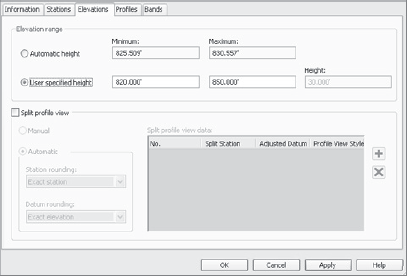
Switch to the Elevations tab. This tab allows you to modify the datum elevation, making it an even value, or to limit the height so that your profile views all have the same height.
Click the User Specified Height radio button to activate the Minimum and Maximum data boxes.
Enter 820 for a Minimum value and 850 for a Maximum value as shown in Figure 9.25.
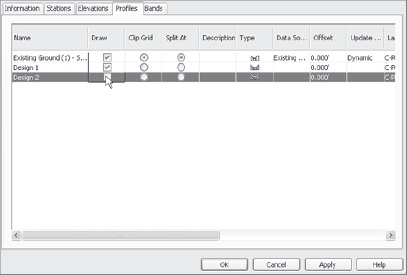
Switch to the Profiles tab and uncheck the Design 2 row under the Draw column as shown in Figure 9.26. This will not delete the profile data; it just toggles the display off!
Click OK to close the dialog. (You'll look at the Bands tab in the next exercise.)
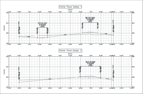
With this level of control, you can create multiple displays, using different grids and scales as needed. For practice, repeat the same steps on the middle profile view, changing the name to Parker Place Design 2 and toggling off the Design 1 profile. With that complete, your drawing will look similar to Figure 9.27. Remember, you still have the original view showing both design profiles at the bottom, and that a change to the profile objects in any view changes them all.
Close the drawing.
With the profiles in place, you may still need to show a bit more information. In this exercise, you'll add a pair of bands to a profile view, showing horizontal geometry at the top of your profile view grid, and elevation data along the bottom.
Open the
Profile Bands.dwgfile.Select the Parker Place profile view and from the contextual tab and Modify View panel on the ribbon, select Profile View Properties. (You can also right-click to open the shortcut menu and select Profile View Properties.)
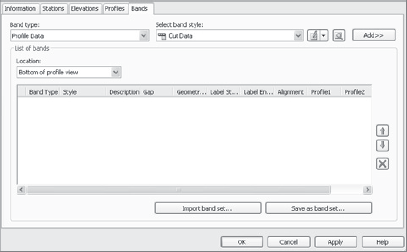
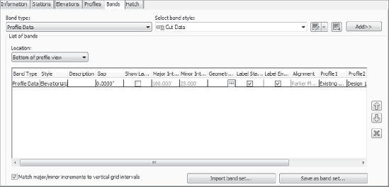
The Profile View Properties dialog is displayed. Switch to the Bands tab shown in Figure 9.28.
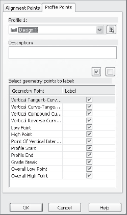
Change the Select Band Style drop-down list to Elevations and Stations, and then click the Add button to display the Geometry Points to Label in Band dialog. Under the Profile Points tab, change the Profile 1: selection to Design 1 as shown in Figure 9.29. The other dialog selections are somewhat irrelevant because the band is set up to label at major stations only.
Click OK to close this dialog and return to the Profile View Properties dialog.
Click the Gap column and change the value to 0.
Click the Profile 2 column in the first row, and change the drop-down list to Design 1. The Profile 1 and Profile 2 columns assign various profiles to various label components within the band. Your dialog should look like Figure 9.30 now.
Change the Location drop-down list to Top of Profile View. As mentioned, bands can be applied to both the top and bottom of the view.
Change the Band Type drop-down list to Horizontal Geometry.
Change the Select Band Style drop-down list to Geometry and click the Add button again.
Change the Gap value in the first row to 2. This will push the band information up above the title block for the profile view. Your dialog should now look like Figure 9.31.
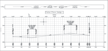
Click OK to close the dialog. Your profile view should look something like Figure 9.32.
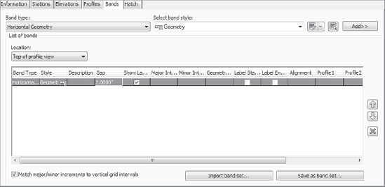
Figure 9.31. The Bands tab in Profile View Properties after a band is added to the top of the profile view
If you zoom in to the data band at the bottom of the profile view, you'll note that the elevations are different, reflecting the existing ground and layout profiles. This assignment was completed in step 7 of the preceding exercise. It's also important to note that the gap values entered are essentially offsets, pushing the band vertically away from a given axis. (You can use negative values here if you need to show something running inside your profile view grid.)
Close the drawing.
Although most of the time you'll be working with a single profile, it can be beneficial to understand the relationship between profiles in nonparallel situations. To assist in this understanding, Civil 3D includes a utility to superimpose profiles from one profile view to another. In the following exercise, you'll use this utility to compare the design profiles of two streets that run on adjacent blocks. This can be helpful when you grade the lots between them and need to know how much elevation difference you are covering. That's the case you'll examine in this exercise.
Open the
Superimpose Profiles.dwgfile. Carson Circle and Claire Point both have layout profiles drawn in the respective profile views.From the Home tab and Create Design panel on the ribbon, select Profile → Create Superimposed Profile. Civil 3D will prompt you at the command line to pick the source profile.
Select the layout profile in the Carson Circle profile view. Civil 3D will prompt you to pick a destination profile view.
Select the Claire Point profile view to display the Superimpose Profile Options dialog. The options here are handy if you'd like to show a portion of a longer alignment on the profile view of a shorter one, or just need to show a small range of stations for some reason.
Click OK to dismiss the dialog. The Claire Point profile view should look like Figure 9.33. Remember, the projection is a linear point projection, so distances and curves may look exaggerated in some way.
Remember, this is a dynamic link like so much else in Civil 3D. Modifying the design profile in the Carson Circle profile view will reflect in the Marie Court profile view. This gives you the real ability to quickly see how a profile is related to its peers.
Close the drawing.

Profiles and profile views in Civil 3D act together to give you a full measure of ways to display vertical information in your design. Sampled profiles that react to design changes allow you to design based on existing conditions, and they enable you to review alternate alignment placements in an instant. Layout profiles with smart elements that understand the relationship between the tangents and curves of the design and the labeling that comes along with them make design revision quick and even fun to do. Finally, profile views and bands give you full control of data represented in your construction documents, reducing the drudgery of plan production to almost nil.