© The Author(s), under exclusive license to APress Media, LLC, part of Springer Nature 2022
A. BoxIntroducing Charticulator for Power BIhttps://doi.org/10.1007/978-1-4842-8076-8_19

19. Taking It to the Next Level

Alison Box1  
(1)
Billingshurst, West Sussex, UK
 

Let me first congratulate you on having come this far. You’ve worked through all the chapters in this book, so you’re now an expert in generating visuals using Charticulator. It’s always been an implicit understanding that the reason you’ve invested your time and attention in learning how to use Charticulator is so you can design visuals that tell the story of your data, uncompromisingly and unequivocally and that can truly inform and persuade. This has been the overriding objective through everything you have learned about this inspirational chart generating software.

In this chapter, it’s time to prove that this objective has been achieved. It’s time to look at designing more ambitious visualizations that will use the skills you have learned in this book. We look specifically at how you can use multiple plot segments and glyphs, sometimes layered one on top of the other, to achieve truly customized visuals. Using this technique, you can mix and match chart elements in almost limitless combinations. We also look at how we can make use of DAX measures to control the display of chart elements or the formatting of those elements. This again is a method that can be applied to many different charting scenarios.

In what follows, I’ll be taking you through how to build the following visuals:
  • Matrix and card combination

  • Highlighted line chart

  • Categorized line chart

  • Jitter plot

  • Arrow chart

Matrix and Card Combination Visual

In Figure 19-1, we have designed a visual that combines a matrix style table with a summary card and comprises the following analysis:
  • Conditional formatting in the matrix to identify high and low sales values

  • A bar chart on the right to show subtotals for each region

  • A bar chart at the bottom to show subtotals for each year

  • A card on the right that provides a summary of the data

Figure 19-1

A visual combining a table, bar charts, and a card

This chart makes use of multiple plot segments, each with its own glyph. To generate the subtotals for each region and each year used by the bar charts and also the summary data in the card, we used Charticulator’s “Group by…” option.

The problem you will meet, however, is that you can only group by categories that exist in the underlying data, in our case by year or by region. To group by all the data so that you can calculate the aggregations in the card, you will need to generate a value that puts every row into the same category. I used a DAX measure to do this and named the measure “All,” populating it with a “Y”; see Figure 19-2.
Figure 19-2

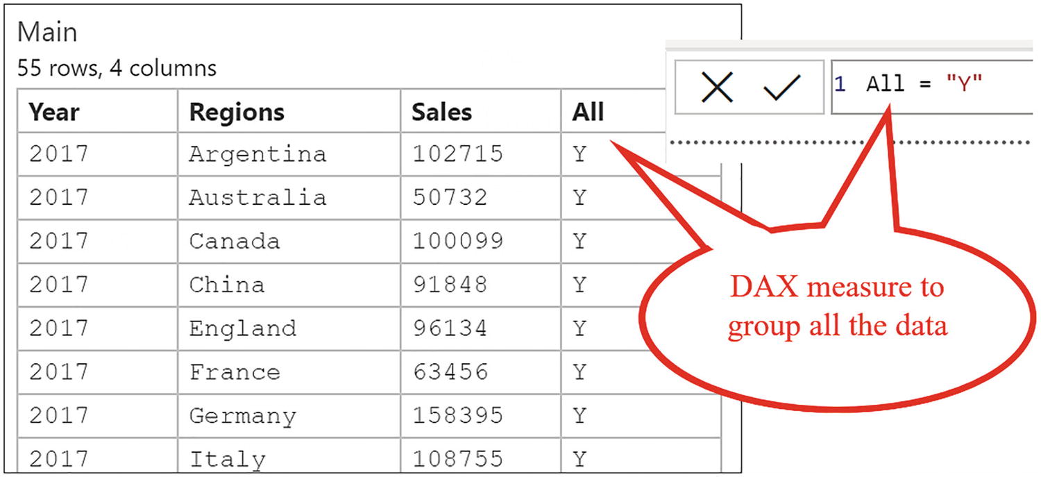
Create a DAX measure to group all the data

We are now ready to build the combination visual. In Figure 19-3, the four plot segments used in the generation of this visual have been set out.
Figure 19-3

The four plot segments used to generate the chart in Figure 19-1

You can see the guides that were needed to anchor each plot segment in the correct place. PlotSegment1 comprises two categorical axes using the “Regions” and “Year” fields and a rectangle glyph where “Sales” has been bound to the Fill attribute, giving it the gradient color scale.

PlotSegment2 and PlotSegment3 are grouped as shown and use a rectangle glyph. The second plot segment has a Stack Y sub-layout, and in the third plot segment, the sub-layout is aligned at the top. Text marks were used to label the rectangles.

The card was designed in PlotSegment4 which was grouped by the “All” field. In the Glyph pane, I used text marks to show the aggregated data and changed the functions accordingly; see Figure 19-4.
Figure 19-4

The glyph in the fourth plot segment was grouped by “All” and text marks used to show the aggregated data

To color the card, I used a rectangle shape, anchored to the plot segment, and gave it a generous opacity. I will also admit that aligning the text marks vertically was a little challenging, despite anchoring them to the guides in the Glyph pane.

Highlighted Line Chart

One of the frustrations in Power BI is that you can’t highlight categories in a line chart according to slicer selections; you can only filter the lines. There is also no way that you can emphasize specific data points on the line to show values such as the maximum value. Consider the chart in Figure 19-5 which was produced using Charticulator. Here, we have selected two salespeople in the slicer, “Abel” and “Reyer,” and their sales are highlighted in the line chart, identifying their maximum sales values.
Figure 19-5

A line chart that highlights the selected salespeople

Before we explore how this chart was built, let’s look first at the data that will be used by the Charticulator visual. We can do this best by using a Power BI table visual, alongside the slicer that will filter the data, and you can also see the tables in the data model from where the data comes; see Figure 19-6.
Figure 19-6

The data used in the line chart visual. Note the salespeople’s values for the slicer come from a different table from the values used in the visual

The salespeople’s names you can see in the slicer come from a column that resides in its own separate table, “Salespeople Select,” not the table that will be used by the visual which is the “Salespeople” table. You can create the separate table that will hold the column for the slicer values using DAX or Power Query. Note that we only need a column containing the salespeople’s names, and the table is unrelated to any other tables in the model.

Note also that there are three DAX measures in the data as follows:
  1. 1.

    Selected Salesperson

     
  2. 2.

    Max Sales

     
  3. 3.

    Max Year


These DAX measures all return either “Y” or “N,” and these flags will be used by the Fill and Visibility attributes of the symbol and link line in the Charticulator chart. This will control the gray color of the line and data points and also control the visibility of the salespeople’s names and maximum values when selections are made in the slicer.measures

This is the DAX code that we used for the measures (numbered for clarity):
1. Selected Salesperson =
--Returns "Y" if the sales are for the salespeople selected in the slicer
VAR SalespeopleSelect =
    VALUES ( 'Salespeople Select'[Salespeople] )
RETURN
    IF ( SELECTEDVALUE ( SalesPeople[Salespeople] ) IN
                                   SalespeopleSelect,
                                                "Y", "N" )
2. Max Sales =
--Returns "Y" if the sales are the maximum value for the selected salespeople
VAR MaxforSP = maxx(all(DateTable[Year]),[Sales])
VAR SalespeopleSelect =
    VALUES ( 'Salespeople Select'[Salespeople] )
RETURN
    IF (
        [Sales]=MaxforSP
            && SELECTEDVALUE ( SalesPeople[Salespeople] ) IN
                                              SalespeopleSelect,
                                                      "Y", "N" )
3. Max Year =
--Returns "Y" if it's the last year for the selected salespeople
VAR maxyr =
    CALCULATE ( MAX ( DateTable[Year] ), ALLSELECTED (
                                      DateTable[Year] ) )
VAR SalespeopleSelect =
    VALUES ( 'Salespeople Select'[Salespeople] )
RETURN
    IF (
        SELECTEDVALUE ( DateTable[Year] ) = maxyr
            && SELECTEDVALUE ( SalesPeople[Salespeople] ) IN
                                            SalespeopleSelect,
                                                      "Y", "N" )

Let’s now see how the line chart was created. The “Sales” field was bound to the y-axis and the “Year” field bound to the x-axis with a symbol in the Glyph pane. I then linked the Salespeople field using a line link.

The measures were used as follows:

“Selected Salesperson” was bound to the Fill attribute of the symbol and the Color attribute of the link line, assigning black to “Y” and light gray to “N.”

The “Sales” field was bound to a text mark, anchored to the symbol. The “Max Sales” measure was bound to the Visibility attribute of the text mark and was set to “Y” (the text mark will only be visible if “Max Sales” returns “Y”).

The “Salespeople” field was bound to a second text mark, anchored to the symbol. The “Max Yr” measure was bound to the Visibility attribute of this text mark and was again set to “Y” (the text mark will only be visible if “Max Year” returns “Y”); see Figure 19-7.
Figure 19-7

Using the “Max Sales” measure in the Visibility attribute

Now we can slice by Salespeople using the slicer, and in the line chart, the unselected salespeople’s lines turn gray. The maximum sales value is shown for only the selected salespeople.

Categorized Line Chart

Let’s look now at how we can design a visualization that will compare monthly sales across years. The data we are using is shown in Figure 19-8. Let me ask you this question; over the four-year period, which month’s sales were best? Let’s design a chart that will provide the answer to this question.
Figure 19-8

Monthly sales, but which month’s sales were good?

Let’s look more closely at the data in Figure 19-8. Note that we have used the “Month” and the “Year” fields from the date dimension but have added another field, “Month & Year” to the date dimension. The “Month” field will be used to categorize the sales accordingly, so, for instance, we can see all our sales for January across all four years. The “Month & Year” field, because this column holds unique values, will produce a data point for each row and therefore, we can plot sales for each year in each month. The “Year” field is only used in the Fill attribute to color the data points.

In Figure 19-9, I have designed a visual that shows unequivocally that June is our best month for sales, specifically June in 2017, and what was going on in February of 2020 when we had our worst month? Note in this chart, to add context to the data, I have added an average sales calculation (i.e., the field “Average”) shown by the green horizontal line.
Figure 19-9

The visual shows that June in 2017 was the best month

The secret to designing the chart in Figure 19-9 is to layer three plot segments, one on top of the other, as shown in Figure 19-10.
Figure 19-10

The three plot segments used in Figure 19-9

In PlotSegment1, we grouped the plot segment by the "Month" field and then bound "Month" to the x-axis, adding a rectangle glyph, colored light gray. It was then necessary to perform a custom sort on the month names on the x-axis.

Because another glyph is required for the data points that will plot sales for each year in each month, we added a new glyph and then added the second plot segment (PlotSegment2) that would plot this data, putting a symbol in the Glyph pane. The “Month & Year” field was bound to the x-axis and this axis was hidden as it’s only used to plot the symbols correctly. The “Sales” field was then bound to the y-axis and the “Year” field bound to the Fill attribute of the symbol. Lastly, in this plot segment, the glyphs were linked by “Month.”

PlotSegment3 was created in much the same way as PlotSegment2. The only difference is that the “Average” field was bound to the y-axis; therefore, the symbols in this plot segment are plotted according to the average value, and the y-axis was hidden. To tidy this plot segment, I hid the symbol so only the link line shows. I also needed to edit the numeric range of the y-axis to match the range of the y-axis of PlotSegment1.

You can see that you could easily repurpose this chart to show activity for days in the weeks of a year (i.e. days along the x-axis) or for hours in each weekday (i.e. hours along the x-axis).

Jitter Plot

As we have seen when we built the highlighted line chart in Figure 19-5, a technique we can often use in Charticulator is to identify the value or values that have been selected in a slicer, to focus on what interests us most.

In the jitter plot visual in Figure 19-11, we are analyzing the contestant’s performance in a dance competition. The contestants for this year’s competition are listed in the slicer. In the jitter plot, there is a data point for every contestant in all 19 years of the competition showing the scores for their dances. We are interested in “Dan Walker” and can see that he was one of the worst-performing contestants for the Foxtrot and Quickstep but didn’t do too badly in the Jive and Viennese Waltz.
Figure 19-11

A jitter plot showing the selected contestant’s performance in each dance of the dance competition

This is a great visual for browsing the contestants' performances, but how was it built? Just as in the line chart, I first generated a comparison table in Power BI to hold the column for the contestants' names used in the slicer.

In Figure 19-12, you can see the data that was used for the jitter plot visual and how the “Contestant” field for the slicer comes from a separate table, named “Just Contestants.” The table containing the values for the slicer must not be related to any other table in the data model.
Figure 19-12

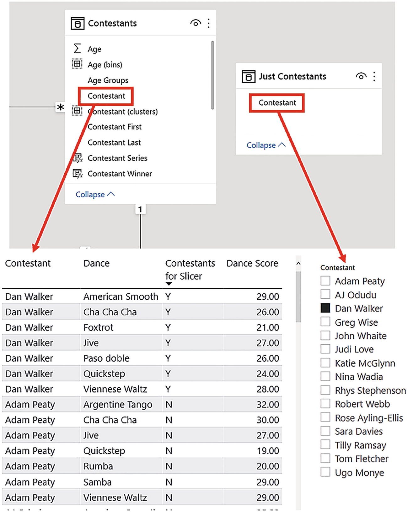
The column for the slicer comes from a different table

Next, I created a DAX measure, “Contestant for Slicer,” to flag up the selected value in the slicer:
Contestants for Slicer =
--Returns "Y" of the contestant has been selected in the slicer
    IF (
        SELECTEDVALUE ( 'Just Contestants'[Contestant] )
            = SELECTEDVALUE ( Contestants[Contestant] ),
                                                   "Y", "N")
I could then build the jitter plot visual which would require two plot segments, layered one on top of the other. The reason for the second plot segment is to show only the selected contestant’s data points, colored bright pink, so they sit on top of the gray data points; otherwise, the pink data points would lurk behind the gray ones. In PlotSegment1 (Figure 19-13), the Jitter sub-layout was applied with the “Dance” field bound to the x-axis and “Dance Score” bound to the y-axis. Although “Dance Score” is a numerical field, I changed it to categorical and therefore generated a second categorical axis. This plot segment used a gray filled symbol, each symbol representing 1 of 264 contestants.
Figure 19-13

The first plot segment used in the design of the jitter plot in Figure 19-11

The second plot segment is only used to show the values for the contestant selected in the slicer. This plot segment is a duplication of the first plot segment with the difference that the symbol is colored bright pink and the x- and y-axes have been hidden. To control the visibility of the symbol to only show the selected contestant’s data, I used the Visibility attribute of the symbol, binding the “Contestant for Slicer” measure and setting it to “Y”; see Figure 19-14.
Figure 19-14

The second plot segment shows the value for the contestant selected in the slicer

To finish the visual, I added text marks anchored to guides to label the x- and y-axes.

The downside of using the jitter plot is that the data points are arranged randomly in line with the scores on the y-axis, and therefore it’s difficult to see exactly where the clusters in the scores are gathered. An alternative way to visualize the contestants’ performance might be to use the Packing sub-layout rather than Jitter, and you can see the alternative version of the chart in Figure 19-15.
Figure 19-15

The Packing sub-layout is an alternative to the Jitter sub-layout

Which do you prefer? That’s one of the great benefits of using Charticulator; it’s so easy to render variations on a visual to get to the one that’s exactly right.

Arrow Chart

Let’s now consider a visualization that will make comparisons between two values selected in a slicer. In Figure 19-16, we are comparing salespeople’s sales between two years. In the top chart, the years are between 2019 and 2020, and in the bottom chart, between 2018 and 2019, the years being selected in the slicer. You can see that when comparing 2019 and 2020, sales were greater for all the salespeople in 2020, but comparing 2018 and 2019, sales in 2019 were less for salespeople “Charron” and “Reyer,” indicated by the reversed red arrow.
Figure 19-16

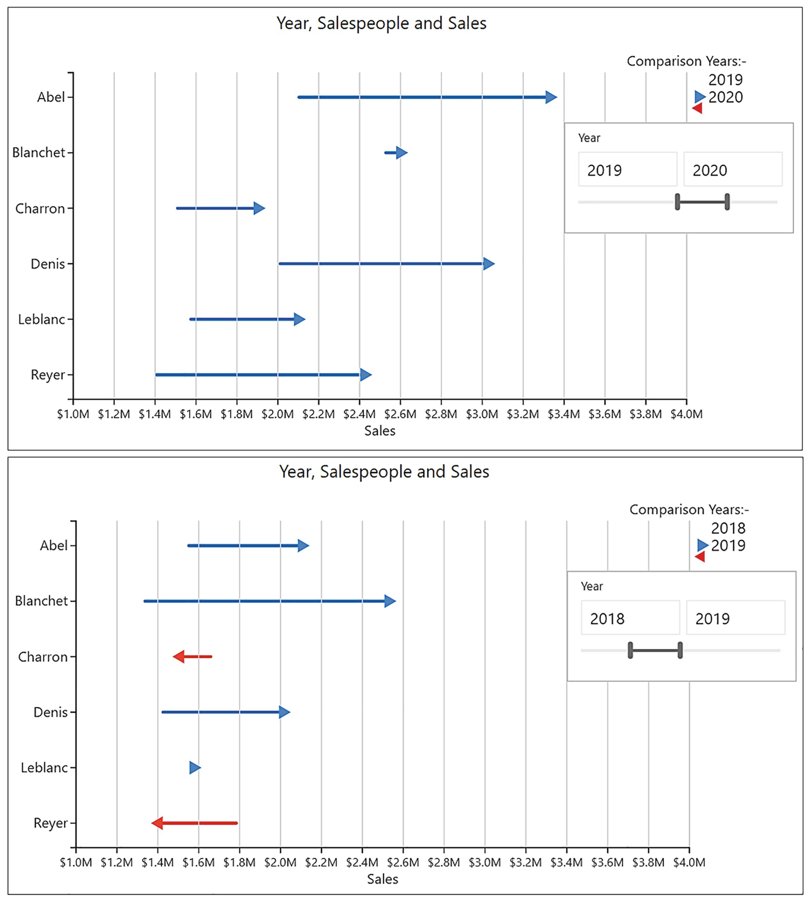
Arrow chart comparing yearly sales

The first consideration for this visual is to filter the sales so that only sales for the two years selected in the slicer show. For this, we used the following “Start or End” DAX measure:
Start or End =
VAR StartYr =
    MINX ( ALLSELECTED ( DateTable[Year] ), CALCULATE ( MIN (
                                         DateTable[Year] ) ) )
VAR EndYr =
    MAXX ( ALLSELECTED ( DateTable[Year] ), CALCULATE ( MAX (
                                        DateTable[Year] ) ) )
RETURN
    IF (
        SELECTEDVALUE ( DateTable[Year] ) = StartYr
            || SELECTEDVALUE ( DateTable[Year] ) = EndYr,
                                                 "Y", "N" )
You can see in Figure 19-17 how the measure evaluates when placed in a table visual.
Figure 19-17

The “Start or End” measure will be used to filter sales for the years selected in the slicer

When we create our Charticulator visual, we can put this measure into the visual level filter bucket in Power BI to filter out rows where the value is “Y” (Figure 19-18) and so only use the data for the selected years.
Figure 19-18

Using the visual level filter to filter years according to the slicer selection

To plot the arrows correctly on the chart according to the slicer selection, we can identify four rules:
  1. 1.

    Arrow symbols are only visible for the end year.

     
  2. 2.

    A blue arrow symbol is only visible when sales are greater in the end year.

     
  3. 3.

    A red arrow symbol is only visible when the sales are less in the end year.

     
  4. 4.

    The red arrow symbol must point in the opposite direction to the blue arrow symbol which will require two glyphs and therefore two plot segments.

     
This chart therefore makes extensive use of the Visibility attribute of the arrow symbol used in the Glyph pane to meet these rules, and we’ve used three DAX measures to provide the conditions whereby the arrow will be visible as follows (numbered for clarity):
1. Last Yr =
--Returns "Y" if the year is the end year.
IF (
    SELECTEDVALUE ( DateTable[Year] )
        = CALCULATE ( MAX ( DateTable[Year] ), ALLSELECTED (
                                            DateTable[year] ) ),
                                                      "Y",  "N")
2. Less Than =
--Returns "Y" if sales in the end year are less than sales in the start year.
VAR MinYr =
    CALCULATE ( MIN ( DateTable[Year] ), ALLSELECTED (
                                             DateTable[year] ) )
VAR MinSales =
    CALCULATE ( [Sales], DateTable[Year] = MinYr )
RETURN
    IF ( [Sales] > MinSales || [Sales] = MinSales, "N", "Y" )
3. Last and Not Less Than =
--Returns "Y" if sales are in the end year and sales are greater in the end year than in the start year.
IF ( [Last Yr] = "Y" && [Less Than] = "N", "Y", "N" )
We can see the results of these measures when placed in a table visual in Figure 19-19.
Figure 19-19

The three measures used to show or hide the arrows depending on the slicer selection

It would be nice if this were now the end of the DAX measures required by the visual. Unfortunately, the problem is that when we link the glyphs for each salesperson, in effect creating the arrow shaft, there is no Visibility attribute associated with a Link; we can only control the color of the line. Also, because the link line is associated with the first instance of the glyph, that is, for the start year, we need to color the line red if the sales in the start year are greater than the sales in the end year. Here is the DAX measure that will find these sales:
Less Than 2 =
--Returns "Y" if sales in the start year are greater than sales in the end year.
VAR MaxYr =
    CALCULATE ( MAX ( DateTable[Year] ), ALLSELECTED (
                                            DateTable[year] ) )
VAR MaxSales =
    CALCULATE ( [Sales], DateTable[Year] = MaxYr )
RETURN
    IF ( [Sales] < MaxSales || [Sales] = MaxSales, "N", "Y" )
You can see the evaluation of this measure when placed in a table visual in Figure 19-20.
Figure 19-20

The “Less Than 2” measure that is required for the link line

Table 19-1 clarifies the conditions that return the “Y” flag using the DAX measures.

Table 19-1. DAX measures and conditions that return “Y”

Measure Name

Returns “Y” if sales for …

Less Than

...End year  <  Start year

Last and Not Less Than

...End year  >  Start year

Less Than 2

...Start year  >  End year

At last, we are ready to build the arrow chart, and you can see the first plot segment required in Figure 19-21.
Figure 19-21

PlotSegment1 of the chart in Figure 19-16

You will see that “Sales” is bound to the x-axis, the Range attribute being edited to start at 1,000,000 and end at 4,000,000 (to account for values from any two years), and “Salespeople” bound to the y-axis. Gray gridlines have also been added.

A triangle symbol is used as the glyph, rotated to look like an arrowhead with a blue fill. The “Last and Not Less Than” measure has been bound to the Visibility attribute and set to “Y” (visible if sales in the end year are greater than sales in the start year).

The glyph is linked by Salespeople. The linking line takes its color from the start year, and so we need to bind the “Less Than 2” measure to the Link color and edit it so “Y” is red and “N” is blue (red if sales in the start year are greater than sales in the end year).

We are now ready to create the second plot segment that is required for the reverse pointing arrow; see Figure 19-22.
Figure 19-22

PlotSegment2 of the chart in Figure 19-16

This plot segment uses the same axes as PlotSegment1, but they are not visible. The glyph for this plot segment is a triangle, colored red and rotated accordingly. The “Less Than” measure is bound to the Visibility attribute of the arrow and set to “Y” (visible if sales in the end year are less than sales in the start year).

Finally, two additional plot segments were required to generate a “legend” which you can see in Figure 19-23.
Figure 19-23

PlotSegment3 and PlotSegment4 of the chart in Figure 19-16

In PlotSegment3, to generate the blue triangle beside the selected end year, it was necessary to group the plot segment by the “Year” field and then bind “Year” to the y-axis and move it to the opposite side. The triangle is a glyph with a blue Fill, and the Visibility is set to “Last and Not Less Than” = “Y.” To show a red triangle, a fourth plot segment was created in a similar way to PlotSegment3, but the triangle was given a red Fill, and the Visibility is set to “Last Yr” = “Y.”

The techniques that we’ve used to build this visual and indeed the other visuals that we’ve explored in this chapter can be used in many creative ways, so all that remains is for you to try them out for yourself.

This now brings us to the end of our journey through Charticulator. I hope you have been inspired by the numerous charts and visuals that you have learned to create along the way to build informative, persuasive, and interactive visuals that would not be possible to generate in Power BI or indeed with any other custom visual that you may have considered importing into Power BI.

Happy Charticulating!

..................Content has been hidden....................

You can't read the all page of ebook, please click here login for view all page.
Reset
18.224.37.68