Systems of Equations in Engineering |
CHAPTER 7 |
7.1 INTRODUCTION
The solution of a system of linear equations is an important topic for all engineering disciplines. In this chapter, the solution of 2 × 2 systems of equations will be carried out using four different methods: substitution method, graphical method, matrix algebra method, and Cramer's rule. It is assumed that the students are already familiar with the substitution and graphical methods from their high school algebra course, while the matrix algebra method and Cramer's rule are explained in detail. The objective of this chapter is to be able to solve the systems of equations encountered in beginning engineering courses such as physics, statics, dynamics, and DC circuit analysis. While the examples given are limited to 2 × 2 systems of equations, the matrix algebra approach is applicable to linear systems having any number of unknowns and is suitable for immediate implementation in MATLAB.
7.2 SOLUTION OF A TWO-LOOP CIRCUIT
Consider a two-loop resistive circuit with unknown currents I1 and I2 as shown in Fig. 7.1. Using a combination of Kirchhoff's voltage law (KVL) and Ohm's law, a system of two equations with two unknowns I1 and I2 can be obtained as
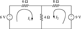
Figure 7.1 A two-loop resistive circuit.
Equations (7.1) and (7.2) represent a system of equations for I1 and I2 that can be solved using the four different methods outlined as follows:
-
Substitution Method: Solving equation (7.1) for the first variable I1 gives
The current I2 can now be solved by substituting I1 from equation (7.3) into equation (7.2), which gives
The current I1 can now be obtained by substituting the value of the second variable I2 from equation (7.4) into equation (7.3) as

Therefore, the solution of the system of equations (7.1) and (7.2) is given by
(I1, I2) = (0.3462 A, 0.6346 A).
-
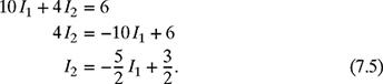
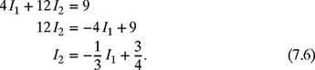
Graphical Method: Begin by assuming I1 as the independent variable and I2 as the dependent variable. Solving equation (7.1) for the dependent variable I2 gives
Similarly, solving equation (7.2) for I2 gives
Equations (7.5) and (7.6) are linear equations of the form y = mx + b. The simultaneous solution of equations (7.5) and (7.6) is the intersection point of the two lines. The plot of the two straight lines along with their intersection point is shown in Fig. 7.2. The intersection point, (I1, I2) ≈ (0.35A, 0.63A), is the solution of the 2 × 2 system of equations (7.1) and (7.2).
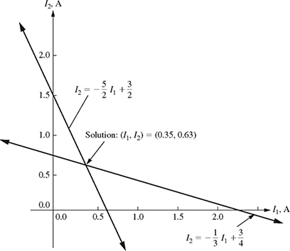
Figure 7.2 Plot of 2 × 2 system of equations (7.1) and (7.2).
Note that the graphical method gives only approximate results; therefore, this method is generally not used when an accurate result is needed. Also, if the two lines do not intersect, then one of the following two possibilities exist:
(i) The two lines are parallel lines (same slope but different y-intercepts) and the system of equations has no solution.
(ii) The two lines are parallel lines with same slope and y-intercept (the two lines lie on top of each other; they are the same line) and the system of equations has infinitely many solutions. In this case, the two equations are dependent (i.e., one equation can be obtained by performing linear operations on the other equation).
-
Matrix Algebra Method: The matrix algebra method can also be used to solve the system of equations given by equations (7.1) and (7.2). Rewriting the system of equations (7.1) and (7.2) in the form so that the two variables line up gives
Now, writing equations (7.7) and (7.8) in matrix form yields
Equation (7.9) is of the form Ax = b, where
is a 2 × 2 coefficient matrix,
is a 2 × 1 matrix (column vector) of unknowns, and
is a 2 × 1 matrix on the right-hand side (RHS) of equation (7.9) For any system of the form Ax = b, the solution is given by
x = A−1 b
where A−1 is the inverse of the matrix A. For a 2 × 2 system of equations where

the inverse of the matrix A is given by

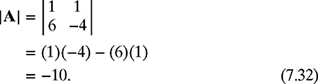
where Δ = ∣A∣ is the determinant of matrix A and is given by

Note that if Δ = ∣A∣ = 0, A−1 does not exist. In other words, the system of equations Ax = b has no solution. Now, for the two-loop circuit problem,

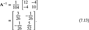
The inverse of matrix A is given by

where Δ = ∣A∣ = ad − cb = (10) (12) − (4) (4) = 104. Therefore, the inverse of matrix A can be calculated as
The solution of the system of equations
 can now be found by multiplying A−1 (given by equation (7.13)) with the column matrix b (given by equation (7.12)) as
The solution of the system of equations (7.1) and (7.2) is therefore given by
(I1, I2) = (0.3462A, 0.6346A).
-
Cramer's Rule: For any system Ax = b, the solution of the system of equations is given by
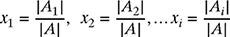
where ∣Ai∣ is obtained by replacing the ith column of the matrix A with the column vector b. Writing the 2 × 2 system of equations
a11 x1 + a12 x2 = b1
a21 x1 + a22 x2 = b2in matrix form as
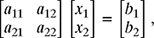
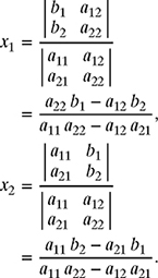
Cramer's rule gives the solution of the system of equations as
For the two-loop circuit, the 2 × 2 system of equations is

Using Cramer's rule, the currents I1 and I2 can be determined as
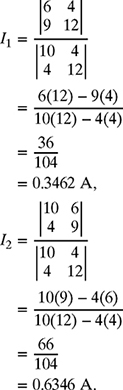
Therefore, I1 = 0.3462 A and I2 = 0.6346 A. Note that Cramer's rule is probably fastest for solving 2 × 2 systems but not faster than MATLAB.


7.3 TENSION IN CABLES
An object weighing 95 N is hanging from a roof with two cables as shown in Fig. 7.3. Determine the tension in each cable using the substitution, matrix algebra, and Cramer's rule methods.
Since the system shown in Fig. 7.3 is in equilibrium, the sum of all the forces shown in the free-body diagram must be equal to zero. This implies that all the forces in the x- and y-directions are equal to zero (see Chapter 4). The components of the tension ![]() in the x- and y-directions are given by −T1 cos(45°) N and T1 sin(45°) N, respectively. Similarly, the components of the tension
in the x- and y-directions are given by −T1 cos(45°) N and T1 sin(45°) N, respectively. Similarly, the components of the tension ![]() in the x- and y-directions are given by T2 cos(30°) N and T2 sin(30°) N, respectively. The components of the object weight is 0 N in the x-direction and −95 N in the y-direction. Summing all the forces in the x-direction gives
in the x- and y-directions are given by T2 cos(30°) N and T2 sin(30°) N, respectively. The components of the object weight is 0 N in the x-direction and −95 N in the y-direction. Summing all the forces in the x-direction gives

Figure 7.3 A 95 N object hanging from two cables.
Similarly, summing the forces in the y-direction yields
Equations (7.14) and (7.15) make a 2 × 2 system of equations with two unknowns T1 and T2 that can be written in matrix form as
The solution of the system of equations (T1 and T2) will now be obtained using three methods: the substitution method, the matrix algebra method, and Cramer's rule.
-
Substitution Method: Using equation (7.14), the second variable T2 is found in terms of the first variable T1 as
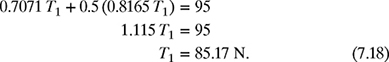
Substituting T2 from equation (7.17) into equation (7.15) gives
Now, substituting T1 obtained in equation (7.18) into equation (7.17) yields
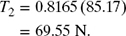
Therefore, T1 = 85.2 N and T2 = 69.6 N.
-
Matrix Algebra Method: The two unknowns (T1 and T2) in the 2 × 2 system of equations (7.14) and (7.15) are now determined using the matrix algebra method. Write equations (7.14) and (7.15) in the matrix form as
where matrices A, x, and b are given by
Therefore, the solution of the 2 × 2 system of equations
 can be found by solving equation (7.19) as
where A−1 is the inverse of matrix A. If A
 , then
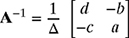
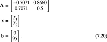
where Δ = ad − bc. Since, for this example, a = −0.7071, b = 0.8660, c = 0.7071, and d = 0.5, therefore,
Substituting matrices A−1 from equation (7.22) and b from equation (7.20) into equation (7.21) gives
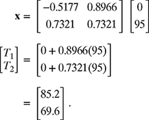
Therefore, T1 = 85.2 N and T2 = 69.6 N.
-
Cramer's Rule: The two unknowns (T1 and T2) in the 2 × 2 system of equations (7.14) and (7.15) are now determined using Cramer's rule. Using matrix equation (7.19), the tensions T1 and T2 can be found as

Therefore, T1 = 85.2 N and T2 = 69.6 N.

7.4 FURTHER EXAMPLES OF SYSTEMS OF EQUATIONS IN ENGINEERING
Reaction Forces on a Vehicle: The weight of a vehicle is supported by reaction forces at its front and rear wheels as shown in Fig. 7.4. If the weight is W = 4800 lb, the reaction forces R1 and R2 satisfy the equation:
Also, suppose that
(a) Find R1 and R2 using the substitution method.
(b) Write the system of equations (7.23) and (7.24) in the matrix form Ax = b, where ![]() .
.
(c) Find R1 and R2 using the matrix algebra method. Perform all computations by hand and show all steps.
(d) Find R1 and R2 using Cramer's rule.

Solution
(a) Substitution Method: Using equation (7.23), find R1 in terms of R2 as
Substituting R1 from equation (7.25) into equation (7.24) gives

Now, substituting R2 from equation (7.26) into equation (7.25) yields
![]()
Therefore, R1 = 1920 lb and R2 =; 2880 lb.
(b) Writing equations (7.23) and (7.24) in the matrix form gives
(c) Matrix Algebra Method: From the matrix equation (7.27), the matrices A, x, and b are given by
The reaction forces can be found by finding the inverse of matrix A and then multiplying this with column matrix b as
x = A−1 b
where
and
Substituting equation (7.32) in equation (7.31), the inverse of matrix A is given by

The reaction forces can now be found by multiplying A−1 in equation (7.33) with matrix b given in equation (7.29) as
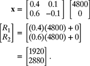
Therefore, R1 = 1920 lb and R2 = 2880 lb.
(d) Cramer's Rule: The reaction forces R1 and R2 can be found by solving the system of equations (7.23) and (7.24) using Cramer's rule as

Therefore, R1 = 1920 lb and R2 = 2880 lb.
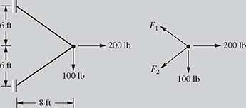
External Forces Acting on a Truss: A two-bar truss is subjected to external forces in both the horizontal and vertical directions as shown in Fig. 7.5. The forces F1 and F2 satisfy the following system of equations:
(a) Find F1 and F2 using the substitution method.
(b) Write the system of equations (7.34) and (7.35) in the matrix form Ax = b, where ![]() .
.
(c) Find F1 and F2 using the matrix algebra method. Perform all computations by hand and show all steps.
(d) Find F1 and F2 using Cramer's rule.
(a) Substitution Method: Using equation (7.34), find force F1 in terms of F2 as
Substituting F1 from equation (7.36) into equation (7.35) gives
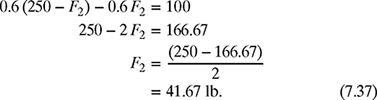
Now, substituting F2 from equation (7.37) into equation (7.36) yields
![]()
Therefore, F1 = 208.33 lb and F2 = 41.67 lb.
(b) Writing equations (7.34) and (7.35) in the matrix form yields
(c) Matrix Algebra Method: Writing matrix equation in (7.38) in the form Ax = b gives
The forces F1 and F2 can be found by finding the inverse of matrix A and then multiplying this with matrix b as
x = A−1 b
where
and

Substituting equation (7.43) in equation (7.42), the inverse of matrix A is given by
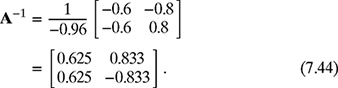
The forces F1 and F2 can now be found by multiplying A−1 in equation (7.44) by column matrix b given in equation (7.40) as

Therefore, F1 = 208.33 lb and F2 = 41.67 lb.
(d) Cramer's Rule: The forces F1 and F2 can be found by solving the system of equations (7.34) and (7.35) using Cramer's rule as

Therefore, F1 = 208.33 lb and R2 = 41.67 lb.
Summing Op-Amp Circuit: A summing Op-Amp circuit is shown in Fig. 7.6. An analysis of the Op-Amp circuit shows that the conductances G1 and G2 in mho (℧) satisfy the following system of equations:
(a) Find G1 and G2 using the substitution method.
(b) Write the system of equations (7.45) and (7.46) in the matrix form Ax = b, where ![]() .
.
(c) Find G1 and G2 using the matrix algebra method. Perform all computations by hand and show all steps.
(d) Find G1 and G2 using Cramer's rule.

Solution
(a) Substitution Method: Using equation (7.45), find the admittance G1 in terms of G2 as
Substituting G1 from equation (7.47) into equation (7.46) gives
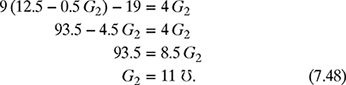
Now, substituting G2 from equation (7.48) into equation (7.47) yields
![]()
Therefore, G1 = 7 ℧ and G2 = 11 ℧.
(b) Rewrite equations (7.45) and (7.46) in the form
Now, write equations (7.49) and (7.50) in matrix form as
(c) Matrix Algebra Method: Writing the matrix equation in (7.64) in the form Ax = b gives
The admittance G1 and G2 can be found by finding the inverse of matrix A and then multiplying this with matrix b as
x = A−1 b
where
and

Substituting equation (7.56) in equation (7.55), the inverse of matrix A is given as
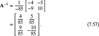
The admittance G1 and G2 can now be found by multiplying A−1 in equation (7.57) and the column matrix b given in equation (7.53) as
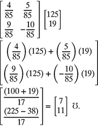
Therefore, G1 = 7 ℧ and G2 =11 ℧.
(d) Cramer's Rule: The admittance G1 and G2 can be found by solving the system of equations (7.45) and (7.46) using Cramer's rule as

Therefore, G1 = 7 ℧ and G2 =11 ℧.
Force on the Gastrocnemius Muscle: A driver applies a steady force of FP = 30 N against a gas pedal, as shown in Fig. 7.7. The free-body diagram of the driver's foot is also shown. Based on the x-y coordinate system shown, the force of the gastrocnemius muscle Fm and the weight of the foot WF satisfy the following system of equations:
where Rx and Ry are the reactions at the ankle.
(a) Suppose ![]() N and Ry = 120 N. Write the system of equations in terms of Fm and WF.
N and Ry = 120 N. Write the system of equations in terms of Fm and WF.
(b) Find Fm and WF using the substitution method.
(c) Write the system of equations (7.58) and (7.59) in the matrix form Ax = b, where ![]() .
.
(d) Find Fm and WF using the matrix algebra method. Perform all computations by hand and show all steps.
(e) Find Fm and WF using Cramer's rule.

Figure 7.7 A driver applying a steady force against the gas pedal.
Solution
(a) Rewriting equations (7.58) and (7.59) in terms of given information yields
(b) Substitution Method: Using equation (7.60), find the force Fm in terms of WF as
Substituting Fm from equation (7.62) into equation (7.61) gives
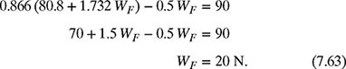
Now, substituting WF from equation (7.63) into equation (7.62) yields
![]()
Therefore, Fm = 115.4 N and WF = 20 N.
(c) Writing equations (7.60) and (7.61) in the matrix form Ax = b gives

(d) Matrix Algebra Method: The forces Fm and WF can be found by finding the inverse of the matrix A and then multiplying this by vector b as
x = A−1 b,
where
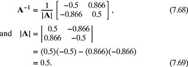
Substituting equation (7.69) in equation (7.68), the inverse of matrix A is given as

The forces Fm and WF can now be found by multiplying A−1 in equation (7.70) and the column matrix b given in equation (7.66) as
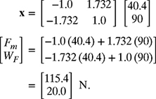
Therefore, Fm = 115.4 N and WF = 20 N.
(e) Cramer's Rule: The forces Fm and WF can be found by solving the system of equations (7.60) and (7.61) using Cramer's rule as

Therefore, Fm = 115.4 N and WF = 20 N.
Two-Component Blending of Liquids: An environmental engineer wishes to blend a single mixture of insecticide spray solution of volume V = 1000 L and concentration C = 0.15 from two spray solutions of concentrations c1 = 0.12 and c2 = 0.17. The required volumes of the two spray solutions v1 and v2 can be determined from a system of equations describing conditions for volume and concentration, respectively, as
(a) Knowing that V = 1000 L, c1 = 0.12, c2 = 0.17, and C = 0.15, rewrite the system of equations in terms of v1 and v2.
(b) Find v1 and v2 using the substitution method.
(c) Write the system of equations (7.71) and (7.72) in the matrix form Ax = b, where ![]() .
.
(d) Find v1 and v2 using the matrix algebra method. Perform all computations by hand and show all steps.
(e) Find v1 and v2 using Cramer's rule.
Solution
(a) Rewriting equations (7.71) and (7.72) in terms of the given information yields
(b) Substitution Method: Using equation (7.73), find the volume v2 in terms of v1 as
Substituting v2 from equation (7.75) into equation (7.74) gives

Now, substituting v1 from equation (7.76) into equation (7.75) yields
![]()
Therefore, v1 = 400 L and v2 = 600 L.
(c) Writing equations (7.73) and (7.74) in matrix form Ax = b gives
where
(d) Matrix Algebra Method: The volumes v1 and v2 can be found by finding the inverse of the matrix A and then multiplying this by column vector b as
x = A−1 b,
where

Substituting equation (7.82) in equation (7.81), the inverse of matrix A is given as

The volumes v1 and v2 can now be found by multiplying A−1 in equation (7.83) and the column vector b given in equation (7.79) as
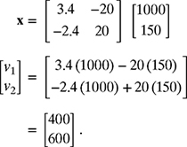
Therefore, v1= 400 L and v2 = 600 L.
(e) Cramer's Rule: The volumes v1 and v2 can be found by solving the system of equations (7.73) and (7.74) using Cramer's rule as

Therefore, v1 = 400 L and v2 = 600 L.
PROBLEMS
-
7-1. Consider the two-loop circuit shown in Fig. P7.1. The currents I1 and I2 (in A) satisfy the following system of equations:
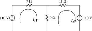
Figure P7.1 Two-loop circuit for problem P7-1.
(a) Find I1 and I2 using the substitution method.
(b) Write the system of equations (7.84) and (7.85) in the matrix form AI = b, where I =
 .
.(c) Find I1 and I2 using the matrix algebra method. Perform all computations by hand and show all steps.
(d) Find I1 and I2 using Cramer's rule.
-
7-2. Consider the two-loop circuit shown in Fig. P7.2. The currents I1 and I2 (in A) satisfy the following system of equations:
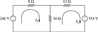
Figure P7.2 Two-loop circuit for problem P7-2.
(a) Find I1 and I2 using the substitution method.
(b) Write the system of equations (7.86) and (7.87) in the matrix form AI = b, where
 .
.(c) Find I1 and I2 using the matrix algebra method. Perform all computations by hand and show all steps.
(d) Find I1 and I2 using Cramer's rule.
-
7-3. Consider the two-loop circuit shown in Fig. P7.3. The currents I1 and I2 (in A) satisfy the following system of equations:
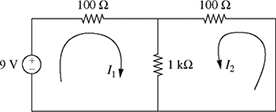
Figure P7.3 Two-loop circuit for problem P7-3.
(a) Find I1 and I2 using the substitution method.
(b) Write the system of equations (7.88) and (7.89) in the matrix form AI = b, where
 .
.(c) Find I1 and I2 using the matrix algebra method. Perform all computations by hand and show all steps.
(d) Find I1 and I2 using Cramer's rule.
-
7-4. Consider the two-node circuit shown in Fig. P7.4. The voltages V1 and V2 (in V) satisfy the following system of equations:
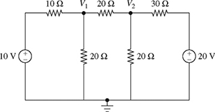
Figure P7.4 Two-node circuit for problem P7-4.
(a) Find V1 and V2 using the substitution method.
(b) Write the system of equations (7.90) and (7.91) in the matrix form AV = b, where
 .
.(c) Find V1 and V2 using the matrix algebra method. Perform all computations by hand and show all steps.
(d) Find V1 and V2 using Cramer's rule.
-
7-5. Consider the two-node circuit shown in Fig. P7.5. The voltages V1 and V2 (in V) satisfy the following system of equations:
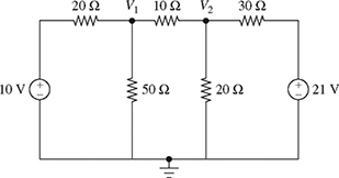
Figure P7.5 Two-node circuit for problem P7-5.
(a) Find V1 and V2 using the substitution method.
(b) Write the system of equations (7.92) and (7.93) in the matrix form AV = b, where
.(c) Find V1 and V2 using the matrix algebra method. Perform all computations by hand and show all steps.
(d) Find V1 and V2 using Cramer's rule.
-
7-6. Consider the two-node circuit shown in Fig. P7.6. The voltages V1 and V2 (in V) satisfy the following system of equations:
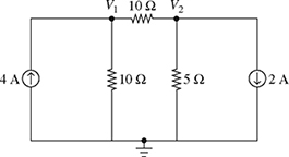
Figure P7.6 Two-node circuit for problem P7-6.
(a) Find V1 and V2 using the substitution method.
(b) Write the system of equations (7.94) and (7.95) in the matrix form AV = b, where
 .
.(c) Find V1 and V2 using the matrix algebra method. Perform all computations by hand and show all steps.
(d) Find V1 and V2 using Cramer's rule.
-
7-7. An analysis of the circuit shown in Fig. P7.7 yields the following system of equations:

Figure P7.7 Two-node circuit for problem P7-7.
(a) Find V1 and V2 using the substitution method.
(b) Write the system of equations (7.96) and (7.97) in the matrix form AV = b, where
.(c) Find V1 and V2 using the matrix algebra method. Perform all computations by hand and show all steps.
(d) Find V1 and V2 using Cramer's rule.
-
7-8. A summing Op-Amp circuit is shown in Fig. 7.6. An analysis of the Op-Amp circuit shows that the admittances G1 and G2 in mho (℧) satisfy the following system of equations:
(a) Find G1 and G2 using the substitution method.
(b) Write the system of equations (7.98) and (7.99) in the matrix form AG = b, where
 .
.(c) Find G1 and G2 using the matrix algebra method. Perform all computations by hand and show all steps.
(d) Find G1 and G2 using Cramer's rule.
-
7-9. A summing Op-Amp circuit is shown in Fig. 7.6. An analysis of the Op-Amp circuit shows that the admittances G1 and G2 in mho (℧) satisfy the following system of equations:
(a) Find G1 and G2 using the substitution method.
(b) Write the system of equations (7.100) and (7.101) in the matrix form AG = b, where
.(c) Find G1 and G2 using the matrix algebra method. Perform all computations by hand and show all steps.
(d) Find G1 and G2 using Cramer's rule.
-
7-10. A 20 kg object is suspended by two cables as shown in Fig. P7.10. The tensions T1 and T2 satisfy the following system of equations:
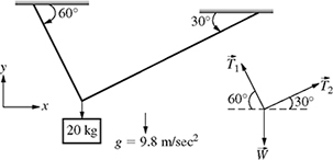
Figure P7.10 A 20 kg object suspended by two cables for problem P7-10.
(a) Write the system of equations (7.100) and (7.101) in the matrix form AT = b, where

In other words, find matrices A and b. What are the dimensions of A and b?
(b) Find T1 and T2 using the matrix algebra method. Perform all matrix computation by hand.
(c) Find T1 and T2 using Cramer's rule.
-
7-11. A 100 lb weight is suspended by two cables as shown in Fig. P7.11. The tensions T1 and T2 satisfy the following system of equations:
(a) Write the system of equations (7.104) and (7.105) in the matrix form Ax = b, where

In other words, find matrices A and b.
(b) Find T1 and T2 using the matrix algebra method. Perform all matrix computation by hand and show all steps.
(c) Find T1 and T2 using Cramer's rule.
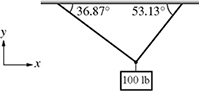

Figure P7.11 A 100 lb weight suspended by two cables for problem P7-11.
-
7-12. A two-bar truss supports a weight of W = 750 lb as shown in Fig. P7.12. The forces F1 and F2 satisfy the following system of equations:
(a) Write the system of equations (7.106) and (7.107) in the matrix form AF = b, where

In other words, find matrices A and b.
(b) Find F1 and F2 using the matrix algebra method. Perform all matrix computation by hand and show all steps.
(c) Find F1 and F2 using Cramer's rule.


Figure P7.12 A two-bar truss supporting a weight for problem P7-12.
-
7-13. A 10 kg object is suspended from a two-bar truss shown in Fig. P7.13. The forces F1 and F2 satisfy the following system of equations:


Figure P7.13 An object suspended from a two-bar truss for problem P7-13.
(a) Write the system of equations (7.108) and (7.109) in the matrix form AF = b, where

In other words, find matrices A and b.
(b) Find F1 and F2 using the matrix algebra method. Perform all matrix computation by hand and show all steps.
(c) Find F1 and F2 using Cramer's rule.
-
7-14. A F = 100 N force is applied to a two-bar truss as shown in Fig. P7.14. The forces F1 and F2 satisfy the following system of equations:
(a) Write the system of equations (7.110) and (7.111) in the matrix form AF = b, where

In other words, find matrices A and b.
(b) Find F1 and F2 using the matrix algebra method. Perform all matrix computation by hand and show all steps.
(c) Find F1 and F2 using Cramer's rule.


Figure P7.14 A 100 N force applied to a two-bar truss for problem P7-14.
-
7-15. A force F = 200 lb is applied to a two-bar truss as shown in Fig. P7.15. The forces F1 and F2 satisfy the following system of equations:
(a) Write the system of equations (7.112) and (7.113) in the matrix form AF = b, where
In other words, find matrices A and b.
(b) Find F1 and F2 using the matrix algebra method. Perform all matrix computation by hand and show all steps.
(c) Find F1 and F2 using Cramer's rule.

Figure P7.15 A 200 lb force applied to a two-bar truss for problem P7-15.
-
7-16. The weight of a vehicle is supported by reaction forces at its front and rear wheels as shown in Fig. P7.16. If the weight of the vehicle is W = 4800 lb, the reaction forces R1 and R2 satisfy the following system of equations:
(a) Find R1 and R2 using the substitution method.
(b) Write the system of equations (7.114) and (7.115) in the matrix form Ax = b, where

In other words, find matrices A and b.
(c) Find R1 and R2 using the matrix algebra method. Perform all matrix computation by hand and show all steps.
(d) Find R1 and R2 using Cramer's rule.

-
7-17. Solve problem P7-16 if the system of equations are given by equations (7.116) and (7.117).
-
7-18. Solve problem P7-16 if the system of equations are given by (7.118) and (7.119).
-
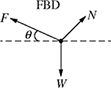
7-19. A vehicle weighing W = 10 kN is parked on an inclined driveway (θ = 21.8°) as shown in Fig. P7.19. The forces F and N satisfy the following system of equations:
where forces F and N are in kN.
(a) Write the system of equations (7.120) and (7.121). in the matrix form Ax = b, where

In other words, find matrices A and b.
(b) Find F and N using the matrix algebra method. Perform all matrix computations by hand and show all steps.
(c) Find F and N using Cramer's rule.

-
7-20. A vehicle weighing W = 2000 lb is parked on an inclined driveway (θ = 35°) as shown in Fig. P7.19. The forces F and N satisfy the following system of equations:
where forces F and N are in lb. Solve parts (a)–(c) of problem P7-19 for system of equations given by (7.122) and (7.123).
-
7-21. A 100 lb crate weighing W = 100 lb is pushed against an incline (θ = 30°) with a force of Fa = 30 lb as shown in Fig. P7.21. The forces Ff and N satisfy the following system of equations:
(a) Write the system of equations (7.124) and (7.125) in the matrix form Ax = b, where

In other words, find matrices A and b.
(b) Find Ff and N using the matrix algebra method. Perform all matrix computation by hand and show all steps.
(c) Find Ff and N using Cramer's rule.

-
7-22. A crate weighing W = 500 N is pushed against an incline (θ = 20°) with a force of Fa = 100 N as shown in Fig. P7.21. The forces Ff and N satisfy the following system of equations:
Solve parts (a)–(c) of problem P7-21 for system of equations given by (7.126) and (7.127).
-
7-23. A 100 kg desk rests on a horizontal plane with a coefficient of friction of μ = 0.4. It is pulled with a force of F = 800 N at an angle of θ = 45° as shown in Fig. P7.23. The normal force Nf and acceleration a in m/s2 satisfy the following system of equations:
(a) Find Nf and a using the substitution method.
(b) Write the system of equations (7.128) and (7.129) in the matrix form Ax = b, where

In other words, find matrices A and b.
(c) Find Nf and a using the matrix algebra method.
(d) Find Nf and a using Cramer's rule.

-
7-24. A 200 kg desk rests on a horizontal plane with a coefficient of friction of μ = 0.3. It is pulled with a force of F = 1000 N at an angle of θ = 20° as shown in Fig. P7.23. The normal force Nf and acceleration a in m/s2 satisfy the following system of equations:
Solve parts (a)–(d) of problem P7-23 for system of equations (7.130) and (7.131).
-
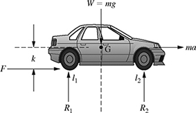
7-25. The weight of a vehicle is supported by reaction forces at its front and rear wheels as shown in Fig. P7.25. The reaction forces R1 and R2 satisfy the following system of equations:
(a) Write the system of equations (7.132) and (7.133) if l1 = 2 m, l2 = 1.5 m, k = 1.5 m, g = 9.81 m/s2, m = 1000 kg, and a = 5 m/s2.
(b) For the system of equations found in part (a), find R1 and R2 using the substitution method.
(c) Write the system of equations in the matrix form Ax = b, where

In other words, find matrices A and b.
(d) Find R1 and R2 using the matrix algebra method.
(e) Find R1 and R2 using Cramer's rule.
-
7-26. Repeat problem P7-25, if l1 = 2 m, l2 = 1.5 m, k = 1.5 m, g = 9.81 m/s2, m = 1000 kg, and a = −5 m/s2.
-
7-27. Repeat problem P7-25, if l1 = 2 m, l2 = 2 m, k = 1.5 m, g = 9.81 m/s2, m = 1200 kg, and a = 4.5 m/s2.
-
7-28. Repeat problem P7-25, if l1 = 2 m, l2 = 2 m, k = 1.5 m, g = 9.81 m/s2, m = 1200 kg, and a = −4.5 m/s2.
-
7-29. A driver applies a steady force of FP = 25 N against a gas pedal, as shown in Fig. P7.29. The free-body diagram of the driver's foot is also shown. Based on the x-y coordinate system shown, the force of the gastrocnemius muscle Fm and the weight of the foot WF satisfy the following system of equations:

Figure P7.29 A driver applying a steady force against the gas pedal.
(a) Knowing that
 N and Ry = 105 N, rewrite the system of equations (7.134) and (7.135) in terms of Fm and WF.
(b) Find Fm and WF using the substitution method.
(c) Write the system of equations obtained in part (a) in the matrix form Ax = b, where
 .
.(d) Find Fm and WF using the matrix algebra method. Perform all computations by hand and show all steps.
(e) Find Fm and WF using Cramer's rule.
-
7-30. An environmental engineer wishes to blend a single mixture of insecticide spray solution of volume V = 500 L with a specified concentration C = 0.2 from two spray solutions of concentration c1 = 0.15 and c2 = 0.25. The required volumes of the two spray solutions v1 and v2 can be determined from a system of equations describing conditions for volume and concentration, respectively as
(a) Knowing that V = 500 L, c1 = 0.15, c2 = 0.25, and C = 0.2, rewrite the system of equations (7.136) and (7.137) in terms of v1 and v2.
(b) Find v1 and v2 using the substitution method.
(c) Write the system of equations obtained in part (a) in the matrix form Ax = b, where
 .
.(d) Find v1 and v2 using the matrix algebra method. Perform all computations by hand and show all steps.
(e) Find v1 and v2 using Cramer's rule.
-
7-31. Repeat problem P7-30 if V = 400 L, C = 0.25, c1 = 0.2, and c2 = 0.4.
-
7-32. Consider the two-loop circuit shown in Fig. P7.32. The currents I1 and I2 (in A) satisfy the following system of equations:
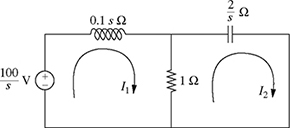
Figure P7.32 Two-loop circuit for problem P7-32.
(a) Find I1 and I2 using the substitution method.
(b) Write the system of equations (7.138) and (7.139) in the matrix form AI = b, where
.(c) Find I1 and I2 using the matrix algebra method.
(d) Find I1 and I2 using Cramer's rule.
-
7-33. Consider the two-loop circuit shown in Fig. P7.33. The currents I1 and I2 (in A) satisfy the following system of equations:

Figure P7.33 Two-loop circuit for problem P7-33.
(a) Find I1 and I2 using the the substitution method.
(b) Write the system of equations (7.140) and (7.141) in the matrix form AI = b, where
.(c) Find I1 and I2 using the matrix algebra method.
(d) Find I1 and I2 using Cramer's rule.
-
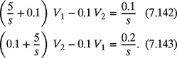
7-34. Consider the two-node circuit shown in Fig. P7.34. The voltages V1 and V2 (in V) satisfy the following system of equations:

Figure P7.34 Two-loop circuit for problem P7-34.
(a) Write the system of equations (7.142) and (7.143) in the matrix form AV = b, where
 .
.(b) Find V1 and V2 using the matrix algebra method.
(c) Find V1 and V2 using Cramer's rule.
-
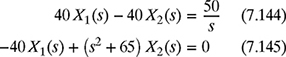
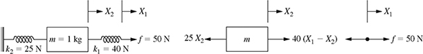
7-35. A mechanical system along with its free body diagram is shown in Fig. P7.35, where f = 50 N is the applied force. The linear displacements X1(s) and X2(s) of the two springs in the s-domain satisfy the following system of equations:
(a) Write the system of equations (7.144) and (7.145) in the matrix form AX(s) = b, where X(s) =
 .
.(b) Find the expressions of X1(s) and X2(s) using the matrix algebra method.
(c) Find the expressions of X1(s) and X2(s) using Cramer's rule.
-
7-36. Fig. P7.36 shows a system with two-mass elements and two springs. The mass m1 is pulled with a force f = 100 N, and the displacements X1(s) and X2(s) of the two masses in the s-domain satisfy the following system of equations:
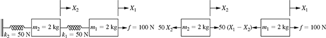
Figure P7.36 Mechanical system for problem P7-36.
(a) Write the system of equations (7.146) and (7.146) in the matrix form AX(s) = b, where X(s) =
 .
.(b) Find the expressions of X1(s) and X2(s) using the matrix algebra method.
(c) Find the expressions of X1(s) and X2(s) using Cramer's rule.
-
7-37. A co-op student at a composite materials manufacturing company is attempting to determine how much of two different composite materials to make from the available quantities of carbon fiber and resin. The student knows that Composite A requires 0.15 pounds of carbon fiber and 1.6 ounces of polymer resin while Composite B requires 3.2 pounds of carbon fiber and 2.0 ounces of polymer resin. If the available quantities of carbon fiber and resin are 15 pounds and 10 ounces, respectively, the amount of each composite to manufacture satisfies the system of equations:
where xA and xB are the amounts of Composite A and B (in pounds), respectively.
(a) Find xA and xB using the substitution method.
(b) Write the system of equations (7.148) and (7.149) in the matrix form Ax = b, where
 .
.(c) Find xA and xB using the matrix algebra method. Perform computation by hand and show all steps.
(d) Find xA and xB using Cramer's rule.
-
7-38. Repeat parts (a)–(d) of problem P7-37 if Composite A requires 1.6 pounds of carbon fiber and 0.5 ounces of polymer resin while Composite B requires 1.75 pounds of carbon fiber and 0.78 ounces of polymer resin. If the available quantities of carbon fiber and resin are 17 pounds and 12 ounces, respectively, the amount of each composite to manufacture satisfies the system of equations (7.150) and (7.151).
-
7-39. A structural engineer is performing a finite element analysis on an aluminum truss support structure subjected to a load as shown in Fig. P7.39. By the finite element method, the displacements in the horizontal and vertical directions at the node where the load is applied can be determined from the system of equations:
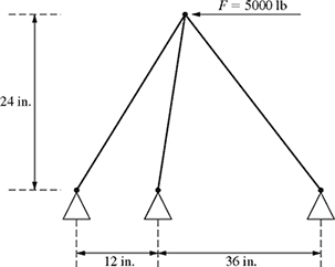
Figure P7.39 Finite element idealization of truss structure subject to loading.
where u and v are the the displacements in the horizontal and vertical directions, respectively.
(a) Find u and v using the substitution method.
(b) Write the system of equations (7.152) and (7.153) in the matrix form Ax = b, where
 .
.(c) Find u and v using the matrix algebra method. Perform computation by hand and show all steps.
(d) Find u and v using Cramer's rule.
-
7-40. A structural engineer is designing a crane that is to be used to unload barges at a dock. She is using a technique called finite element analysis to determine the displacement at the end of the crane. The finite element idealization of the crane structure picking up a 2000 lb load is shown in Fig. P7.40. The displacement in the horizontal and vertical directions at the end of the crane can be determined from the system of equations:
where u and v are the the displacements in the horizontal and vertical directions, respectively.
(a) Find u and v using the substitution method.
(b) Write the system of equations (7.154) and (7.155) in the matrix form Ax = b, where
.(c) Find u and v using the matrix algebra method. Perform computation by hand and show all steps.
(d) Find u and v using Cramer's rule.

Figure P7.40 Finite element idealization of crane structure subject to loading.