Derivatives in Engineering |
CHAPTER 8 |
8.1 INTRODUCTION
This chapter will discuss what a derivative is and why it is important in engineering. The concepts of maxima and minima along with the applications of derivatives to solve engineering problems in dynamics, electric circuits, and mechanics of materials are emphasized.
8.1.1 What Is a Derivative?
To explain what a derivative is, an engineering professor asks a student to drop a ball (shown in Fig. 8.1) from a height of y = 1.0 m to find the time when it impacts the ground. Using a high-resolution stopwatch, the student measures the time at impact as t = 0.452 s. The professor then poses the following questions:
(a) What is the average velocity of the ball?
(b) What is the speed of the ball at impact?
(c) How fast is the ball accelerating?

Figure 8.1 A ball dropped from a height of 1 meter.
Using the given information, the student provides the following answers:
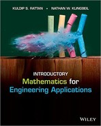
(a) Average Velocity, ![]() : The average velocity is the total distance traveled per unit time, i.e.,
: The average velocity is the total distance traveled per unit time, i.e.,
Note that the negative sign means the ball is moving in the negative y-direction.
(b) Speed at Impact: The student finds that there is not enough information to find the speed of ball when it impacts the ground. Using an ultrasonic motion detector in the laboratory, the student repeats the experiment and collects the data given in Table 8.1.
TABLE 8.1 Additional data collected from the dropped ball.

The student then calculates the average velocity ![]() in each interval. For example, in the interval t = [0, 0.1],
in each interval. For example, in the interval t = [0, 0.1], ![]() . The average velocity in the remaining intervals is given in Table 8.2.
. The average velocity in the remaining intervals is given in Table 8.2.
TABLE 8.2 Average velocity of the ball in different intervals

The student proposes an approximate answer of −4.13 m/s as the speed of impact with ground, but claims that he/she would need an infinite (∞) number of data points to get it exactly right, i.e.,
![]()
The professor suggests that this looks like the definition of a derivative, i.e.,
![]()
where, Δt = 0.452 − t.
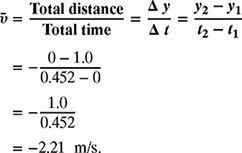
The derivatives of some common functions in engineering are given below. Note that ω, a, n, c, c1, and c2 are constants and not functions of t.
TABLE 8.3 Some common derivatives used in engineering.
The professor then suggests a quadratic curve fit of the measured data, which gives
y(t) = 1.0 − 4.905 t2.
The velocity at any time is thus calculated by taking the derivative as

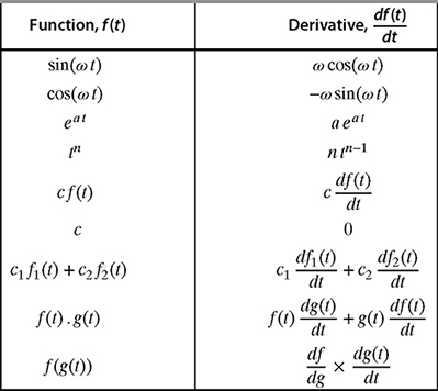
(c) The student is now asked to find the acceleration without taking any more data. The acceleration is the rate of change of velocity, i.e.,
Thus, if v(t) = −9.81 t, then

Hence, the acceleration due to gravity is constant and is equal to −9.81 m/s2.
8.2 MAXIMA AND MINIMA
Suppose now that the ball is thrown upward with an initial velocity vo = 4.43 m/s as shown in Fig. 8.2.
(a) How long does it take for the ball to reach its maximum height?
(b) What is the velocity at y = ymax?
(c) What is the maximum height ymax achieved by the ball?
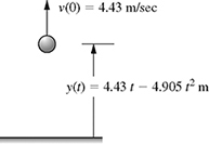
Figure 8.2 A ball thrown upward.
The professor suggests that the height of the ball is governed by the quadratic equation
and plotted as shown in Fig. 8.3.

Figure 8.3 The height of the ball thrown upward.
Based on the definition of the derivative, the velocity v(t) at any time t is the slope of the line tangent to y(t) at that instant, as shown in Fig. 8.4. Therefore, at the time when y = ymax, the slope of the tangent line is zero (Fig. 8.5).

Figure 8.4 The derivative as the slope of the tangent line.
For the problem at hand, the velocity is given by


Figure 8.5 The slope of the tangent line at maximum height.
Given equation (8.2), the student answers the professor's questions as follows:
(a) How long does it take to reach maximum height? At the time of maximum height t = tmax, ![]() . Hence, setting v(t) in equation (8.2) to zero gives
. Hence, setting v(t) in equation (8.2) to zero gives

or
tmax = 0.4515 s.
Therefore, it takes 0.4515 s for the ball to reach the maximum height.
(b) What is the velocity at y = ymax? Since the slope of the height at t = tmax is zero, the velocity at y = ymax is zero. The plot of the velocity, v(t) = 4.43 − 9.81 t for times t = 0 to t = 0.903 s, is shown in Fig. 8.6. It can be seen that the velocity is maximum at t = 0 s (initial velocity = 4.43 m/s), reduces to 0 at t = 0.4515 s (t = tmax), and reaches a minimum value (−4.43 m/s) at t = 0.903 sec.
(c) The maximum height: The maximum height can now be obtained by substituting t = tmax = 0.4515 s in equation (8.1) for y(t)

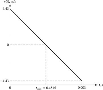
Figure 8.6 The velocity profile of the ball thrown upward.
It should be noted that the derivative of a function is zero both at the points where the value of the function is maximum (maxima) and where the value of the function is minimum (minima). So if the derivative is zero at both maxima and minima, how can one tell whether the value of the function found earlier is a maximum or a minimum? Consider the function shown in Fig. 8.7, which has local maximum and minimum values. As discussed earlier, the derivative of a function at a point is the slope of the tangent line at that point. At its maximum value, the derivative (slope) of the function shown in Fig. 8.7 changes from positive to negative. At its minimum value, the derivative (slope) of the function changes from negative to positive. In other words, the rate of change of the derivative (or the second derivative of the function) is negative at maxima and positive at minima. Therefore, to test for maxima and minima, the following rules apply:
At a Local Maximum:
![]()
At a Local Minimum:
![]()
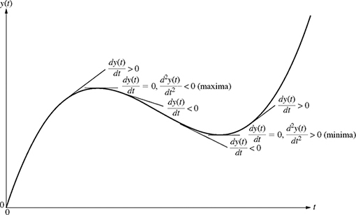
Figure 8.7 Plot of a function with local maximum and minimum values.
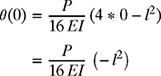
To test whether the point where the slope (first derivative) of the trajectory of the ball thrown upward is zero is a maximum or a minimum, the student obtains the second derivative of the height as
![]()
Therefore, the point where the slope of the trajectory of the ball is zero is a maximum and thus the maximum height is 1.0 m.
In general, the procedure of finding the local maxima and minima of any function f(t) is as follows:
(a) Find the derivative of the function with respect to t; in other words, find ![]()
![]() .
.
(b) Find the solution of the equation f′(t) = 0; in other words, find the values of t where the function has a local maximum or a local minimum.
(c) To find which values of t gives the local maximum and which values of t gives the local minimum, determine the second derivative ![]() of the function.
of the function.
(d) Evaluate the second derivative at the values of t found in step (b). If the second derivative is negative ![]() , the function has a local maximum for those values of t; however, if the second derivative is positive, the function has a local minimum for these values.
, the function has a local maximum for those values of t; however, if the second derivative is positive, the function has a local minimum for these values.
(e) Evaluate the function, f(t), at the values of t found in step (b) to find the maximum and minimum values.
8.3 APPLICATIONS OF DERIVATIVES IN DYNAMICS
This section demonstrates the application of derivatives in determining the velocity and acceleration of an object if the position of the object is given. This section also demonstrates the application of derivatives in sketching plots of position, velocity, and acceleration.
8.3.1 Position, Velocity, and Acceleration
Suppose the position x(t) of an object is defined by a linear function with parabolic blends, as shown in Fig. 8.8. This motion is similar to a vehicle starting from rest and accelerating with a maximum positive acceleration (parabolic position) to reach a constant speed, cruising at that constant speed (linear position), and then coming to stop with maximum braking (maximum negative acceleration, parabolic position).
As discussed previously, velocity v(t) is the instantaneous rate of change of the position (i.e., the derivative of the position) and is given by
![]()
or
![]()
Therefore, the velocity v(t) is the slope of the position x(t) as shown in Fig. 8.9. It can be seen from Fig. 8.9 that the object is starting from rest, moves at a linear velocity with positive slope until it reaches a constant velocity, cruises at that constant velocity, and comes to rest again after moving at a linear velocity with a negative slope.
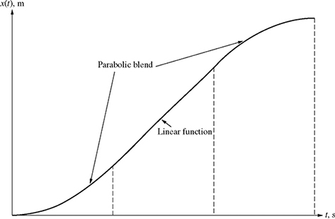
Figure 8.8 Position of an object as a linear function with parabolic blends.
The acceleration a(t) is the instantaneous rate of change of the velocity (i.e., the derivative of the velocity):
![]()

Figure 8.9 Velocity of the object moving as a linear function with parabolic blends.
or
![]()
Therefore, the acceleration a(t) is the slope of the velocity v(t), which is shown in Fig. 8.10. It can be seen from Fig. 8.10 that the object starts with maximum positive acceleration until it reaches a constant velocity, cruises with zero acceleration, and then comes to rest with maximum braking (constant negative acceleration).

Figure 8.10 Acceleration of the object moving as a linear function with parabolic blends.
The following examples will provide some practice in taking basic derivatives using the formulas in Table 8.3.
The motion of the particle shown in Fig. 8.11 is defined by its position x(t). Determine the position, velocity, and acceleration at t = 0.5 seconds if
(a) x(t) = sin (2 πt) m
(b) x(t) = 3 t3 − 4 t2 + 2 t + 6 m
(c) x(t) = 20 cos(3 πt) − 5 t2 m

Solution
(a) The velocity and acceleration of the particle can be obtained by finding the first and second derivatives of x(t), respectively. Since
the velocity is

or
The acceleration of the particle can now be found by differentiating the velocity as

or
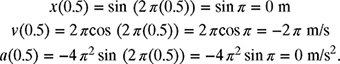
The position, velocity, and acceleration of the particle at t = 0.5 s can now be calculated by substituting t = 0.5 in equations (8.3), (8.4), and (8.5) as
(b) The position of the particle is given by
The velocity of the particle can be calculated by differentiating equation (8.6) as

or
The acceleration of the particle can now be obtained by differentiating equation (8.7) as
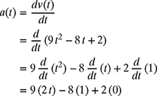
or
The position, velocity, and acceleration of the particle at t = 0.5 s can now be calculated by substituting t = 0.5 in equations (8.6), (8.7), and (8.8) as

(c) The position of the particle is given by
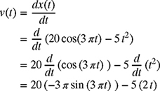
The velocity of the particle can be calculated by differentiating equation (8.9) as
The acceleration of the particle can now be obtained by differentiating equation (8.10) as

or
The position, velocity, and acceleration of the particle at t = 0.5 s can now be calculated by substituting t = 0.5 in equations (8.9), (8.10), and (8.11) as

The following example will illustrate how derivatives can be used to help sketch functions.
The motion of a particle shown in Fig. 8.12 is defined by its position y(t) as
(a) Determine the value of the position and acceleration when the velocity is zero.
(b) Use the results of part (a) to sketch the graph of the position y(t) for 0 ≤ t ≤ 9 s.

Figure 8.12 The position of a particle in the vertical plane.
Solution
(a) The velocity of the particle can be calculated by differentiating equation (8.12) as

or
The time when the velocity is zero can be obtained by setting equation (8.13) equal to zero as
The quadratic equation (8.14) can be solved using one of the methods discussed in Chapter 2. For example, factoring equation (8.14) gives
The two solutions of equation (8.15) are given as:
![]()
Note that quadratic equation (8.14) can also be solved using the quadratic formula, which gives

or
t = 3, 7 s.
Therefore, the velocity is zero at both t = 3 s and t = 7 s. To evaluate the acceleration at these times, an expression for the acceleration is needed. The acceleration of the particle can be obtained by differentiating the velocity of the particle (equation (8.13)) as

or
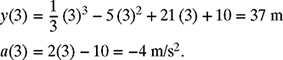
The position and acceleration at time t = 3 s can be found by substituting t = 3 in equations (8.12) and (8.16) as
Similarly, the position and acceleration at t = 7 s can be found by substituting t = 7 in equations (8.12) and (8.16) as

(b) The results of part (a) can be used to sketch the graph of the position y(t). It was shown in part (a) that the velocity of the particle is zero at t = 3 s and t = 7 s. Since the velocity is the derivative of the position, the derivative of the position at t = 3 s and t = 7 s is zero (i.e., the slope is zero). What this means is that the position y(t) has a local minimum or maximum at t = 3 s and t = 7 s. To check whether y(t) has a local minimum or maximum, the second derivative (acceleration) test is applied. Since the acceleration at t = 3 s is negative (a(3) = −4 m/s2), the position y(3) = 37 m is a local maximum. Since the acceleration at t = 7 s is positive (a(7) = 4 m/s2), the position y(7) = 26.3 m is a local minimum. This information, along with the positions of the particle at t = 0 (y(0) = 10 m) and t = 9 (y(9) = 37 m), can be used to sketch the position y(t), as shown in Fig. 8.13.

Figure 8.13 The approximate sketch of the position y(t) of Example 8-2.
Derivatives are frequently used in engineering to help sketch functions for which no equation is given. Such is the case in the following example, which begins with a plot of the acceleration a(t).
The acceleration of a vehicle is measured as shown in Fig. 8.14. Knowing that the particle starts from rest at position x = 0 and travels a total of 16 m, sketch plots of the position x(t) and velocity v(t).
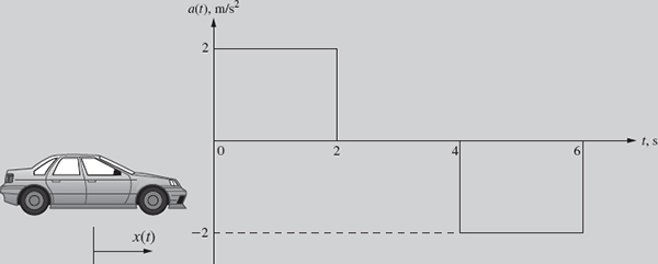
Figure 8.14 Acceleration of a vehicle for Example 8-3.
Solution
(a) Plot of Velocity: The velocity of the vehicle can be obtained from the acceleration profile given in Fig. 8.14. Knowing that v(0) = 0 m/s and ![]() (i.e., a(t) is the slope of v(t)), each interval can be analyzed as follows:
(i.e., a(t) is the slope of v(t)), each interval can be analyzed as follows:

The graph of the velocity profile is shown in Fig. 8.15.
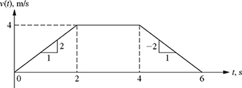
Figure 8.15 The velocity profile for Example 8-3.
(b) Plot of Position: Now, use the velocity, v(t), to construct the position x(t). Knowing that x(0) = 0 m and ![]() (i.e., v(t) is the slope of x(t)), each interval can be analyzed as follows:
(i.e., v(t) is the slope of x(t)), each interval can be analyzed as follows:
(i) 0 ≤ t ≤ 2 s: v(t) is a straight line with a slope of 2 starting from origin (v(0) = 0); therefore, ![]() . From Table 8.3, the position of the vehicle must be a quadratic equation of the form
. From Table 8.3, the position of the vehicle must be a quadratic equation of the form
This can be checked by taking the derivative, for example, ![]()
![]() . Therefore, the equation of position given by (8.17) is correct. The value of C is obtained by evaluating equation (8.17) at t = 0 and substituting the value of x(0) = 0 as
. Therefore, the equation of position given by (8.17) is correct. The value of C is obtained by evaluating equation (8.17) at t = 0 and substituting the value of x(0) = 0 as

Therefore, for 0 ≤ t ≤ 2 s, x(t) = t2 is a quadratic function with a positive slope (concave up) and x(2) = 4 m, as shown in Fig. 8.16.
(ii) 2 < t ≤ 4 s: v(t) has a constant value of 4 m/s, for example, ![]() . Therefore, x(t) is a straight line with a slope of 4 m/s starting with a value of 4 m at t = 2 s as shown in Fig. 8.16. Since the slope is 4 m/s, the position increases by 4 m every second. So during the two seconds between t = 2 and t = 4, its position increases by 8 m. And since the position at time t = 2 s was 4 m, its position at time t = 4 s will be 4 m + 8 m = 12 m. The equation of position for 2 < t ≤ 4 s can be written as
. Therefore, x(t) is a straight line with a slope of 4 m/s starting with a value of 4 m at t = 2 s as shown in Fig. 8.16. Since the slope is 4 m/s, the position increases by 4 m every second. So during the two seconds between t = 2 and t = 4, its position increases by 8 m. And since the position at time t = 2 s was 4 m, its position at time t = 4 s will be 4 m + 8 m = 12 m. The equation of position for 2 < t ≤ 4 s can be written as
x(t) = 4 + 4(t − 2) = 4 t − 4 m.
(iii) 4 < t ≤ 6 s: v(t) is a straight line with a slope of −2 m/s; therefore, x(t) is a quadratic function with decreasing slope (concave down) starting at x(4) = 12 m and ending at x(6) = 16 m with zero slope. The resulting graph of the position is shown in Fig. 8.16.

Figure 8.16 The position of the particle for Example 8-3.
The position of the cart moving on frictionless rollers shown in Fig. 8.17 is given by
x(t) = cos(ωt) m,
where ω = 2 π.
(a) Find the velocity of the cart.
(b) Show that the acceleration of the cart is given by a(t) = −ω2cos(ωt)m/s2, where ω = 2 π.

Solution
(a) The velocity v(t) of the cart is obtained by differentiating the position x(t) as

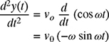
(b) The acceleration a(t) of the cart is obtained by differentiating the position v(t) as

Note that the second derivative of sin(ωt) or cos(ωt) is the same function scaled by −ω2, for example

An object of mass m moving at velocity v0 impacts a cantilever beam (of length l and flexural rigidity EI) as shown in Fig. 8.18. The resulting displacement of the beam is given by
where ![]() is the angular frequency of displacement. Find the following:
is the angular frequency of displacement. Find the following:
(a) The maximum displacement ymax.
(b) The values of the displacement and acceleration when the velocity is zero.

Solution
(a) The maximum displacement can be found by first finding the time tmax when the displacement is maximum. This is done by equating the derivative of the displacement (or the velocity) to zero, (i.e., ![]() ). Since v0 and ω are constants, the derivative is given by
). Since v0 and ω are constants, the derivative is given by

or
Equating equation (8.19) to zero gives
The solutions of equation (8.20) are
![]()
Therefore, the displacement of the beam has local maxima or minima at the values of t given by equation (8.21). To find the time when the displacement is maximum, the second derivative rule is applied. The second derivative of the displacement is obtained by differentiating equation (8.19) as
or
The value of the second derivative of the displacement at ![]() is given by
is given by
![]()
Similarly, the value of the second derivative of the displacement at ![]() is given by
is given by
Therefore, the displacement is maximum at time
![]()
The maximum displacement can be found by substituting ![]() into equation (8.18) as
into equation (8.18) as

or
![]()
Note: The local maxima or minima of trigonometric functions can also be obtained without derivatives. The plot of the beam displacement given by equation (8.18) is shown in Fig. 8.19.

Figure 8.19 Displacement plot to find maximum value.
It can be seen from Fig. 8.19 that the maximum value of the beam displacement is simply the amplitude  and the time where the displacement is maximum is given by
![]()
or
![]()
(b) The position when the velocity is zero is simply the maximum value
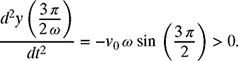
The acceleration found in part (a) is given by a(t) = −v0 ω sin ωt. Therefore, the acceleration when the velocity is zero is given by

Note: ![]() . Therefore, the acceleration is maximum when the displacement y(t) is maximum. Since the second derivative of a sinusoid is also a sinusoid of the same frequency (scaled by −ω2), this is a general result for harmonic motion of any system.
. Therefore, the acceleration is maximum when the displacement y(t) is maximum. Since the second derivative of a sinusoid is also a sinusoid of the same frequency (scaled by −ω2), this is a general result for harmonic motion of any system.
8.4 APPLICATIONS OF DERIVATIVES IN ELECTRIC CIRCUITS
Derivatives play a very important role in electric circuits. For example, the relationship between voltage and current for both the inductor and the capacitor is a derivative relationship. The relationship between power and energy is also a derivative relationship. Before discussing the applications of derivatives in electric circuits, the relationship between different variables in circuit elements is discussed briefly here.
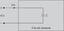
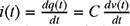
Consider a circuit element as shown in Fig. 8.20, where v(t) is the voltage in volts (V) and i(t) is the current in amperes (A). Note that the current always flows through the circuit element and the voltage is always across the element.

Figure 8.20 Voltage and current in a circuit element.
The voltage v(t) is the rate of change of electric potential energy w(t) (in joules (J)) per unit charge q(t) (in coulomb (C)), that is, the voltage is the derivative of the electric potential energy with respect to charge, written as
![]()
The current i(t) is the rate of change (i.e., derivative) of electric charge per unit time (t in s), written as
![]()
The power p(t) (in watts (W)) is the rate of change (i.e., derivative) of electric energy per unit time, written as
![]()
Note that the power can be written as the product of voltage and current using the chain rule of derivatives:
![]()
The chain rule of derivative is a rule for differentiating composition of functions; for example, if f is a function of g and g is a function of t, then the derivative of composite function f(g(t)) with respect to t can be written as
For example, the function f(t) = sin(2πt) can be written as f(t) = sin(g(t)), where g(t) = 2πt. By the chain rule of equation (8.26),

The chain rule is also useful in differentiating the power of sinusoidal function such as y1(t) = sin2(2πt) or the power of the polynomial function such as y2(t) = (2t + 10)2. The derivatives of these functions are obtained as

and

The following example will illustrate some of the derivative relationships discussed above.
For a particular circuit element, the charge is
and the voltage supplied by the voltage source shown in Fig. 8.21 is

Figure 8.21 Voltage applied to a particular circuit element.
Find the following quantities:
(a) The current, i(t).
(b) The power, p(t).
(c) The maximum power pmax delivered to the circuit element by the voltage source.
Solution
(a) Current: The current i(t) can be determined by differentiating the charge q(t) as

or
(b) Power: The power p(t) can be determined by multiplying the voltage given in equation (8.28) and the current calculated in equation (8.29) as

or
The power p(t) = 250 π sin 500 πt W in equation (8.30) is obtained by using the double-angle trigonometric identity sin(2 θ) = 2sin θ cos θ or ![]() , which gives p(t) = 250 π sin 500 πt.
, which gives p(t) = 250 π sin 500 πt.
(c) Maximum Power Delivered to the Circuit: As discussed in Section 8.3, the maximum value of a trigonometric function such as p(t) = 250 π(sin 500 πt) can be found without differentiating the function and equating the result to zero. Since −1 ≤ sin 500 πt ≤ 1, the power delivered to the circuit element is maximum when sin 500 πt = 1. Therefore,
pmax = 250 πW,
which is simply the amplitude of the power.
8.4.1 Current and Voltage in an Inductor
The current-voltage relationship for an inductor element (Fig. 8.22) is given by
where v(t) is the voltage across the inductor in V, i(t) is the current flowing through the inductor in A, and L is the inductance of the inductor in henry (H). Note that if the inductance is given in mH (1 mH (millihenry) = 10−3 H), it must be converted to H before using it in equation (8.31).

Figure 8.22 Inductor as a circuit element.
For the inductor shown in Fig. 8.22, if L = 100 mH and i(t) = t e−3t A.
(a) Find the voltage ![]() .
.
(b) Find the value of the current when the voltage is zero.
(c) Use the results of (a) and (b) to sketch the current i(t).
(a) The voltage v(t) is determined as

or
![]()
where ![]() . To differentiate the product of two functions (t and e−3t), the product rule of differentiation (Table 8.3) is used:
. To differentiate the product of two functions (t and e−3t), the product rule of differentiation (Table 8.3) is used:
Substituting f(t) = t and g(t) = e−3t in equation (8.32) gives
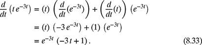
Therefore,
(b) To find the current when the voltage is zero, first find the time t when the voltage is zero and then substitute this time in the expression for current. Setting equation (8.34) equal to zero gives
0.1 e−3t (−3 t + 1) = 0.
Since e−3t is never zero, it follows that (−3 t + 1) = 0, which gives t = 1/3 sec. Therefore, the value of the current when the voltage is zero is determined by substituting t = 1/3 into the current i(t) = t e−3t, which gives

or
i = 0.123 A.
(c) Since the voltage is proportional to the derivative of the current, the slope of the current is zero when the voltage is zero. Therefore, the current i(t) is maximum (imax = 0.123 A) at t = 1/3 s. Also, at t = 0, i(0) = 0 A. Using these values along with the values of the current at t = 1 s (i(1s) = 0.0498 A) and at t = 2 s (i(2s) = 0.00496 A), the approximate sketch of the current can be drawn as shown in Fig. 8.23. Note that i = 0.123 A must be a maximum (as opposed to a minimum) value, since it is the only location of zero slope and is greater than the values of i(t) at either t = 0 or t = 2 s. Hence, no second derivative test is required!

Figure 8.23 Approximate sketch of the current waveform for Example 8-7.
As seen in dynamics, derivatives are frequently used in circuits to sketch functions for which no equations are given, as illustrated in the following example:
For the given input voltage (square wave) shown in Fig. 8.24, plot the current i(t) and the power p(t) if L = 500 mH. Assume i(0) = 0 A and p(0) = 0W.

Solution
For an inductor, the current-voltage relationship is given by ![]() . Since the voltage is known, the rate of change of the current is given by
. Since the voltage is known, the rate of change of the current is given by
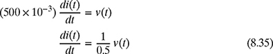
or
![]()
Therefore, the slope of the current is twice the applied voltage. Since v(t) = ± 9 V (constant in each interval), the current waveform has a constant slope of ± 18 A/s, in other words, the current waveform is a straight line with a constant slope of ± 18 A/s. In the interval 0 ≤ t ≤ 2, the current waveform is a straight line with a slope of 18 A/s that starts at 0 A (i(0) = 0 A). Therefore, the value of the current at t = 2 s is 36 A. In the interval, 2 < t ≤ 4, the current waveform is a straight line starting at 36 A (at t = 2 s) with a slope of −18 A/s. Therefore, the value of the current at t = 4 s is 0 A. This completes one cycle of the current waveform. Since the value of the current at t = 4 s is 0 (the same as at t = 0 s) and the applied voltage between interval 4 < t ≤ 8 is the same as the applied voltage between 0 ≤ t ≤ 4, the waveform for the current from 4 ≤ t ≤ 8 is the same as the waveform of the current from 0 ≤ t ≤ 4. The resulting plot of i(t) is shown in Fig. 8.25. Hence, when a square wave voltage is applied to an inductor, the resulting current is a

Figure 8.25 Sketch of the current waveform for Example 8-8.
triangular wave. Since p(t) = v(t) i(t) and the voltage is ± 9 V, the power is given by p(t) = (± 9) i(t) W. In the interval 0 ≤ t ≤ 2, v(t) = 9 V, therefore, p(t) = 9 i(t) W. The waveform of the power is a straight line starting at 0 W with a slope of (9 × 18) = 162 W/s. Therefore, the power delivered to the inductor just before t = 2 sec is 324 W. Just after t = 2 sec, the voltage is −9 V and the current is 36 A. Thus, the power jumps down to (−9) (36) = −324 W. In the interval 2 < t ≤ 4, v(t) = −9 V, and the current has a negative slope of −18 A/s. Therefore, the waveform for the power is a straight line starting at −324 W with a slope of 162 W/s. Thus, p(4) = −324 + 2(162) = 0 W. This completes one cycle of the power. Since the value of the power at t = 4 s is 0 (the same as at t = 0 s) and the applied voltage and current in the interval 4 ≤ t ≤ 8 are the same as the voltage and current in the 0 ≤ t ≤ 4, the waveform for the power from 4 ≤ t ≤ 8 is the same as the waveform of the power from 0 ≤ t ≤ 4. The resulting plot of p(t) is shown in Fig. 8.26, and is typically referred to as a sawtooth curve.

Figure 8.26 Sketch of the power for Example 8-8.
8.4.2 Current and Voltage in a Capacitor
The current-voltage relationship for a capacitive element (Fig. 8.27) is given by
where v(t) is the voltage across the capacitor in V, i(t) is the current flowing through the capacitor in A, and C is the capacitance of the capacitor in farad (F). Note that if the capacitance is given in μF (10−6 F), it must be converted to F before using it in equation (8.36).
Example 8-9
Consider the capacitive element shown in Fig. 8.27 with C = 25 μF and v(t) = 20 e−500t sin 5000 πt V. Find the current i(t).
Solution The current i(t) can be found by using equation (8.36) as
![]()
Substituting the value of C gives
![]()
where ![]() . To differentiate the product of the two functions e−500 t and sin 5000 πt, the product rule of differentiation is required. Letting f(t) = e−500 t and g(t) = sin 5000 πt,
. To differentiate the product of the two functions e−500 t and sin 5000 πt, the product rule of differentiation is required. Letting f(t) = e−500 t and g(t) = sin 5000 πt,
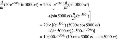
Therefore,
i(t) = 25 × 10−6 (10,000 e−500t (10 πcos 5000 πt − sin 5000 πt))
or
i(t) = 0.25 e−500 t (10 πcos 5000 πt − sin 5000 πt) A
Using the results of Chapter 6, this can also be written as i(t) = 2.5 πe−500 t sin(5000 πt + 92°) A.
The current shown in Fig. 8.28 is used to charge a capacitor with C = 20 μF. Knowing that ![]() , plot the charge q(t) stored in the capacitor and the corresponding voltage v(t). Assume q(0) = v(0) = 0.
, plot the charge q(t) stored in the capacitor and the corresponding voltage v(t). Assume q(0) = v(0) = 0.

(a) Charge: Since ![]() , the slope of the charge q(t) is given by each constant value of current in each interval, for example
, the slope of the charge q(t) is given by each constant value of current in each interval, for example
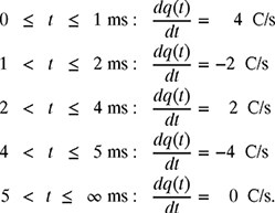
Therefore, the plot of the charge q(t) stored in the capacitor can be drawn as shown in Fig. 8.29. Note that since time t is in ms, the charge q(t) is in mC.

Figure 8.29 Charge on the capacitor in Example 8-10.
(b) Voltage: To find the voltage across the capacitor, the relationship between the charge and the voltage is first derived as:
![]()
Therefore, the derivative (slope) of the voltage v(t) is equal to the derivative (slope) of the charge q(t) multiplied by the reciprocal of the capacitance. Substituting the value of C gives
![]()
or
![]()
The plot of the voltage is thus the same as the plot of the charge with the ordinate scaled by 50 × 103, as shown in Fig. 8.30.
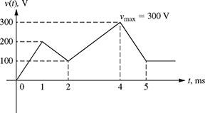
Figure 8.30 Voltage across the capacitor.
Note that while the time is still measured in ms, the voltage is measured in volts.
8.5 APPLICATIONS OF DERIVATIVES IN STRENGTH OF MATERIALS
In this section, the derivative relationship for beams under transverse loading conditions will be discussed. The locations and values of maximum deflections are obtained using derivatives, and results are used to sketch the deflection. This section also considers the application of derivatives to maximum stress under axial loading and torsion.
Consider a beam with elastic modulus E (lb/in.2 or N/m2) and second moment of area I (in.4 or m4) as shown in Fig. 8.31. The product EI is called the flexural rigidity and is a measure of how stiff the beam is. If the beam is loaded with a distributed transverse load q(x) (lb/in. or N/m), the beam deflects in the y-direction with a deflection of y(x) (in. or m) and a slope of ![]() in radians.
in radians.

Figure 8.31 A beam loaded in the y-direction.
The internal moments and forces in the beam shown in Fig. 8.32 are given by the expressions

Figure 8.32 The internal forces in a beam loaded by a distributed load.
More detailed background on the above relations can be found in any book on strength of materials.
Example 8-11
Consider a cantilever beam of length l loaded by a force P at the free end, as shown in Fig. 8.33. If the deflection is given by
find the deflection and slope at the free end x = l.

Solution
Deflection: The deflection of the beam at the free end can be determined by substituting x = l in equation (8.40), which gives

or
![]()
This classic result is used in a range of mechanical and civil engineering courses.
Slope: The slope of the deflection θ(x) can be found by differentiating the deflection y(x) as

or
Note that the parameters P, l, E, and I are all treated as constants.
The slope θ(x) at the free end can now be determined by substituting x = l in. equation (8.41) as

or
![]()
Note: It can be seen by inspection that both the deflection and the slope of deflection are maximum at the free end, for example:

It can be seen that doubling the load P would increase the maximum deflection and slope by a factor of 2. However, doubling the length l would increase the maximum deflection by a factor of 8, and the maximum slope by a factor of 4!
Example 8-12
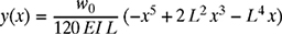
Consider a simply supported beam of length l subjected to a central load P, as shown in Fig. 8.34. For 0 ≤ x ≤ 1/2, the deflection is given by
Determine the maximum defection ymax, as well as the slope at the end x = 0.

Solution
The deflection is maximum when ![]() . The slope of the deflection can be found as
. The slope of the deflection can be found as

or
To find the location of the maximum deflection, θ(x) is set to zero and the resulting equation is solved for the values of x as
![]()
Since the deflection is given for 0 ≤ x ≤ l/2, the deflection is maximum at x = l/2. The value of the maximum deflection can now be found by substituting x = l/2 in equation (8.42) as

or
![]()
Likewise, the slope θ(x) at x = 0 can be determined by substituting x = 0 in equation (8.43) as
or
![]()
Example 8-13
A simply supported beam of length l is subjected to a distributed load ![]() as shown in Fig. 8.35. If the deflection is given by
as shown in Fig. 8.35. If the deflection is given by
find the slope θ(x), the moment M(x) and the shear force V(x).

Slope: The slope of the deflection θ(x) is given by

or
Moment: By definition, the moment M(x) is obtained by multiplying the derivative of the slope θ(x) by EI, or
![]()
Substituting equation (8.45) for θ(x) gives

or
Shear Force: By definition, the shear force V(x) is the derivative of the moment M(x), or
![]()
Substituting equation (8.46) for M(x) gives

The above answer can be checked by showing that ![]() as
as

or
which matches the applied load in Fig. 8.35.
8.5.1 Maximum Stress under Axial Loading
In this section, the application of derivatives in finding maximum stress under axial loading is discussed. A normal stress σ results when a bar is subjected to an axial load P (through the centroid of the cross section), as shown in Fig. 8.36. The normal stress is given by
where A is the cross-sectional area of the section perpendicular to longitudinal axis of the bar. Therefore, the normal stress σ acts perpendicular to the cross section and has units of force per unit area (psi or N/m2).

Figure 8.36 A rectangular bar under axial loading.
To find the stress on an oblique plane, consider an inclined section of the bar as shown in Fig. 8.37.

Figure 8.37 Inclined section of the rectangular bar.
The relationship between the cross-sectional area perpendicular to the longitudinal axis and the area of the inclined plane is given by
The force P can be resolved into components perpendicular to the inclined plane F and parallel to the inclined plane V. The free-body diagram of the forces acting on the oblique plane is shown in Fig. 8.38. Note that the resultant force in the axial direction must be equal to P to satisfy equilibrium.

Figure 8.38 Free-body diagram.
The relationship among P, F, and V can be found by using the right triangle shown in Fig. 8.39 as
![]()

Figure 8.39 Triangle showing force P, F, and V.
The force perpendicular to the inclined cross section F produces a normal stress σθ (shown in Fig. 8.40) given by


Figure 8.40 Normal and shear stresses acting on the inclined cross section.
The tangential force V produces a shear stress τθ given as

Substituting ![]() from (8.49) into equations (8.50) and (8.51), the normal and shear stresses on the inclined cross section are given by
from (8.49) into equations (8.50) and (8.51), the normal and shear stresses on the inclined cross section are given by
In general, brittle materials like glass, concrete, and cast iron fail due to maximum values of σθ (normal stress). However, ductile materials like steel, aluminum, and brass fail due to maximum values of τθ (shear stress).
Example 8-14
Use derivatives to find the values of θ where σθ and τθ are maximum, and find their maximum values.
Solution
(a) First, find the derivative of σθ with respect to θ: The derivative of σθ given by equation (8.52) is

(b) Next, equate the derivative in equation (8.54) to zero and solve the resulting equation for the value of θ between 0 and 90° where σθ is maximum. Therefore, −2 cos θ sin θ = 0, which gives
cos θ = 0 ⇒ θ = 90°
or
sin θ = 0 ⇒ θ = 0°.
Therefore, θ = 0° and 90° are the critical points; in other words, at θ = 0° and 90°, σθ has a local maximum or minimum. To find the value of θ where σθ has a maximum, the second derivative test is performed. The second derivative of σθ is given by

or
![]()
where cos 2 θ = cos2 θ − sin2 θ. For θ = 0°, ![]() . So σθ has a maximum value at θ = 0°.
. So σθ has a maximum value at θ = 0°.
For θ = 90°, ![]() ; therefore, σθ has a minimum value at θ = 90°.
; therefore, σθ has a minimum value at θ = 90°.
Maximum Value of σθ: Substituting θ = 0° in equation (8.52) gives
σmax = σ cos2 (0°) = σ.
This means that the largest normal stress during axial loading is simply the applied stress σ!
Value of θ where τθ is maximum:
(a) First, find the derivative of τθ with respect to θ: The derivative of τθ given by equation (8.53) is given by

or
(b) Next, equate the derivative in equation (8.55) to zero and solve the resulting equation σ cos 2 θ = 0 for the value of θ (between 0 and 90°) where τθ is maximum:
cos 2 θ = 0 ⇒ 2 θ = 90° ⇒ θ = 45°.
Therefore, τθ has a local maximum or minimum at θ = 45°. To find whether τθ has a maximum or minimum at θ = 45°, the second derivative test is performed. The second derivative of τθ is given by

For 0 ≤ θ ≤ 90° ⇒ 0 ≤ 2 θ ≤ 180° ⇒ sin 2 θ > 0, therefore, ![]() . Since the second derivative is negative, τθ has a maximum value at θ = 45°.
. Since the second derivative is negative, τθ has a maximum value at θ = 45°.
Maximum Value of τθ: Substituting θ = 45° in equation (8.53) gives

or
![]()
Thus, the maximum shear stress during axial loading is equal to half the applied normal stress, but at an angle of 45°. This is why a tensile test of a steel specimen results in failure at a 45° angle.
8.6 FURTHER EXAMPLES OF DERIVATIVES IN ENGINEERING
Example 8-15
The velocity of a skydiver jumping from a height of 12,042 ft is shown in Fig. 8.41.
(a) Find the equation of the velocity v(t) for the five time intervals shown in Fig. 8.41.
(b) Knowing that ![]() , find the acceleration a(t) of the skydiver for 0 ≤ t ≤ 301 s.
, find the acceleration a(t) of the skydiver for 0 ≤ t ≤ 301 s.
(c) Use the results of part (b) to sketch the acceleration a(t) for 0 ≤ t ≤ 301 s.

Figure 8.41 Velocity profile of the skydiver jumping from a height of 12,042 ft.
Solution
(a)
(i) 0 ≤ t ≤ 5 s: v(t) is linear with slope

Therefore, v(t) = −32.2 t ft/s.
(ii) 5 < t ≤ 28 s: v(t) is constant at
v(t) = −161 ft/s.
(iii) 28 < t ≤ 31 s: v(t) is linear with slope

Therefore, v(t) = 43.67 t + b ft/s. The value of b (y-intercept) can be found by substituting the data point (t, v(t)) = (31, −30), which gives
−30 = 43.67(31) + b ⇒ b = −1383.67
Therefore, v(t) = 43.67 t − 1383.67 ft/s.
(iv) 31 < t ≤ 271 s: v(t) is constant at
v(t) = −30 ft/s.
(v) 271 < t ≤ 301 s: v(t) is linear with slope

Therefore, v(t) = t + b ft/s. The value of b (y-intercept) can be found by substituting the data point (t, v(t)) = (301, 0), which gives
0 = 1(301) + b ⇒ b = −301
Therefore, v(t) = t − 301 ft/s.
(b)
(i) 0 ≤ t ≤ 5 s:

(ii) 5 < t ≤ 28 s:

(iii) 28 < t ≤ 3 s:


(v) 271 < t ≤ 301 s:

(c) The acceleration of the skydiver found in part (b) can be drawn as shown in Fig. 8.42.

Figure 8.42 The acceleration of the skydiver.
Example 8-16
A proposed highway traverses a hilltop bounded by uphill and downhill grades of 10% and −8%, respectively. These grades pass through benchmarks A and B located as shown in Fig. 8.43. With the origin of the coordinate axes (x, y) set at benchmark A, the engineer has defined the hilltop segment of the highway by a parabolic arc:
which is tangent to the uphill grade at the origin.
(a) Find the slope of the line for the uphill grade and the value of b for the parabolic arc.
(b) Find the equation of the line
for the downhill grade.
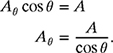
(c) Given that at the downhill point of tangency (![]() ), both the elevation and the slope of the parabolic arc are equal to their respective values of the downhill line:
), both the elevation and the slope of the parabolic arc are equal to their respective values of the downhill line:
Determine the point of tangency ![]() of the parabolic arc with the downhill grade. Also, compute its elevation.
of the parabolic arc with the downhill grade. Also, compute its elevation.
(d) Find the equation of the parabolic arc.

Solution
(a) The initial slope of the parabolic arc is equal to the uphill grade, which is expressed as a decimal fraction of 0.1. Since the arc is tangent to the uphill grade at the origin, the initial slope is equal to the derivative of equation (8.56) evaluated at x = 0. The derivative of the parabolic arc is given by

Therefore, the slope of the line for the uphill grade can be found by setting x = 0 in equation (8.60) as
Hence, the initial slope of the arc is given by the coefficient b of the equation (8.56) and has the value b = 0.1.
(b) The slope of the line (equation (8.57)) for the downhill grade is given by c = −0.08. Therefore, the equation of the line can be written as
Since this line passes through benchmark B, the value of the y-intercept d can be found by substituting the data point (200, −6) into equation (8.62) as

Therefore, the equation of the line for the downhill slope is given by
(c) Substituting ![]() in equation (8.60) gives
in equation (8.60) gives
Evaluating the derivative of equation (8.63) at ![]() gives
gives
Substituting equations (8.64) and (8.65) into equation (8.59) gives
Evaluating equations (8.56) and (8.62) at ![]() and substituting the results in equation (8.58) gives
and substituting the results in equation (8.58) gives
Now, substituting the value of ![]() from equation (8.66) into equation (8.67), the value of
from equation (8.66) into equation (8.67), the value of ![]() can be found as
can be found as

Thus, the point of tangency lies a horizontal distance of 111.1 m from benchmark A. Its elevation ![]() is obtained by substituting this value of
is obtained by substituting this value of ![]() into equation (8.63) as
into equation (8.63) as

Therefore, the downhill point of tangency is given by (111.1, 1.11) m.
(d) With the value of ![]() known, the coefficient a for the parabolic arc can be obtained from equation (8.66) as
known, the coefficient a for the parabolic arc can be obtained from equation (8.66) as

The equation for the parabolic arc may now be written by substituting the values of a and b from equations (8.70) and (8.61) into equation (8.56) as
y = −0.00081 x2 + 0.1 x.
-
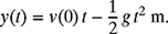
8-1. A model rocket is fired from the roof of a 50 ft tall building as shown in Fig. P8.1. The height of the rocket is given by

where y(t) is the height of the rocket at time t, y(0) = H = 50 ft is the initial height of the rocket, v(0) = 150 ft/s is the initial velocity of the rocket, and g = 32.2 ft/s2 is the acceleration due to gravity. Find the following:
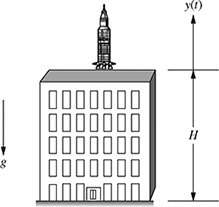
Figure P8.1 A rocket fired from top of a building in problem P8-1.
(a) Write the quadratic equation for the height y(t) of the rocket.
(b) The velocity
 .
.(c) The acceleration

 .
.(d) The time required to reach the maximum height as well as the corresponding height ymax. Use your results to sketch y(t).
-
8-2. Repeat problem P8-1 if H = 15m, v(0) = 49 m/s and g = 9.8 m/2.
-
8-3. The height in the vertical plane of a ball thrown from the ground with an initial velocity of v(0) = 250 m/s satisfies the relationship
where g = 9.8 m/s2 is the acceleration due to gravity.

Figure P8.3 A projectile in the vertical plane.
Find the following:
(a) Write the quadratic equation for the height y(t) of the ball.
(b) The velocity
 .
.(c) The acceleration

 .
.(d) The time required to reach the maximum height, as well as the corresponding height ymax. Use your results to sketch y(t).
-
8-4. Repeat problem P8-3 if v(0) = 161 ft/s and g= 32.2 ft/s2.
-
8-5. The motion of a particle moving in the horizontal direction as shown in Fig. P8.5 is described by its position x(t). Determine the position, velocity, and acceleration at t = 3.0 s if

Figure P8.5 A particle moving in the horizontal direction.
(a)
 .
.(b)
 .
.(c) x(t) = 2 e4 t + 3 e−5 t + 2 (et − 1) m.
-
8-6. The motion of a particle moving in the horizontal direction is described by its position x(t). Determine the position, velocity, and acceleration at t = 1.5 s if
(a) x(t) = 4 cos(5 πt) m.
(b) x(t) = 4 t3 − 6 t2 + 7 t + 2 m.
(c) x(t) = 10 sin(10 πt) + 5 e3 t m.
-
8-7. The motion of a particle in the vertical plane is shown in Fig. P8.7. The height of the particle is given by
y(t) = t3 − 12 t2 + 36 t + 20 m.
(a) Find the values of position and acceleration when the velocity is zero.
(b) Use your results in part (a) to sketch y(t) for 0 ≤ t ≤ 9 s.

-
8-8. The motion of a particle in the vertical plane is shown in Fig. P8.8. The height of the particle is given by
y(t) = 2 t3 − 15 t2 + 24 t + 8 m
(a) Find the values of the position and acceleration when the velocity is zero.
(b) Use your results in part (a) to sketch y(t) for 0 ≤ t ≤ 4 s.
-
8-9. The voltage across an inductor is given by
 . If i(t) = t3 e−2 t A and L = 0.125 H,
(a) Find the voltage, v(t).
(b) Find the value of the current when the voltage is zero.
(c) Use the above information to sketch i(t).

-
8-10. Repeat problem P8-9 if L = 0.25 H and i(t) = t2 e−t A.
-
8-11. The voltage across the inductor of Fig. P8.9 is given by
 . Determine the voltage v(t), the power p(t) = v(t) i(t), and the maximum power transfered if the inductance is L = 2 mH and the current i(t) is given by
(a) i(t) = 13 e−200 t A.
(b) i(t) = 20 cos(2 π60t) A.
-
8-12. The current flowing through a capacitor shown in Fig. P8.12 is given by
 . If C = 500 μF and v(t) = 250 sin(200 πt) V,
(a) Find the current i(t).
(b) Find the power p(t) = v(t) i(t) and its maximum value pmax.

-
8-13. Repeat problem P8-12 if C = 40 μF and v(t) = 500 cos(200 πt) V.
-
8-14. The current flowing through the capacitor shown in Fig. P8.12 is given by
 . If C = 2 μF and v(t) = t2 e−10 t V,
(a) Find the current i(t).
(b) Find the value of the voltage when the current is zero.
(c) Use the given information to sketch v(t).
-
8-15. A vehicle starts from rest at position x = 0. The velocity of the vehicle for the next 8 seconds is shown in Fig. P8.15.
(a) Knowing that
 , sketch the acceleration a(t).
(b) Knowing that
 , sketch the position x(t) if the minimum position is x = −16 m and the final position is x = 0.
 -
8-16. At time t = 0, a vehicle located at position x = 0 is moving at a velocity of 10 m/s. The velocity of the vehicle for the next 8 seconds is shown in Fig. P8.16.
(a) Knowing that
 , sketch the acceleration a(t).
(b) Knowing that
 , sketch the position x(t) if the maximum position is x = 30 m and the final position is x = 10 m.
Figure P8.15 Velocity of a vehicle for problem P8-15.

-
8-17. At time t = 0, a moving vehicle is located at position x = 0 and subjected to the acceleration a(t) shown in Fig. P8.17.

Figure P8.17 Acceleration of a vehicle for problem P8-17.
(a) Knowing that
 , sketch the velocity v(t) if the initial velocity is 12 m/s.
(b) Knowing that
 , sketch the position x(t) if the final position is x = 48 m.
 -
8-18. A vehicle starting from rest at position x = 0 is subjected to the acceleration a(t) shown in Fig. P8.18.
(a) Knowing that
 , sketch the velocity v(t).
(b) Knowing that
 , sketch the position x(t) if the final position is x = 60 m. Clearly indicate both its maximum and final values.
 -
8-19. A vehicle starting from rest at position x = 0 is subjected to the following acceleration a(t):
Figure P8.18 Acceleration of a vehicle for problem P8-18.

Figure P8.19 Acceleration of a vehicle for problem P8-19.
(a) Knowing that
 , sketch the velocity v(t).
(b) Knowing that
 , sketch the position x(t) if the final position is x = 15 m. Clearly indicate both its maximum and final values.
 -
8-20. A vehicle starting from rest at position x = 0 is subjected to the following acceleration a(t):

Figure P8.20 Acceleration of a vehicle for problem P8-20.
(a) Knowing that
, sketch the velocity v(t).(b) Knowing that
, sketch the position x(t) if the final position is x = 260 m. Clearly indicate both its maximum and final values. -
8-21. The voltage across an inductor is given in Fig. P8.21. Knowing that
 and p(t) = v(t) i(t), sketch the graphs of i(t) and p(t). Assume L = 2 H, i(0) = 0A, and p(0) = 0W.
 -
8-22. The voltage across an inductor is given in Fig. P8.22. Knowing that
 and p(t) = v(t) i(t), sketch the graphs of i(t) and p(t). Assume L = 0.25 H, i(0) = 0 A, and p(0) = 0 W.
-
8-23. The voltage across an inductor is given in Fig. P8.23. Knowing that
 and p(t) = v(t) i(t), sketch the graphs of i(t) and p(t). Assume L = 2 mH, i(0) = 0A, and p(0) = 0W.
-
8-24. The current applied to a capacitor is given in Fig. P8.24. Knowing that
 , sketch the graphs of the stored charge q(t) and the voltage v(t). Assume C = 250 μF, q(0) = 0 C, and v(0) = 0 V.
Figure P8.24 Current flowing through a capacitor for problem P8-24.
-
8-25. The current flowing through a capacitor is given in Fig. P8.25. Knowing that
 , sketch the graphs of the stored charge q(t) and the voltage v(t). Assume C = 250 μF, q(0) = 0C, and v(0) = 0 V.
Figure P8.25 Current flowing through a capacitor for problem P8-25.
-
8-26. The current flowing through a 500 μF capacitor is given in Fig. P8.26. Knowing that
 , plot v(t) for 0 ≤ t ≤ 4 sec if v(0) = −4 V, v(2) = 2 V, v(4) = 2 V, and the maximum voltage is 4 V.
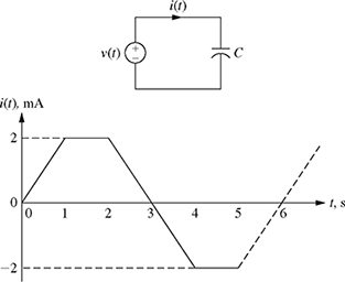
Figure P8.26 Current flowing through a capacitor for problem P8-26.
-
8-27. A simply supported beam is subjected to a load P as shown in Fig. P8.27. The deflection of the beam is given by
 ,
, 
where EI is the flexural rigidity of the beam. Find the following:
(a) The location and the value of maximum deflection ymax.
(b) The value of the slope
 at the end x = 0.
-
8-28. A simply supported beam is subjected to a load P at
 as shown in Fig. P8.28. The deflection of the beam is given by
 ,
, 
where EI is the flexural rigidity of the beam. Find the following:
(a) The equation of the slope
.(b) The location and magnitude of maximum deflection ymax.
(c) Evaluate both the deflection and slope at x = 0 and
 .
.(d) Use the results of parts (b) and (c) to sketch the deflection y(x) for
 .
. -
8-29. A simply supported beam is subjected to an applied moment Mo at its center
 as shown in Fig. P8.29. The deflection of the beam is given by
 ,
, 
where EI is the flexural rigidity of the beam. Find the following:
(a) The equation for the slope
 .
.(b) The location and the value of maximum deflection ymax.
(c) Evaluate both the deflection and slope at the points A and B (x = 0 and
 ).
).(d) Use the results of parts (a)–(c) to sketch the deflection y(x) from x = 0 to
.
-
8-30. A simply supported beam is subjected to a sinusoidal distributed load, as shown in the Fig. P8.30. The deflection y(x) of the beam is given by

where EI is the flexural rigidity of the beam. Find the following:

Figure P8.30 A simply supported beam for problem P8-30.
(a) The equation for the slope
 .
.(b) The value of the slope where the deflection is zero.
(c) The value of the deflection at the location where the slope is zero.
(d) Use the results of parts (b) and (c) to sketch the deflection y(x).
-
8-31. Consider a beam under a linear distributed load and supported as shown in Fig. P8.31. The deflection of the beam is given by
where L is the length and EI is the flexural rigidity of the beam. Find the following:
(a) The location and value of the maximum deflection ymax.
(b) The value of the slope
 at the ends x = 0 and x = L.
(c) Use your results in (a) and (b) to sketch the deflection y(x).
Figure P8.31 A beam under linear distributed load for problem P8-31.
-
8-32. A fixed-fixed beam is subjected to a sinusoidal distributed load, as shown in Fig. P8.32.

Figure P8.32 A fixed-fixed beam subjected to a sinusoidal distributed load.
The deflection y(x) is given by
 .
.(a) Determine the equation for the slope
.(b) Evaluate both the deflection and the slope at the points x = 0 and x = L.
(c) Determine both the location and value of the maximum deflection.
(d) Use your results of parts (b) and (c) to sketch the deflection y(x), and clearly indicate both the location and value of the maximum deflection.
-
8-33. Consider the buckling of a pinned-pinned column under a compressive axial load P as shown in Fig. P8.33.

Figure P8.33 A pinned-pinned column under a compressive axial load.
The deflection y(x) of the second buckling mode is given by
 , where A is an undetermined constant.
(a) Determine the equation for the slope
.(b) Determine the value of the slope at the locations where the deflection is zero.
(c) Determine the value of the deflection at the locations where the slope is zero.
(d) Use your results of parts (b) and (c) to sketch the buckled deflection y(x).
-
8-34. Consider the buckling of a pinned-fixed column under a compressive load P as shown in Fig. P8.34.
The deflection y(x) of the buckled configuration is given by

where A is an undetermined constant.
(a) Determine the equation for the slope
 .
.Figure P8.34 A pinned-fixed column under a compressive load.
(b) Evaluate both the deflection and the slope at the points x = 0 and x = L.
(c) Determine the location and magnitude of the maximum deflection.
(d) Use your results of parts (b) and (c) to sketch the buckled deflection y(x).
-
8-35. Consider a beam under a uniform distributed load and supported as shown in Fig. P8.35. The deflection of the beam is given by

where L is the length and EI is the flexural rigidity of the beam. Find the following:

Figure P8.35 A beam under uniform distributed load for problem P8-35.
(a) The location and value of the maximum deflection ymax.
(b) The value of the slope
 at the ends x = 0 and x = L.
(c) Use your results in (a) and (b) to sketch the deflection y(x).
-
8-36. A cantilever beam is pinned at the end x = L, and subjected to an applied moment Mo as shown in Fig. P8.36. The deflection y(x) of the beam is given by

where L is the length and EI is the flexural rigidity of the beam. Find the following:
(a) The equation of the slope
.(b) The location and magnitude of the maximum deflection ymax.
(c) Evaluate both the deflection and slope at the points A and B (x = 0 and x = L).
(d) Use the results in parts (b) and (c) to sketch the deflection y(x) and clearly indicate the location of the maximum deflection on the sketch.

-
8-37. Consider a shaft subjected to an applied torque T, as shown in Fig. P8.37. The internal normal and shear stresses at the surface vary with the angle relative to the axis and are given by equations (8.71) and (8.72), respectively.
Find
(a) the angle θ where σθ is maximum
(b) the angle θ where τθ is maximum

-
8-38. The velocity of a skydiver jumping from a height of 13,000 ft is shown in Fig. P8.38.
(a) Find the equation of the velocity v(t) for the five time intervals shown in Fig. P8.38.
(b) Knowing that
 , sketch the acceleration a(t) of the skydiver for 0 ≤ t ≤ 180 s.
(c) Use the results of part (b) to sketch the height y(t) for 0 ≤ t ≤ 180 s.
-
8-39. A proposed highway traverses a hilltop bounded by uphill and downhill grades of 15% and −10%, respectively. These grades pass through benchmarks A and B located as shown in Fig. P8.39. With the origin of the coordinate axes (x, y) set at benchmark A, the engineer has defined the hilltop segment of the highway by a parabolic arc
y(x) = ax2 + bx,
which is tangent to the uphill grade at the origin.
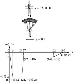
Figure P8.38 Velocity of a skydiver jumping from a height of 13,000 ft.
(a) Find the slope of the line for the uphill grade and the value of b for the parabolic arc.
(b) Find the equation of the line

for the downhill grade.
(c) Given that at the downhill point of tangency
 , both the elevation and the slope of the parabolic arc are equal to their respective values of the downhill line, for example,
Figure P8.39 Parabolic arc traversing highway hilltop.
determine the point of tangency
 of the parabolic arc with the downhill grade. Also, compute its elevation.
(d) Find the equation of the parabolic arc.


