Straight Lines in Engineering |
CHAPTER 1 |
In this chapter, the applications of straight lines in engineering are introduced. It is assumed that the students are already familiar with this topic from their high school algebra course. This chapter will show, with examples, why this topic is so important for engineers. For example, the velocity of a vehicle while braking, the voltage-current relationship in a resistive circuit, and the relationship between force and displacement in a preloaded spring can all be represented by straight lines. In this chapter, the equations of these lines will be obtained using both the slope-intercept and the point-slope forms.
1.1 VEHICLE DURING BRAKING
The velocity of a vehicle during braking is measured at two distinct points in time, as indicated in Fig. 1.1.
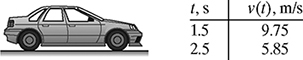
Figure 1.1 A vehicle while braking.
The velocity satisfies the equation
where vo is the initial velocity in m/s and a is the acceleration in m/s2.
(a) Find the equation of the line v(t) and determine both the initial velocity vo and the acceleration a.
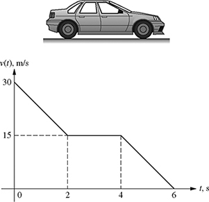
(b) Sketch the graph of the line v(t) and clearly label the initial velocity, the acceleration, and the total stopping time on the graph.
The equation of the velocity given by equation (1.1) is in the slope-intercept form y = mx + b, where y = v(t), m = a, x = t, and b = vo. The slope m is given by
![]()
Therefore, the slope m = a can be calculated using the data in Fig. 1.1 as
![]()
The velocity of the vehicle can now be written in the slope-intercept form as
v(t) = −3.9 t + vo.
The y-intercept b = vo can be determined using either one of the data points. Using the data point (t, v) = (1.5, 9.75) gives
9.75 = −3.9 (1.5) + vo.
Solving for vo gives
vo = 15.6 m/s.
The y-intercept b = vo can also be determined using the other data point (t, v) = (2.5, 5.85), yielding
5.85 = −3.9 (2.5) + vo.
Solving for vo gives
vo = 15.6 m/s.
The velocity of the vehicle can now be written as
v(t) = −3.9 t + 15.6 m/s.
The total stopping time (time required to reach v(t) = 0) can be found by equating v(t) = 0, which gives
0 = −3.9 t + 15.6.
Solving for t, the stopping time is found to be t = 4.0 s. Figure 1.2 shows the velocity of the vehicle after braking. Note that the stopping time t = 4.0 s and the initial velocity vo = 15.6 m/s are the x- and y-intercepts of the line, respectively. Also, note that the slope of the line m = −3.90 m/s2 is the acceleration of the vehicle during braking.

Figure 1.2 Velocity of the vehicle after braking.
1.2 VOLTAGE-CURRENT RELATIONSHIP IN A RESISTIVE CIRCUIT
For the resistive circuit shown in Fig. 1.3, the relationship between the applied voltage Vs and the current I flowing through the circuit can be obtained using Kirchhoff's voltage law (KVL) and Ohm's law. For a closed-loop in an electric circuit, KVL states that the sum of the voltage rises is equal to the sum of the voltage drops, i.e.,
Kirchhoff's voltage law: ⇒ ∑ Voltage rise = ∑ Voltage drop.

Figure 1.3 Voltage and current in a resistive circuit.
Applying KVL to the circuit of Fig. 1.3 gives
Ohm's law states that the voltage drop across a resistor VR in volts (V) is equal to the current I in amperes (A) flowing through the resistor multiplied by the resistance R in ohms (Ω), i.e.,
Substituting equation (1.3) into equation (1.2) gives a linear relationship between the applied voltage Vs and the current I as
The objective is to find the value of R and V when the current flowing through the circuit is known for two different voltage values given in Fig. 1.3.
The voltage-current relationship given by equation (1.4) is the equation of a straight line in the slope-intercept form y = mx + b, where y = Vs, x = I, m = R, and b = V. The slope m is given by
![]()
Using the data in Fig. 1.3, the slope R can be found as
![]()
Therefore, the source voltage can be written in slope-intercept form as
Vs = 10 I + b.
The y-intercept b = V can be determined using either one of the data points. Using the data point (Vs, I) = (10, 0.1) gives
10 = 10 (0.1) + V.
Solving for V gives
V = 9 V.
The y-intercept V can also be found by finding the equation of the straight line using the point-slope form of the straight line (y − y1) = m(x − x1) as
Vs − 10 = 10(I − 0.1) ⇒ Vs = 10 I − 1.0 + 10.
Therefore, the voltage-current relationship is given by
Comparing equations (1.4) and (1.5), the values of R and V are given by
R = 10 Ω, V = 9 V.
Figure 1.4 shows the graph of the source voltage Vs versus the current I. Note that the slope of the line m = 10 is the resistance R in Ω and the y-intercept b = 9 is the voltage V in volts.
The values of R and V can also be determined by switching the interpretation of x and y (the independent and dependent variables). From the voltage-current relationship Vs = I R + V, the current I can be written as a function of Vs as
This is an equation of a straight line y = m x + b, where x is the applied voltage Vs, y is the current I, ![]() is the slope, and
is the slope, and ![]() is the y-intercept. The slope and y-intercept can be found from the data given in Fig. 1.3 using the slope-intercept method as
is the y-intercept. The slope and y-intercept can be found from the data given in Fig. 1.3 using the slope-intercept method as
![]()
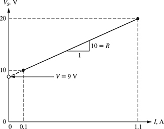
Figure 1.4 Voltage-current relationship for the data given in Fig. 1.3.
Using the data in Fig. 1.3, the slope m can be found as
![]()
Therefore, the current I can be written in slope-intercept form as
I = 0.1 Vs + b.
The y-intercept b can be determined using either one of the data points. Using the data point (Vs, I) = (10, 0.1) gives
0.1 = 0.1 (10) + b.
Solving for b gives
b = −0.9.
Therefore, the equation of the straight line can be written in the slope-intercept form as
Comparing equations (1.6) and (1.7) gives
![]()
and
![]()
Figure 1.5 is the graph of the straight line I = 0.1Vs − 0.9. Note that the y-intercept is ![]() A and the slope is
A and the slope is ![]() .
.
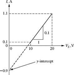
Figure 1.5 Straight line with I as independent variable for the data given in Fig. 1.3.
1.3 FORCE-DISPLACEMENT IN A PRELOADED TENSION SPRING
The force-displacement relationship for a spring with a preload fo is given by
where f is the force in Newtons (N), y is the displacement in meters (m), and k is the spring constant in N/m.

Figure 1.6 Force-displacement in a preloaded spring.
The objective is to find the spring constant k and the preload fo, if the values of the force and displacement are as given in Fig. 1.6.
Method 1 Treating the displacement y as an independent variable, the force-displacement relationship f = ky + fo is the equation of a straight line y = mx + b, where the independent variable x is the displacement y, the dependent variable y is the force f, the slope m is the spring constant k, and the y-intercept is the preload fo. The slope m can be calculated using the data given in Fig. 1.6 as
![]()
The equation of the force-displacement equation in the slope-intercept form can therefore be written as
f = 5y + b.
The y-intercept b can be found using one of the data points. Using the data point (f, y) = (5, 0.9) gives
5 = 5 (0.9) + b.
Solving for b gives
b = 0.5 N.
Therefore, the equation of the straight line can be written in slope-intercept form as
Comparing equations (1.8) and (1.9) gives
k = 5N/m, fo = 0.5N.
Method 2 Now treating the force f as an independent variable, the force-displacement relationship f = ky + fo can be written as ![]() . This relationship is the equation of a straight line y = mx + b, where the independent variable x is the force f, the dependent variable y is the displacement y, the slope m is the reciprocal of the spring constant
. This relationship is the equation of a straight line y = mx + b, where the independent variable x is the force f, the dependent variable y is the displacement y, the slope m is the reciprocal of the spring constant ![]() , and the y-intercept is the negated preload divided by the spring constant
, and the y-intercept is the negated preload divided by the spring constant ![]() . The slope m can be calculated using the data given in Fig. 1.6 as
. The slope m can be calculated using the data given in Fig. 1.6 as
![]()
The equation of the displacement y as a function of force f can therefore be written in slope-intercept form as
y = 0.2f + b.
The y-intercept b can be found using one of the data points. Using the data point (y, f) = (0.9, 5) gives
0.9 = 0.2 (5) + b.
Solving for b gives
b = −0.1.
Therefore, the equation of the straight line can be written in the slope-intercept form as
Comparing equation (1.10) with the expression ![]() gives
gives
![]()
and
![]()
Therefore, the force-displacement relationship for a preloaded spring given in Fig. 1.6 is given by
f = 5y + 0.5.
1.4 FURTHER EXAMPLES OF LINES IN ENGINEERING
The velocity of a vehicle follows the trajectory shown in Fig. 1.7. The vehicle starts at rest (zero velocity) and reaches a maximum velocity of 10 m/s in 2 s. It then cruises at a constant velocity of 10 m/s for 2 s before coming to rest at 6 s. Write the equation of the function v(t); in other words, write the expression of v(t) for times between 0 and 2 s, between 2 and 4 s, between 4 and 6 s, and greater than 6 s.

Solution
The velocity profile of the vehicle shown in Fig. 1.7 is a piecewise linear function with three different equations. The first linear function is a straight line passing through the origin starting at time 0 sec and ending at time equal to 2 s. The second linear function is a straight line with zero slope (cruise velocity of 10 m/s) starting at 2 s and ending at 4 s. Finally, the third piece of the trajectory is a straight line starting at 4 s and ending at 6 s. The equation of the piecewise linear function can be written as
(a) 0 ≤ t ≤ 2:
v(t) = mt + b
where b = 0 and ![]() . Therefore,
. Therefore,
v(t) = 5t m/s.
(b) 2 ≤ t ≤ 4:
v = 10 m/s.
(c) 4 ≤ t ≤ 6:
v(t) = mt + b,
where ![]() and the value of b can be calculated using the data point (t, v(t)) = (6, 0) as
and the value of b can be calculated using the data point (t, v(t)) = (6, 0) as
0 = −5 (6) + b ⇒ b = 0 + 30 = 30.
The value of b can also be calculated using the point-slope formula for the straight line
v − v1 = m(t − t1),
where v1 = 0 and t1 = 6. Thus,
v − 0 = −5(t − 6).
Therefore,
v(t) = −5(t − 6).
or
v(t) = −5t + 30 m/s.
(d) t > 6:
v(t) = 0 m/s.
The velocity of a vehicle is given in Fig. 1.8.
(a) Determine the equation of v(t) for
(i) 0 ≤ t ≤ 3 s
(ii) 3 ≤ t ≤ 6 s
(iii) 6 ≤ t ≤ 9 s
(iv) t ≥ 9
(b) Knowing that the acceleration of the vehicle is the slope of velocity, plot the acceleration of the vehicle.

(a) The velocity of the vehicle for different intervals can be calculated as
(i) 0 ≤ t ≤ 3 s:
v(t) = mt + b,
where ![]() and b = 24 m/s. Therefore,
and b = 24 m/s. Therefore,
v(t) = −4t + 24 m/s.
(ii) 3 ≤ t ≤ 6 s:
v(t) = 12 m/s.
(iii) 6 ≤ t ≤ 9 s:
v(t) = mt + b,
where ![]() and b can be calculated in slope-intercept form using point (t, v(t)) = (9, 0) as
and b can be calculated in slope-intercept form using point (t, v(t)) = (9, 0) as
0 = −4(9) + b.
Therefore, b = 36 m/s and
v(t) = −4t + 36 m/s.
(iv) t > 9 s:
v(t) = 0 m/s.
(b) Since the acceleration of the vehicle is the slope of the velocity in each interval, the acceleration a in m/s2 is given by
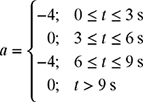
The plot of the acceleration is shown in Fig. 1.9.

Figure 1.9 Acceleration profile of the vehicle in Fig. 1.8.
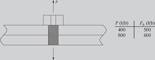
In a bolted connector shown in Fig. 1.10, the force in the bolt Fb is related to the external load P as
Fb = C P + Fi,
where C is the joint constant and Fi is the preload in the bolt.
(a) Determine the joint constant C and the preload Fi given the data in Fig. 1.10.
(b) Plot the bolt force Fb as a function of the external load P, and label C and Fi on the graph.
Solution
(a) The force-load relationship Fb = CP + Fi is the equation of a straight line, y = mx + b. The slope m is the joint constant C, which can be calculated as
![]()
Therefore,
Now, the y-intercept Fi can be calculated by substituting one of the data points into equation (1.11). Substituting the second data point (Fb, P) = (600, 800) gives
600 = 0.25 × 800 + Fi.
Solving for Fi yields
Fi = 600 − 200 = 400 lb.
Therefore, Fb = 0.25 P + 400 is the equation of the straight line, where C = 0.25 and Fi = 400 lb. Note that the joint constant C is dimensionless!
(b) The plot of the force Fb in the bolt as a function of the external load P is shown in Fig. 1.11.

Figure 1.11 Plot of the bolt force Fb as a function of the external load P.
For the electric circuit shown in Fig. 1.12, the relationship between the voltage V and the applied current I is given by V = (I + Io)R. Find the values of R and I0 if the voltage across the resistor V is known for the two different values of the current I as shown in Fig. 1.12.
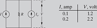
Figure 1.12 Circuit for Example 1-4.
Solution
The voltage-current relationship V = R I + R Io is the equation of a straight line y = mx + b, where the slope m = R can be found from the data given in Fig. 1.12 as
![]()
Therefore,
The y-intercept b = 10 I0 can be found by substituting the second data point (2.2, 0.2) in equation (1.12) as
2.2 = 100 × 0.2 + 10 I0.
Solving for I0 gives
10 I0 = 2.2 − 2 = 0.2,
I0 = 0.02 A.
Therefore, V = 10 I + 0.2; and R = 10 Ω and I0 = 0.02 A.
The output voltage vo of the operational amplifier (Op–Amp) circuit shown in Fig. 1.13 satisfies the relationship ![]() , where R in kΩ is the unknown resistance and vb is the unknown voltage. Fig. 1.13 gives the values of the output voltage for two different values of the input voltage.
, where R in kΩ is the unknown resistance and vb is the unknown voltage. Fig. 1.13 gives the values of the output voltage for two different values of the input voltage.
(a) Determine the value of R and vb.
(b) Plot the output voltage vo as a function of the input voltage vin. On the plot, clearly indicate the value of the output voltage when the input voltage is zero (y-intercept) and the value of the input voltage when the output voltage is zero (x-intercept).

Solution
(a) The input-output relationship ![]() is the equation of a straight line, y = mx + b, where the slope
is the equation of a straight line, y = mx + b, where the slope ![]() can be found from the data given in Fig. 1.13 as
can be found from the data given in Fig. 1.13 as
![]()
Solving for R gives R = 50 Ω. Therefore,

The y-intercept b = 3 vb can be found by substituting the first data point (v0, vin) = (5, 5) in equation (1.13) as
5 = −2 × 5 + 3 vb.
3 vb = 5 + 10 = 15,
which gives vb = 5 V. Therefore, vo = −2 vin + 15, R = 50 Ω, and vb = 5 V. The x-intercept can be found by substituting vo = 0 in the equation vo = −2 vin + 15 and finding the value of vin as
0 = −2 vin + 15,
which gives vin = 7.5 V. Therefore, the x-intercept occurs at Vin = 7.5 V.
(b) The plot of the output voltage of the Op–Amp as a function of the input voltage if vb = 5 V is shown in Fig. 1.14.

Figure 1.14 An Op–Amp circuit as a summing amplifier.
An actuator used in a prosthetic arm (Fig. 1.15) can produce a different amount of force by changing the voltage of the power supply. The force and voltage satisfy the linear relation F = kV, where V is the voltage applied and F is the force produced by the prosthetic arm. The maximum force the arm can produce is F = 44.5 N when supplied with V = 12 volts.
(a) Find the force produced by the actuator when supplied with V = 7.3 volts.
(b) What voltage is needed to achieve a force of F = 6.0 N?
(c) Using the results of parts (a) and (b), sketch the graph of F as a function of voltage V. Use the appropriate scales and clearly label the slope and the results of parts (a) and (b) on your graph.

(a) The input-output relationship F = kV is the equation of a straight line y = mx, where the slope m = k can be found from the given data as
![]()
Therefore, the equation of the straight line representing the actuator force F as a function of applied voltage V is given by
Thus, the force produced by the actuator when supplied with 7.3 volts is found by substituting V = 7.3 in equation (1.14) as
![]()
(b) The voltage needed to achieve a force of 6.0 N can be found by substituting F = 6.0 N in equation (1.14) as
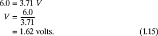
(c) The plot of force F as a function of voltage V can now be drawn as shown in Fig. 1.16.
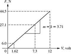
Figure 1.16 Plot of the actuator force verses the applied voltage.
The electrical activity of muscles can be monitored with an electromyogram (EMG). The following root mean square (RMS) value of the amplitude measurements of the EMG signal were taken when a woman was using her hand grip muscles to ensure a lid was tight on a jar.

Figure 1.17 Amplitude measurements of the EMG signal.
The RMS amplitude of the EMG signal satisfies the linear equation
where A is the RMS value of the EMG amplitude in V, F is the applied muscle force in N, and m is the slope.
(a) Determine the value of m and b.
(b) Plot the RMS amplitude A as a function of the applied muscle force F.
(c) Using the equation of the line from part (a), find the RMS value of the amplitude for a muscle force of 200 N.
Solution
(a) The input-output relationship A = mF + b is the equation of a straight line y = mx + b, where the slope m can be found from the EMG data given in the table (Fig. 1.17) as
![]()
The y-intercept b can be found by substituting the first data point (A, F) = (0.0005, 110) in equation (1.16) as
0.0005 = 4.55 × 10⁻⁶(110) + b.
Solving for b yields
b = 5 × 10⁻⁷ ≈ 0.
Therefore, the equation of the straight line representing the RMS amplitude as a function of applied force is given by
(b) The plot of the RMS amplitude as a function of the applied muscle force is shown in Fig. 1.18.

Figure 1.18 Plot of the RMS amplitude verses the applied muscle force.
(c) The RMS value of the amplitude for a muscle force of 200 N can be found by substituting F = 200 N in equation (1.17) as
A = 4.55 × 10−6 × (200) = 0.91 × 10⁻³V.
A civil engineer needs to establish the elevation of the cornerstone for a building located between two benchmarks, B1 and B2, of known elevations as shown in Fig. 1.19.
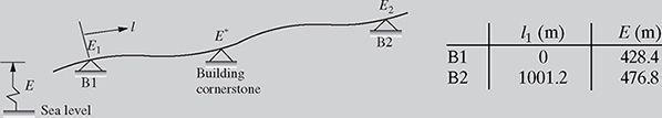
Figure 1.19 Elevations along a uniform grade.
The elevation E along the grade satisfies the linear relationship
where E1 is the elevation of B1, l is the distance from B1 along the grade, and m is the average slope of the grade.
(a) Find the equation of the line E and determine the slope m of the grade.
(b) Using the equation of the line from part (a), find the elevation of the cornerstone E* if it is located at a distance l = 565 m from B1.
(c) Sketch the graph of E as a function of l and clearly indicate both the slope m and elevation E1 of B1.
(a) The equation of elevation given by equation (1.18) is a straight line in the slope-intercept form y = mx + b, where the slope m can be found from the elevation data given in Fig. 1.19 as
![]()
The y-intercept E1 can be found by substituting the first data point (E, l) = (428.4, 0) in equation (1.18) as
428.4 = 0.0483 × (0) + E1
Solving for E1 yields
E1 = 428.4 m.
Therefore, the equation of the straight line representing the elevation as a function of distance l is given by
(b) The elevation E* of the cornerstone can be found by substituting l = 565 m in equation (1.19) as
E* = 0.0483 × (565) + 428.4 = 455.7 m.
(c) The plot of the elevation as a function of the length is shown in Fig. 1.20.

Figure 1.20 Elevation along a uniform grade.
PROBLEMS
-
1-1. A constant force F = 2 N is applied to a spring and the displacement x is measured as 0.2 m. If the spring force and displacement satisfy the linear relation F = kx, find the stiffness k of the spring.

-
1-2. The spring force F and displacement x for a close-wound tension spring are measured as shown in Fig. P1.2. The spring force F and displacement x satisfy the linear equation F = kx + Fi, where k is the spring constant and Fi is the preload induced during manufacturing of the spring.
(a) Using the given data in Fig. P1.2, find the equation of the line for the spring force F as a function of the displacement x, and determine the values of the spring constant k and preload Fi.
(b) Sketch the graph of F as a function of x. Use appropriate axis scales and clearly label the preload Fi, the spring constant k, and both given data points on your graph.

-
1-3. The spring force F and displacement x for a close-wound tension spring are measured as shown in Fig. P1.3. The spring force F and displacement x satisfy the linear equation F = kx + Fi, where k is the spring constant and Fi is the preload induced during manufacturing of the spring.
(a) Using the given data, find the equation of the line for the spring force F as a function of the displacement x, and determine the values of the spring constant k and preload Fi.
(b) Sketch the graph of F as a function of x and clearly indicate both the spring constant k and preload Fi.

-
1-4. In a bolted connection shown in Fig. P1.4, the force in the bolt Fb is given in terms of the external load P as Fb = CP + Fi.
(a) Given the data in Fig. P1.4, determine the joint constant C and the preload Fi.
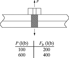
Figure P1.4 Bolted connection for problem P1-4.
(b) Plot the bolt force Fb as a function of the load P and label C and Fi on the graph.
-
1-5. Repeat problem P1-4 for the data given in Fig. P1.5.

-
1-6. The velocity v(t) of a ball thrown upward satisfies the equation v(t) = vo + at, where vo is the initial velocity of the ball in ft/s and a is the acceleration in ft/s2.
(a) Given the data in Fig. P1.6, find the equation of the line representing the velocity v(t) of the ball, and determine both the initial velocity vo and the acceleration a.
(b) Sketch the graph of the line v(t), and clearly indicate both the initial velocity and the acceleration on your graph. Also determine the time at which the velocity is zero.
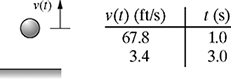
Figure P1.6 A ball thrown upward with an initial velocity vo(t) in problem P1-6.
-
1-7. The velocity v(t) of a ball thrown upward satisfies the equation v(t) = vo + at, where vo is the initial velocity of the ball in m/s and a is the acceleration in m/s2.
(a) Given the data in Fig. P1.7, find the equation of the line representing the velocity v(t) of the ball, and determine both the initial velocity vo and the acceleration a.
(b) Sketch the graph of the line v(t), and clearly indicate both the initial velocity and the acceleration on your graph. Also determine the time at which the velocity is zero.

Figure P1.7 A ball thrown upward with an initial velocity vo(t) in problem P1-7.
-
1-8. A model rocket is fired in the vertical plane. The velocity v(t) is measured as shown in Fig. P1.8. The velocity satisfies the equation v(t) = vo + at, where vo is the initial velocity of the rocket in m/s and a is the acceleration in m/s2.
(a) Given the data in Fig. P1.8, find the equation of the line representing the velocity v(t) of the rocket, and determine both the initial velocity vo and the acceleration a.
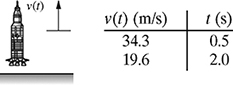
Figure P1.8 A model rocket fired in the vertical plane in problem P1-8.
(b) Sketch the graph of the line v(t) for 0 ≤ t ≤ 8 seconds, and clearly indicate both the initial velocity and the acceleration on your graph. Also determine the time at which the velocity is zero (i.e., the time required to reach the maximum height).
-
1-9. A model rocket is fired in the vertical plane. The velocity v(t) is measured as shown in Fig. P1.9. The velocity satisfies the equation v(t) = vo + at, where vo is the initial velocity of the rocket in ft/s and a is the acceleration in ft/s2.
(a) Given the data in Fig. P1.9, find the equation of the line representing the velocity v(t) of the rocket, and determine both the initial velocity vo and the acceleration a.
(b) Sketch the graph of the line v(t) for 0 ≤ t ≤ 10 seconds, and clearly indicate both the initial velocity and the acceleration on your graph. Also determine the time at which the velocity is zero (i.e., the time required to reach the maximum height).

Figure P1.9 A model rocket fired in the vertical plane in problem P1-9.
-
1-10. The velocity of a vehicle is measured at two distinct points in time as shown in Fig. P1.10. The velocity satisfies the relationship v(t) = vo + at, where vo is the initial velocity in m/s and a is the acceleration in m/s2.
(a) Find the equation of the line v(t), and determine both the initial velocity vo and the acceleration a.
(b) Sketch the graph of the line v(t), and clearly label the initial velocity, the acceleration, and the total stopping time on the graph.

Figure P1.10 Velocity of a vehicle during braking in problem P1-10.
-
1-11. The velocity of a vehicle is measured at two distinct points in time as shown in Fig. P1.11. The velocity satisfies the relationship v(t) = vo + at, where vo is the initial velocity in ft/s and a is the acceleration in ft/s2.
(a) Find the equation of the line v(t), and determine both the initial velocity vo and the acceleration a.
(b) Sketch the graph of the line v(t), and clearly label the initial velocity, the acceleration, and the total stopping time on the graph.
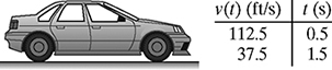
Figure P1.11 Velocity of a vehicle during braking in problem P1-11.
-
1-12. The velocity v(t) of a vehicle during braking is given in Fig. P1.12. Determine the equation for v(t) for
(a) 0 ≤ t ≤ 2 s
(b) 2 ≤ t ≤ 4 s
(c) 4 ≤ t ≤ 6 s
Figure P1.12 Velocity of a vehicle during braking in problem P1-12.
-
1-13. A linear trajectory is planned for a robot to pick up a part in a manufacturing process. The velocity of the trajectory of one of the joints is shown in Fig. P1.13. Determine the equation of v(t) for
(a) 0 ≤ t ≤ 1 s
(b) 1 ≤ t ≤ 3 s
(c) 3 ≤ t ≤ 4 s

-
1-14. The acceleration of the linear trajectory of problem P1-13 is shown in Fig. P1.14. Determine the equation of a(t) for
(a) 0 ≤ t ≤ 1 s
(b) 1 ≤ t ≤ 3 s
(c) 3 ≤ t ≤ 4 s

-
1-15. The temperature distribution in a well-insulated axial rod varies linearly with respect to distance when the temperature at both ends is held constant as shown in Fig. P1.15. The temperature satisfies the equation of a line T(x) = C1 x + C2, where C1 and C2 are constants of integration with units of °F/ft and °F, respectively
(a) Find the equation of the line T(x), and determine both constants C1 and C2.
(b) Sketch the graph of the line T(x) for 0 ≤ x ≤ 1.5 ft, and clearly label C1 and C2 on your graph. Also, clearly indicate the temperature at the center of the rod (x = 0.75 ft).
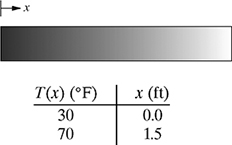
Figure P1.15 Temperature distribution in a well-insulated axial rod in problem P1-15.
-
1-16. The temperature distribution in a well-insulated axial rod varies linearly with respect to distance when the temperature at both ends is held constant as shown in Fig. P1.16. The temperature satisfies the equation of a line T(x) = C1 x + C2, where C1 and C2 are constants of integration with units of °C/m and °C, respectively.
(a) Find the equation of the line T(x), and determine both constants C1 and C2.
(b) Sketch the graph of the line T(x) for 0 ≤ x ≤ 0.5 m, and clearly label C1 and C2 on your graph. Also, clearly indicate the temperature at the center of the rod (x = 0.25 m).

Figure P1.16 Temperature distribution in a well-insulated axial rod in problem P1-16.
-
1-17. The voltage-current relationship for the circuit shown in Fig. P1.17 is given by Ohm's law as V = I R, where V is the applied voltage in volts, I is the current in amps, and R is the resistance of the resistor in ohms.
(a) Sketch the graph of I as a function of V if the resistance is 5 Ω.

Figure P1.17 Resistive circuit for problem P1-17.
(b) Find the current I if the applied voltage is 10 V.
-
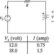
1-18. A voltage source Vs is used to apply two different voltages (12V and 18V) to the single-loop circuit shown in Fig. P1.18. The values of the measured current are shown in Fig. P1.18. The voltage and current satisfy the linear relation Vs = IR + V, where R is the resistance in ohms, I is the current in amps, and Vs is the voltage in volts.
(a) Using the data given in Fig. P1.18, find the equation of the line for Vs as a function of I, and determine the values of R and V.
(b) Sketch the graph of Vs as a function of I and clearly indicate the resistance R and voltage V on the graph.
-
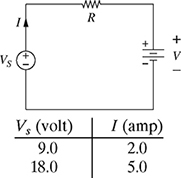
1-19. Repeat problem P1-18 for the data shown in Fig. P1.19.
-
1-20. Repeat problem P1-18 for the data shown in Fig. P1.20.

-
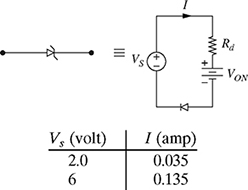
1-21. A linear model of a diode is shown in Fig. P1.21, where Rd is the forward resistance of the diode and VON is the voltage that turns the diode ON. To determine the resistance Rd and voltage VON, two voltage values are applied to the diode and the corresponding currents are measured. The applied voltage VS and the measured current I are given in Fig. P1.21. The applied voltage and the measured current satisfy the linear equation Vs = I Rd + VON.
(a) Find the equation of the line for Vs as a function of I and determine the resistance Rd and the voltage VON.

Figure P1.21 Linear model of a diode for problem P1-21.
(b) Sketch the graph of VS as a function of I, and clearly indicate the resistance Rd and the voltage VON on the graph.
-
1-22. Repeat problem P1-21 for the data given in Fig. P1.22.
-
1-23. The output voltage, vo, of the Op–Amp circuit shown in Fig. P1.23 satisfies the relationship

 , where R is the unknown resistance in kΩ and vb is the unknown voltage in volts. Fig. P1.23 gives the values of the output voltage for two different values of the input voltage.
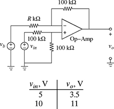
Figure P1.23 An Op–Amp circuit as a summing amplifier for problem P1.23.
(a) Determine the equation of the line for vo as a function of vin and find the values of R and vb.
(b) Plot the output voltage vo as a function of the input voltage vin. On the plot, clearly indicate the value of the output voltage when the input voltage is zero (y-intercept) and the value of the input voltage when the output voltage is zero (x-intercept).
-
1-24. The output voltage, vo, of the Op–Amp circuit shown in Fig. P1.24 satisfies the relationship
 , where R is the unknown resistance in kΩ, vin is the input voltage, and v2 is the unknown voltage. Fig. P1.24 gives the values of the output voltage for two different values of the input voltage vin.
(a) Find the equation of the line for vo as a function of vin and determine the values of R and v2.
(b) Plot the output voltage vo as a function of the input voltage vin. Clearly indicate the value of the output voltage when the input voltage is zero (y-intercept) and the value of the input voltage when the output voltage is zero (x-intercept).

-
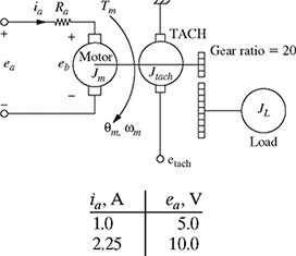
1-25. A DC motor is driving an inertial load JL shown in Fig. P1.25. To maintain a constant speed, two different values of the voltage ea are applied to the motor. The voltage ea and the current ia flowing through the armature winding of the motor satisfy the relationship ea = ia Ra + eb, where Ra is the resistance of the armature winding in ohms and eb is the back-emf in volts. Figure P1.25 gives the values of the current for two different values of the input voltage applied to the armature of the DC motor.
(a) Find the equation of the line for ea as a function of ia and determine the values of Ra and eb.
(b) Plot the applied voltage ea as a function of the current ia. Clearly indicate the value of the back-emf eb and the winding resistance Ra.

Figure P1.25 Voltage-current data of a DC motor for problem P1-25.
-
1-26. Repeat problem P1-25 for the data shown in Fig. P1.26.
Figure P1.26 Voltage-current data of a DC motor in problem P1-26.
-
1-27. In the active region, the output voltage vo of the n-channel enhancement-type MOSFET (NMOS) circuit shown in Fig. P1.27 satisfies the relationship vo = VDD − RD iD, where RD is the unknown drain resistance and VD is the unknown drain voltage. Fig. P1.27 gives the values of the output voltage for two different values of the drain current. Plot the output voltage vo as a function of the input drain current iD. On the plot, clearly indicate the values of RD and VDD.

-
1-28. Repeat problem P1-27 for the data given in Fig. P1.28.

-
1-29. An actuator used in a prosthetic arm can produce different amounts of force by changing the voltage of the power supply. The force and voltage satisfy the linear relation F = kV, where V is the voltage applied and F is the force produced by the prosthetic arm. The maximum force the arm can produce is 30.0 N when supplied with 10 V.
(a) Find the force produced by the actuator when supplied with 6.0 V.
(b) What voltage is needed to achieve a force of 5.0 N?
(c) Using the results of parts (a) and (b), sketch the graph of F as a function of voltage V. Use the appropriate scales and clearly label the slope and the results of parts (a) and (b).
-
1-30. The following two measurements of maximum heart rate R (in beats per minute, bpm) were recorded in an exercise physiology laboratory.
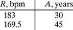
The maximum heart rate R and age A satisfy the linear equation
R = mA + B
where R is the heart rate in beats per minute and A is the age in years.
(a) Using the data provided, find the equation of the line for R.
(b) Sketch R as a function of A.
(c) Using the relationship developed in part (a), find the maximum heart rate of a 60-year-old person.
-
1-31. The electrical activity of muscles can be monitored with an electromyogram (EMG). The RMS amplitude measurements of the EMG signal when a person is using the hand grip muscle to tighten the lid on a jar is given in the table below:
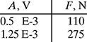
The RMS amplitude of the EMG signal satisfies the linear equation R = mA + B, where A is the RMS amplitude in volts, F is the applied muscle force in N, and m is the slope of the line.
(a) Using the data provided in the table, find the equation of the line for A(F).
(b) Sketch A as a function of F.
(c) Using the relationship developed in part (a), find the RMS amplitude for a muscle force of 200 N.
-
1-32. A civil engineer needs to establish the elevation of the cornerstone for a building located between two benchmarks, B1 and B2, of known elevations, as shown in Fig. P1.32.

Figure P1.32 Elevations along a uniform grade for exercise P1-32.
The elevation E along the grade satisfies the linear relationship

where E1 is the elevation of B1, l is the taped distance from B1 along the grade, and m is the rate of change of E with respect to l.
(a) Find the equation of the line E and determine the slope m of the linear relationship.
(b) Using the equation of the line from part (a), find the elevation of the cornerstone E* if it is located at a distance l = 300 m from B1.
(c) Sketch the graph of E as a function of l and clearly indicate both the slope m and elevation E1 of B1.
-
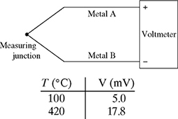
1-33. A thermocouple is a temperature measurement device, which produces a voltage V proportional to the temperature at the junction of two dissimilar metals. The voltage across a thermocouple is calibrated using the boiling point of water (100°C) and the freezing point of Zinc (420°C), as shown in Fig. P1.33.
Figure P1.33 Thermocouple to measure temperature in Celsius.
The junction temperature T and the voltage across the thermocouple V satisfy the linear equation
 , where α is the thermocouple sensitivity in mV/°C and TR is the reference temperature in °C.
(a) Using the calibration data given in Fig. P1.33, find the equation of the line for the measured temperature T as a function of the voltage V and determine the value of the sensitivity α and the reference temperature TR.
(b) Sketch the graph of T as a function of V and clearly indicate both the reference temperature TR and the sensitivity α on the graph.
-
1-34. The voltage across a thermocouple is calibrated using the boiling point of water (373°K) and the freezing point of Silver (1235°K), as shown in Fig. P1.34.
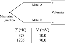
Figure P1.34 Thermocouple to measure temperature in Kelvin.
The junction temperature T and the voltage across the thermocouple V satisfy the linear equation
 , where α is the thermocouple sensitivity in mV/°K and TR is the reference temperature in °K.
(a) Using the calibration data given in Fig. P1.34, find the equation of the line for the measured temperature T as a function of the voltage V and determine the value of the sensitivity α and the reference temperature TR.
(b) Sketch the graph of T as a function of V and clearly indicate both the reference temperature TR and the sensitivity α on the graph.
-
1-35. An iron-costantan thermocouple is calibrated by inserting its junction in boiling water (100°C) and measuring a voltage V = 5.27 mV, and then inserting the juction in silver chloride at its melting point (455°C) and measuring V = 24.88 mV.
(a) Find the equation of the line for the measured temperature T as a function of the voltage V and determine the value of the sensitivity α and the reference temperature TR.
(b) Sketch the graph of T as a function of V and clearly indicate both the reference temperature TR and the sensitivity α on the graph.
(c) If the thermocouple is mounted in a chemical reactor and the voltage is observed to go from 10.0 mV to 13.6 mV, what is the change in temperature of the reactor?
-
1-36. Strain is a measure of the deformation of an object. It can be measured using a foil strain gauge shown in Fig. P1.36.
The strain being measured (
 ) and resistance of the sensor satisfy the linear equation
 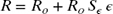 , where Ro is the initial resistance (measured in ohms, Ω) of the sensor with no strain, and
  is the gauge factor (a multiplier with NO units).
(a) Using the given data, find the equation of the line for the sensor's resistance R as a function of the strain
, and determine the values of the gauge factor and initial resistance Ro.(b) Sketch the graph of R as a function of
, and clearly indicate Ro on your graph.
Figure P1.36 Foil strain gauge to measure strain in problem P1-36.
-
1-37. Repeat problem P1-36 for the data shown in Fig. P1.37.
-
1-38. To determine the concentration of a purified protein sample, a graduate student used spectrophotometry to measure the absorbance given in the table below:

The concentration-absorbance relationship for this protein satisfies a linear equation a = mc + ai, where c is the concentration of a purified protein, a is the absorbance of the sample, m is the the rate of change of absorbance a with respect to concentration c, and ai is the y-intercept.

Figure P1.38 Foil strain gauge to measure strain in problem P1-38.
(a) Find the equation of the line that describes the concentration-absorbance relationship for this protein and determine the slope m of the linear relationship.
(b) Using the equation of the line from part (a), find the concentration of the sample if this sample had an absorption of 0.486.
(c) If the sample is diluted to a concentration of 0.00419 μg/ml, what would you expect the absorption to be? Would this value be accurate?
(d) Sketch the graph of absorbance a as a function of concentration c and clearly indicate both the slope m and the y-intercept.
-
1-39. Repeat problem P1-38 if the absorption-concentration data for another sample is obtained as

-
1-40. A chemistry student is performing an experiment to determine the temperature-volume behavior of a gas mixture at constant pressure and quantity. Due to technical difficulties, he could only obtain values at two temperatures as shown in the table below:
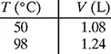
The student knows that the gas volume directly depends on temperature, that is, V(T) = mT + K, where V is the volume in L, T is the temperature in °C, K is the y-intercept in L, and m is the slope of the line in L/°C.
(a) Find the equation of the line that describes the temperature-volume relationship of the gas mixture and determine the slope m of the linear relationship.
(b) Using the equation of the line from part (a), find the temperature of the gas mixture if the volume is 1.15 L.
(c) Using the equation of the line from part (a), find the volume of the gas if the temperature is 70°C.
(d) Sketch the graph of the volume-temperature relationship for the gas mixture from −300°C to 100°C and clearly indicate both the slope m and the y-intercept. What is the significance of the temperature when V = 0 L?
-
1-41. To obtain the linear relationship between the Fahrenheit and Celsius temperature scales, the freezing and boiling point of water is used as given in the table below:
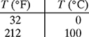
The relationship between the temperatures in Fahrenheit and Celsius scales satisfies the linear equation T (°F) = aT (°C) + b.
(a) Using the given data, find the equation of the line relating the Fahrenheit and Celsius scales.
(b) Sketch the graph of T (°F) as a function of T (°C), and clearly indicate a and b on your graph.
(c) Using the graph obtained in part (b), find the temperature interval in °C if the temperature is between 20°F and 80°F.
-
1-42. A thermostat control with dial marking from 0 to 100 is used to regulate the temperature of an oil bath. To calibrate the thermostat, the data for the temperature T (°F) versus the dial setting R was obtained as shown in the table below:

The relationship between the temperature T in Fahrenheit and the dial setting R satisfies the linear equation T (°F) = a R + b.
(a) Using the given data, find the equation of the line relating the temperature to the dial setting.
(b) Sketch the graph of T (°F) as a function of R, and clearly indicate a and b on your graph.
(c) Calculate the thermostat setting needed to obtain a temperature of 320°F.
-
1-43. In a pressure-fed journal bearing, forced cooling is provided by a pressurized lubricant flowing along the axial direction of the shaft (the x-direction) as shown in Fig. P1.43. The lubricant pressure satisfies the linear equation
 ,
,where ps is the supply pressure and l is the length of the bearing.
Figure P1.43 Pressure-fed journal bearing.
(a) Using the data given in the table (Fig. P1.43), find the equation of the line for the lubricant pressure p(x) and determine the values of the supply pressure ps and the bearing length l.
(b) Calculate the lubricant pressure p(x) if x is 1.0 in.
(c) Sketch the graph of the lubricant pressure p(x), and clearly indicate both the supply pressure ps and the bearing length l on the graph.