CHAPTER 7
HOW THE BUSINESS CYCLE CAN BE USED AS A ROAD MAP FOR INVESTING IN BONDS, STOCKS, AND COMMODITIES
The last chapter introduced us to the idea that the business cycle is continually repeating in a logical and sequential manner as some economic indicators, such as housing starts, lead the recovery and others, such as capital spending and the unemployment numbers, follow way behind. If we can pinpoint when a specific indicator has just turned and we know the direction of the trend of several others, we can use this whole framework as a road map to help us understand where we are in the business cycle and, more important, what is likely to happen next. The good news for investors is that the turning points of the three financial markets also form part of this sequential process. First bonds bottom, then stocks, and finally commodities. Then the whole process is repeated for the three peaks.
Armed with this knowledge of the chronological bond, stock, commodity sequence, we are able to create an actual financial map. We know there are three markets and that each one has two turning points—a top and a bottom—resulting in six turning points in each cycle. For the Smiths, it may be easiest to understand how financial assets relate to cycles by thinking in terms of the seasons of the calendar year.
The Seasonal Nature of the Business Cycle
Back in the early 1990s Martin Pring wrote a book titled The All-Season Investor (Wiley, 1992) in which he in part explained the repeating and sequential relationship between the different asset class performances in the business cycle. He referenced how the calendar year has four seasons, each of which has its own characteristics. The metaphor serves as an excellent way to better understand investing around a business cycle.
The Smiths enjoy their family vegetable garden and over the years take pride in planning, caring for, and reaping the rewards of their careful attention. They also understand that they need the right tools and knowledge to successfully manage the plot. In the spring, when the climate improves from the cold winter months, they till the soil and plant the seeds for the growing season. In the summer months the tending chores shift to weeding, watering, and fertilizing to nurture the crop along. In the fall, the reward for all the hard work is an abundant supply of fresh vegetables to enjoy and share with family and friends. Finally, the winter months are a time to relax, perhaps sharpen the garden tools, and prepare for the next planting season a few months away.
Like the seasons of the year, the environment for bonds, stocks, and commodities also changes in a repeatable and sequential fashion. The Smiths, like a majority of investors out there, are unaware of and unprepared for the ever-changing financial market seasons. Importantly, they are not even sure of the right tools to use to tend to their finances. Their gardening experience tells them that it is useless to plant in the winter when the snow is on the ground because it is not the right season to do this. Planting seeds when it is too cold for them to germinate makes no agricultural sense at all. The same is true for the financial seasons in the business cycle. By better understanding these financial seasons and using the correct tools, the Smiths can make well-informed decisions and dramatically improve their chances for investment success.
Indeed, investors can use knowledge of the chronological bond, stock, and commodity sequence to create an actual financial map. We like to refer to the components as the three main food groups: bonds, stocks, and commodities or inflation-sensitive investments. Each one has two turning points in a given business cycle—a top and a bottom. This means that a typical cycle has six turning points—buy and sell for each of the three asset classes. We call these the six stages. The calendar year has four seasons, each of which has its own characteristics. The same can be said for the typical four- to five-year business cycle, which has six stages. We will explain the important historical features of each stage and how understanding the sequence can be invaluable to the successful rotation of assets.
In this chapter we describe the various stages, together with some of their broader implications for investment. Later on the discussion will turn to the more practical subject of how these stages may be identified as well as a description of the indicators to help you accomplish this task.
The Six Stages
The six stages of the business cycle are illustrated in Figure 7-1. The cycle begins with bonds in a bottoming mode and continues all the way through until the eventual peak in commodity prices.
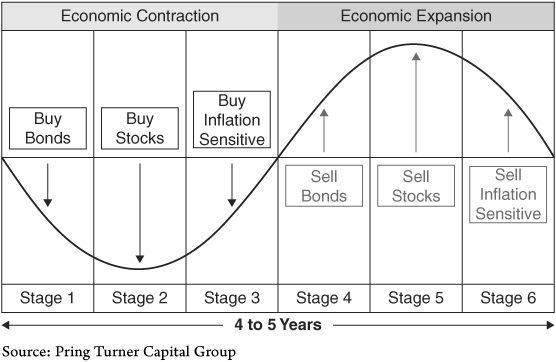
FIGURE 7-1 Pring Turner’s Six Business Cycle Stages
Follow the business cycle sequence to dynamically adjust asset allocations and emphasize or deemphasize each asset class for optimal risk-adjusted returns.
The figure shows an idealized situation that does not necessarily develop exactly according to plan in the real world. To start with, it implies that each stage is equal in duration, but in reality this is not the case. Occasionally two markets may reverse simultaneously. This is what happened in October 1966 when both bonds and stocks bottomed together. In such a situation the cycle moves from stage 6, when all three markets are declining, directly to stage 2 where bonds and stocks are bullish and commodities bearish. Stage 1, in which bonds are bullish and the other two markets are bearish, is therefore bypassed. On the other hand, there was an almost two-year lag between the 1984 low in stocks and the 1986 bottom in commodities.
It is not unprecedented for the markets themselves to reverse direction out of sequence. Commodities bottomed ahead of stocks in 1937. This turned out to be an unusually bullish situation since it represented the early years of a multidecade rise in commodity prices. While not normal, it nonetheless serves as a reminder that the sequential approach described here is by no means automatic. If it worked like clockwork in every cycle, everyone would be using this approach and it would be instantly discounted. Our research indicates that the six stages move sequentially approximately 85 percent of the time. This knowledge is an enormous edge for investors. These concepts should therefore be used as an overall basis for analysis and investment policy, but not to the total exclusion of independent thinking. The rest of this chapter is devoted to a description of the kind of investment environment that can be expected at each stage. Afterward we will be in a position to look at some ways in which the stages can be identified.
A General Overview
Figure 7-2 shows the bell-shaped curves for the three asset classes (bonds, stocks, and commodities). Since each one dances to the beat of a different drummer in the business cycle, there are times when they are moving in different trajectories and times when they are all operating in the same direction. The two highlighted boxes indicate periods when all three markets are either rising or falling simultaneously—stages 3 and 6, respectively.
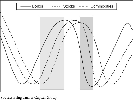
FIGURE 7-2 Theoretical Bell Curves for Bonds, Stocks, and Commodities
The three asset classes move in different trajectories during the typical business cycle. The shaded boxes indicate periods when all three markets are either rising or falling simultaneously. The rest of the time they tend to move in different trajectories.
Figure 7-3 demonstrates when the various assets should be emphasized. This is shown in the shaded boxes at the bottom of the diagram.
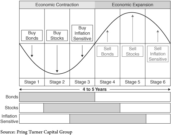
FIGURE 7-3 Pring Turner’s Six Business Cycle Stages
The six-stage model can help investors dynamically adjust asset allocations around the typical business cycle sequence. Essentially an investor needs two game plans: one for defense to protect assets in difficult periods and one for offense to grow wealth during favorable conditions.
To review, the bell-shaped curve represents the ebbs and flows of business activity in the four- to five-year cycle. The left side starts with the economy in recession and is the starting point for our model. At this time bondholders have everything on their side. First, credit demand is falling like a stone because of the lackluster economy; businesses are battening down the hatches and paying down, not expanding debt. Second, the Fed is now committed to fighting the unemployment battle and is pumping money into the banking system as fast as it can. This falling demand and expanding supply of credit reduces its price (interest rates). Since bond prices move inversely with interest rates, this means that good-quality bonds will appreciate in value. From a risk versus reward standpoint stage 1 is generally good for bonds but not as kind to stocks and commodities.
Next, in the depths of recession and after interest rates have declined and bond prices appreciated, the stock market begins to turn up. This point befuddles most investors because the stock market begins a dynamic cyclical advance when the economic news cannot be any worse. A stock market bottom by definition is the point of maximum pessimism. Knowledgeable investors take advantage of the stock market’s character to be one of the most dependable leading economic indicators. It still takes courage (and cash) to buy stock in the midst of miserable economic headlines. This is typical behavior for stage 2 where stocks start to show strong performance. At this point two asset classes are in cyclical bull markets, bonds and stocks, while commodities are still underperforming. As the economy picks up steam, the demand for raw materials increases, and finally commodity prices join the party. This is distinctive of a stage 3 environment, where all three asset classes are doing well, and everyone, including the Smiths, are investment geniuses.
Eventually, we have too much of a good thing as the economy and commodity prices heat up and inflationary forces take hold. This development gets the attention of the Federal Reserve. Taking its cue from rising inflation, the Fed begins the process of tightening monetary conditions and starts to raise interest rates for this cycle. This action immediately affects bond prices negatively and signals the typical stage 4 where bonds do poorly, but stocks and commodities continue to rally. When rates move high enough, the stock market eventually takes notice and prices turn down in anticipation of an oncoming economic slowdown. Stage 5 is now positive only for commodities, as bonds and stocks begin their cyclical declines. Finally, sagging demand for resources resulting from the slowing economy pushes commodities into their cyclical downturn, and now in stage 6 all three asset classes are in bear markets. The cycle is complete, and the next step is to anticipate the move back to stage 1 for a repeat of the process.
Some of you more observant readers may be asking about any other possible combinations that may fall outside the theoretical six-stage model. In fact, there are two other potential scenarios to look for when the asset classes get out of sequence. This happens when bonds and commodities are bearish leaving stocks bullish, and when bonds and commodities are bullish and stocks are bearish. We refer to these as stages 7 and 8 and acknowledge that while these two do not happen very often (about 10 percent of the time), they certainly need to be taken into consideration.
When you think about it, the cycle can really be split into two parts—an inflationary part and a deflationary one. This is shown in Figure 7-4, where the vertical partition serves as a rough guide for asset allocation. During the deflationary stage, bonds and defensive and high-dividend stocks would be appropriate. However, in the inflationary stage exposure to commodity ETFs, resource-based and basic industry stocks, and so on make more sense.

FIGURE 7-4 Deflationary and Inflationary Parts of the Business Cycle
During the deflationary stage, bonds and defensive high-dividend stocks are appropriate. The inflationary stage should emphasize commodity ETFs or resource-based and basic industry stocks.
Now that we have outlined this rather stark contrast between the basic dual phases of the cycle, it makes sense to discuss some rudimentary aspects of asset allocation around the stages. The material covered in this chapter is general in nature but don’t worry. If you want to drill down more on this subject, we have included a more detailed account in Appendix D.
Applying Business Cycle Stage Shifts to Asset Allocation Changes
The key point in applying cycle stage shifts to changes in asset allocation is viewing asset allocation within the context of understanding the risk and reward characteristics of the different asset classes at each stage of the economic cycle. (See Table 7-1.)

TABLE 7-1 Broad Business Cycle Asset Allocation Guidelines
This broad asset allocation guideline can serve as an important starting point for actively managing portfolios throughout the business cycle.
For instance, during a recession in stage 1 the allocation includes a healthy mix of bonds and cash to stabilize portfolio values. The opposite is true in stage 3, when the economy is running at full throttle and maximum exposure to stocks is recommended. Doesn’t it make sense to reduce exposure to stocks in anticipation of a recession and to reemphasize them just prior to when the economy is expected to accelerate into a growth mode? In this sense important asset allocation decisions are not static rules based solely on your age and risk temperament. Instead, asset levels should be actively changed based on the historical risk/reward relationship of each level around the normal cyclical swings in the economy and financial markets. We believe that our six-stage framework is an ideal way to construct an active allocation discipline, especially because it also serves as a critical risk-management tool.
However, it is important to remember that no strategy or discipline is perfect and that each has its own shortcomings. In the case of economic fluctuations, not all cycles will experience every stage, and stages occasionally diverge from the expected sequential order. Sometimes the cycle will skip a stage or even two. In fact a cycle may also retrograde to a previous phase. Another drawback is that a lot of specific stages will be identified only after they have been under way for some time. These are additional reasons why changes to portfolio allocations should be gradual. You should take into account other considerations, including market action itself. Finally, larger allocation switches can be justified only when the evidence of a change in the environment is overwhelming and markets have not already gone too far in factoring this into prices. Nonetheless, over several decades the investment management team at Pring Turner Capital Group has found the methodology to be an invaluable tool in successfully managing client portfolios while taking less overall market risk. For investors, the beauty of following the repetitious nature of the business cycle is an investment methodology that never goes out of style.
In the next chapter we will further study the historical performance data of stocks, bonds, and commodities and give you more tools to help you use the business cycle to your best advantage. We will explain a “quick test” to help you easily identify what stage of the cycle we are in. Going a step further, we will also share invaluable sector performance data around the stages that can help you detect the best and worst sectors for each stage of the business cycle. Sector emphasis around the cycle is an additional risk-management tool to drive even better performance while reducing risk.
KEY POINTS
1. We organize the business cycle into six stages to identify which asset class to favor or underweight in each stage.
2. During secular bear markets, the economy is often in recession, and business cycle analysis has added importance.
3. Optimal asset allocation for portfolios can be adjusted based on the business cycle stage in an effort to increase returns and reduce risks.
IMPORTANT QUESTIONS FROM THE SMITHS
We see that the average business cycle lasts between four and five years, yet between 1990 and 2001 there was no recession. Doesn’t this question the validity of your thesis?
That is a great question. First, that period developed for the most part under the context of a secular bull market where recessions are shallow and far less common. Second, even during these long patches between recessions, the economic growth path slows down every four years or so. The difference is that growth slows, but it does not contract. We still get the bond and stock commodity sequence, but the difference is that equities avoid a full-fledged bear market. In 1994, for example, the average stock lost about 20 percent, and the market experienced a sideways trading range, not an extended decline as it probably would have experienced if a recession had emerged. Compare that to the 2008–2009 period when the economy declined sharply as did the stock market.
The business cycle research relating to the U.S. economy makes sense, but the rest of the world does not just revolve around the United States. Is your work still relevant as the global economy becomes more interconnected? How do you take advantage of growth outside the United States?
Your observation may be true to some extent, but the United States is still the largest economy in the world with significant corporate revenues being generated by overseas operations. Indeed, many of the largest companies in the United States have a greater contribution of sales from global markets than within our borders. Companies like Caterpillar, Coca-Cola, Intel, and Procter & Gamble are just a few of the global growth beneficiaries based in the United States. The important point is that just because we expect the U.S. economy to face headwinds in the second lost decade, global leadership companies are still likely to continue to see rising profits. Fortunately, you are able to invest in companies, not economies. In essence, global economies are tracking each other in a more correlated manner than ever before, and following the U.S. business cycle remains as important as ever. It is also quite evident that parts of the world are growing much faster than others. In very broad terms we can segregate those in secular bull markets from those in secular bears.
Many of the economies in the developed world are in secular bear markets and have been since 2000. This includes the United States, Western Europe, and Japan, whose economies share certain negative common characteristics—high debt, slow growth, aging populations, and persistent high unemployment. On the other hand, the economies experiencing secular bull behavior include the emerging economies in Asia, Latin America, and Eastern Europe. These developing countries have certain positive common characteristics—low debt, high growth, young populations, and strong job markets. In addition, a few resource-based developed countries like Canada, Australia, and South Africa offer opportunities to invest in areas that benefit from the continued infrastructure build-out taking place in the developing world.
From an investment standpoint there are some distinctions to make and considerations for portfolio managers. While the emerging markets show the highest growth potential, they have also exhibited the highest level of volatility. It is not unusual to find these markets with volatility readings (beta and standard deviations for instance) at 40 to 50 percent higher levels than the U.S. market. They exemplify the investment adage: higher risks for higher return potential. For example, when the U.S. markets drop by 20 percent, these high beta markets can decline by 30 percent or more. For conservative investors, this may be a bit more excitement than they bargained for. One solution is to take smaller bites for portfolio allocation purposes with the idea that a little bit can go a long way. Another suggestion is to view the investments as “tactical” buys for a shorter-term holding period. For instance, you may consider allocating 8 percent of a portfolio to Asian emerging markets. Then after you see them advance, you can trim the position back to 4 percent or even less. After an intermediate decline, the position can be fully established once again for the next intermediate up move. This viable tactic is called “trading around the core”—where a long-term “core” investment position is kept in a favorable secular bull market asset, but a tactical trading position is managed around the intermediate term (two to six months) and is especially important around the cyclical (four to five years) moves.
The key observation is that there are opportunities around the globe and within the United States for leading beneficiaries of the dynamic global growth occurring in emerging economies. Many U.S.-based companies offer a safer way to profit from this growth while sporting consistent earnings and dividend histories. Additionally, direct investments in emerging markets have to be made with caution and the understanding that they can be substantially more volatile than the U.S. markets. At Pring Turner Capital Group we prefer using these markets as tactical plays where we move in and out based on our market outlook for each and the comparative relative strength characteristics versus the U.S. market.