Sub-sequences, Regions, Runs, Gaps, and Islands
Abstract
The groups in a GROUP BY do not depend on any orderings. But you will often want to make other groupings which depend on an ordering of some kind. Examples of this sort of data would be ticket numbers, time series data taken at fixed intervals, and the like which can have missing data or sub-sequences that are of interest.
We have already talked about the GROUP BY clause in queries. The groups in a GROUP BY do not depend on any orderings. But you will often want to make other groupings which depend on an ordering of some kind. Examples of this sort of data would be ticket numbers, time series data taken at fixed intervals, and the like which can have missing data or sub-sequences that are of interest. These things are easier to explain with examples. Consider a skeleton table with a sequential key and seven rows.
CREATE TABLE List
(list_seq INTEGER NOT NULL PRIMARY KEY,
list_val INTEGER NOT NULL UNIQUE);
INSERT INTO List
VALUES (1, 99), (2, 10), (3, 11), (4, 12), (5, 13), (6, 14), (7, 0);
A sub-sequence in the list_val column can be increasing, decreasing, monotonic, or not. Let’s look at rows where the values are increasing uniformly by steps of one. You can find sub-sequences of size three which follow the rule—(10, 11, 12), (11, 12, 13), and (12, 13, 14)—but the longest sub-sequence is (10, 11, 12, 13, 14) and it is of size five.
A run is like a sequence, but the numbers do not have to be consecutive, just increasing (or decreasing) and in sequence. For example, given the run {(1, 1), (2, 2), (3, 12), (4, 15), (5, 23)}, you can find sub-runs of size three: (1, 2, 12), (2, 12, 15), and (12, 15, 23).
A region is contiguous and all the values are the same. For example, {(1, 1), (2, 0), (3, 0), (4, 0), (5, 25)} has a region of zeros that is three items long.
In procedural languages, you would simply sort the data and scan it. In SQL, you used to have to define everything in terms of sets and fancy joins to get an ordering if it was not in the data. Today, we have ROW_NUMBER() to get us a sequence number for ordering the data.
32.1 Finding Subregions of Size (n)
This example is adapted from SQL and its applications (Lorie and Daudenarde, 1991).1 You are given a table of theater seats, defined by
CREATE TABLE Theater
(seat_nbr INTEGER NOT NULL PRIMARY KEY, -- sequence
occupancy_status CHAR(1) DEFAULT 'A' NOT NULL -- values
CONSTRAINT valid_occupancy_status
CHECK (occupancy_status IN ('A', 'S'));
where an occupancy_status code of ‘A’ means available and ‘S’ means sold. Your problem is to write a query that will return the subregions of (n) consecutive seats still available. Assume that consecutive seat numbers mean that the seats are also consecutive for a moment, ignoring rows of seating where seat_nbr(n) and seat_nbr((n) + 1) might be on different physical theater rows. For (n) = 3, we can write a self-JOIN query, thus:
SELECT T1.seat_nbr, T2.seat_nbr, T3.seat_nbr
FROM Theater AT T1, Theater AT T2, Theater AT T3
WHERE T1.occupancy_status = 'A'
AND T2.occupancy_status = 'A'
AND T3.occupancy_status = 'A'
AND T2.seat_nbr = T1.seat_nbr + 1
AND T3.seat_nbr = T2.seat_nbr + 1;
The trouble with this answer is that it works only for (n = 3) and for nothing else. This pattern can be extended for any (n), but what we really want is a generalized query where we can use (n) as a parameter to the query.
The solution given by Lorie and Daudenarde starts with a given seat_nbr and looks at all the available seats between it and ((n) − 1) seats further up. The real trick is switching from the English-language statement “All seats between here and there are available” to the passive-voice version, “Available is the occupancy_status of all the seats between here and there”, so that you can see the query.
SELECT seat_nbr, ' thru ', (seat_nbr + (:n - 1))
FROM Theater AS T1
WHERE occupancy_status = 'A'
AND 'A' = ALL (SELECT occupancy_status
FROM Theater AS T2
 WHERE T2.seat_nbr > T1.seat_nbr
 AND T2.seat_nbr <= T1.seat_nbr + (:n - 1));
Please notice that this returns subregions. That is, if seats (1, 2, 3, 4, 5) are available, this query will return (1, 2, 3), (2, 3, 4), and (3, 4, 5) as its result set.
32.2 Numbering Regions
Instead of looking for a region, we want to number the regions in the order in which they appear. For example, given a view or table with a payment history we want to break it into grouping of behavior, say whether or not the payments were on time or late. This is a bad design; we should use a NULL-able payment date, but this is easier to read.
CREATE TABLE Payment_History
(payment_nbr INTEGER NOT NULL PRIMARY KEY,
paid:on_time_flg CHAR(1) DEFAULT 'Y' NOT NULL
CHECK(paid:on_time_flg IN ('Y', 'N')));
INSERT INTO Payment_History
VALUES (1006, 'Y'), (1005, 'Y'), (1004, 'N'),
(1003, 'Y'), (1002, 'Y'), (1001, 'Y'),
(1000, 'N'),
The results we want assign a grouping number to each run of on-time/late payments, thus
A solution by Hugo Kornelis depends on the payments always being numbered consecutively. Today we can guarantee this by using a CREATE SEQUENCE statement for each account.
SELECT (SELECT COUNT(*)
 FROM Payment_History AS H2,
 Payment_History AS H3
 WHERE H3.payment_nbr = H2.payment_nbr + 1
AND H3.paid:on_time_flg <> H2.paid:on_time_flg
AND H2.payment_nbr >= H1.payment_nbr) + 1 AS grping,
 payment_nbr, paid:on_time_flg
FROM Payment_History AS H1;
This can be modified for more types of behavior. This is not a modern SQL idiom and will not perform as well as the ordinal functions. But you need to know it to replace it. Let’s assume we have a test that returns ‘A’ or ‘B’ and we want to see clusters where the score stayed the same:
CREATE TABLE Tests
(sample_time DATE NOT NULL PRIMARY KEY,
  sample_score CHAR(1) NOT NULL);
INSERT INTO Tests
VALUES ('2018-01-01', 'A'),
('2018-01-02', 'A'),
('2018-01-03', 'A'),
('2018-01-04', 'B'),
('2018-01-05', 'B'),
('2018-01-06', 'A'),
('2018-01-07', 'A'),
('2018-01-08', 'A'),
('2018-01-09', 'A'),
('2018-01-10', 'B'),
('2018-01-11', 'B'),
('2018-01-12', 'A'),
('2018-01-13', 'A'),
('2018-01-14', 'C'),
('2018-01-15', 'D'),
('2018-01-16', 'A'),
SELECT MIN(X.sample_time) AS cluster_start,
MAX(X.sample_time) AS cluster_end,
MIN(X.sample_score) AS cluster_score
FROM (SELECT sample_time, sample_score,
(ROW_NUMBER () OVER (ORDER BY sample_time)
- ROW_NUMBER() OVER (PARTITION BY sample_score
ORDER BY sample_time))
FROM Tests) AS X(sample_time, sample_score, cluster_nbr)
GROUP BY cluster_nbr;
| cluster_start | cluster_end | cluster_score |
| ‘2014-01-01’ | ‘2014-01-03’ | A |
| ‘2014-01-04’ | ‘2014-01-05’ | B |
| ‘2014-01-06’ | ‘2014-01-09’ | A |
| ‘2014-01-10’ | ‘2014-01-11’ | B |
| ‘2014-01-12’ | ‘2014-01-13’ | A |
| ‘2014-01-14’ | ‘2014-01-14’ | C |
| ‘2014-01-15’ | ‘2014-01-15’ | D |
| ‘2014-01-16’ | ‘2014-01-16’ | A |
These groupings are called clusters or islands or “OLAP sorting” in the literature.
32.3 Finding Regions of Maximum Size
A query to find a region, rather than a subregion of a known size, of seats was presented in SQL Forum (Rozenshtein, Abramovich, and Birger, 1997).2
SELECT T1.seat_nbr AS start_seat_nbr, T2.seat_nbr AS end_seat_nbr
FROM Theater AS T1, Theater AS T2
WHERE T1.seat_nbr < T2.seat_nbr
AND NOT EXISTS
(SELECT *
 FROM Theater AS T3
 WHERE (T3.seat_nbr BETWEEN T1.seat_nbr AND T2.seat_nbr
AND T3.occupancy_status <> 'A')
 OR (T3.seat_nbr = T2.seat_nbr + 1
AND T3.occupancy_status = 'A')
 OR (T3.seat_nbr = T1.seat_nbr - 1
AND T3.occupancy_status = 'A'));
The trick here is to look for the starting and ending seats in the region. The starting seat_nbr of a region is to the right of a sold seat_nbr and the ending seat_nbr is to the left of a sold seat. No seat between the start and the end has been sold.
If you only keep the available seat_nbrs in a table, the solution is a bit easier. It is also a more general problem that applies to any table of sequential, possibly noncontiguous, data
CREATE TABLE Available_Seating
(seat_nbr INTEGER NOT NULL
CONSTRAINT valid_seat_nbr
CHECK (seat_nbr BETWEEN 001 AND 999));
INSERT INTO Seatings
VALUES (199), (200), (201), (202), (204),
(210), (211), (212), (214), (218);
where you need to create a result which will show the start and finish values of each sequence in the table, thus:
This is a common way of finding the missing values in a sequence of tickets sold, unaccounted for invoices and so forth. Imagine a number line with closed dots for the numbers that are in the table and open dots for the numbers that are not. What you see about a sequence? Well, we can start with a fact that anyone who has done inventory knows. The number of elements in a sequence is equal to the ending sequence number minus the starting sequence number plus one. This is a basic property of ordinal numbers:
(finish − start + 1) = count of open seats
This tells us that we need to have a self-JOIN with two copies of the table, one for the starting value and one for the ending value of each sequence. Once we have those two items, we can compute the length with our formula and see if it is equal to the count of the items between the start and finish.
SELECT S1.seat_nbr, MAX(S2.seat_nbr) -- start and rightmost item
FROM AvailableSeating AS S1
INNER JOIN
AvailableSeating AS S2 -- self-join
 ON S1.seat_nbr <= S2.seat_nbr
 AND (S2.seat_nbr - S1.seat_nbr + 1) -- formula for length
= (SELECT COUNT(*) -- items in the sequence
FROM AvailableSeating AS S3
 WHERE S3.seat_nbr BETWEEN S1.seat_nbr
 AND S2.seat_nbr)
AND NOT EXISTS (SELECT *
FROM AvailableSeating AS S4
 WHERE S1.seat_nbr - 1
= S4.seat_nbr)
GROUP BY S1.seat_nbr;
Finally, we need to be sure that we have the furthest item to the right as the end item. Each sequence of (n) items has (n) sub-sequences that all start with the same item. So we finally do a GROUP BY on the starting item and use a MAX() to get the rightmost value.
However, there is a faster version with three tables. This solution is based on another property of the longest possible sequences. If you look to the right of the last item, you do not find anything. Likewise, if you look to the left of the first item, you do not find anything either. These missing items that are “just over the border” define a sequence by framing it. There also cannot be any “gaps”—missing items—inside those borders. That translates into SQL as:
SELECT S1.seat_nbr, MIN(S2.seat_nbr) -- start and leftmost border
FROM AvailableSeating AS S1, AvailableSeating AS S2
WHERE S1.seat_nbr <= S2.seat_nbr
AND NOT EXISTS -- border items of the sequence
(SELECT *
 FROM AvailableSeating AS S3
 WHERE S3.seat_nbr NOT BETWEEN S1.seat_nbr AND S2.seat_nbr
 AND (S3.seat_nbr = S1.seat_nbr - 1
OR S3.seat_nbr = S2.seat_nbr + 1))
GROUP BY S1.seat_nbr;
The leftmost and rightmost members of the block of seats are found by looking for the status of the seats just over the boundary. Once we have the rightmost seat the block and then we can do a GROUP BY and MIN() to get what we want.
Since the second approach uses only three copies of the original table, it should be a bit faster. Also, the EXISTS() predicates can often take advantage of indexing and thus run faster than subquery expressions which require a table scan.
The new ordinal functions allow you to answer these queries without explicit self-joins or a sequencing column. Since self-joins are expensive, it is better to use ordinal functions that might be optimized. Consider a single column of integers:
CREATE TABLE Foobar (data_val INTEGER NOT NULL PRIMARY KEY);
INSERT INTO Foobar
VALUES (1), (2), (5), (6), (7), (8), (9), (11), (12), (22);
Here is a query to get the final results:
WITH X (data_val, data_seq, absent_data_grp)
AS
(SELECT data_val,
ROW_NUMBER() OVER (ORDER BY data_val ASC) ,
(data_val
 - ROW_NUMBER() OVER (ORDER BY data_val ASC))
FROM Foobar)
SELECT absent_data_val, COUNT(*), MIN(data_val) AS start_data_val
FROM X
GROUP BY absent_data_val;
The CTE produces this result. The absent_data_grp tells you how many values are missing from the data values, just not what they are.
The final query gives us:
So, the maximum contiguous sequence is five rows. Since it starts at 5, we know that the contiguous set is {5, 6, 7, 8, 9}.
32.4 Bound Queries
Another form of query asks if there was an overall trend between two points in time bounded by a low value and a high value in the sequence of data. This is easier to show with an example. Let us assume that we have data on the selling prices of a stock in a table. We want to find periods of time when the price was generally increasing. Consider this data:
The stock was generally increasing in all the periods that began on December 1 or ended on December 5—that is, it finished higher at the ends of those periods, in spite of the slump in the middle. A query for this problem is
SELECT S1.sale_date AS start_date, S2.sale_date AS finish_date
FROM MyStock AS S1, MyStock AS S2
WHERE S1.sale_date < S2.sale_date
AND NOT EXISTS
(SELECT *
FROM MyStock AS S3
 WHERE S3.sale_date BETWEEN S1.sale_date AND S2.sale_date
AND S3.stock_price
 NOT BETWEEN S1.stock_price AND S2.stock_price);
32.5 Run and Sequence Queries
Runs are informally defined as sequences with gaps. That is, we have a set of unique numbers whose order has some meaning, but the numbers are not all consecutive. Time series information where the samples are taken at irregular intervals is an example of this sort of data. Runs can be constructed in the same manner as the sequences by making a minor change in the search condition. Let’s do these queries with an abstract table made up of a sequence number and a value:
CREATE TABLE Runs
(list_seq INTEGER NOT NULL PRIMARY KEY,
list_val INTEGER NOT NULL);
Runs
| list_seq | list_val |
| 1 | 6 |
| 2 | 41 |
| 3 | 12 |
| 4 | 51 |
| 5 | 21 |
| 6 | 70 |
| 7 | 79 |
| 8 | 62 |
| 9 | 30 |
| 10 | 31 |
| 11 | 32 |
| 12 | 34 |
| 13 | 35 |
| 14 | 57 |
| 15 | 19 |
| 16 | 84 |
| 17 | 80 |
| 18 | 90 |
| 19 | 63 |
| 20 | 53 |
| 21 | 3 |
| 22 | 59 |
| 23 | 69 |
| 24 | 27 |
| 25 | 33 |
One of the problems is that we do not want to get back all the runs and sequences of length one. Ideally, the length (n) of the run should be adjustable. This query will find runs of length (n) or greater; if you want runs of exactly (n), change the “greater than” to an equal sign.
SELECT R1.list_seq AS start_list_seq,
R2.list_seq AS end_list_seq_nbr
FROM Runs AS R1, Runs AS R2
 WHERE R1.list_seq < R2.list_seq -- start and end points
 AND (R2.list_seq - R1.list_seq) > (:n - 1) -- length restrictions
 AND NOT EXISTS -- ordering within the end points
(SELECT *
 FROM Runs AS R3, Runs AS R4
 WHERE R4.list_seq BETWEEN R1.list_seq AND R2.list_seq
 AND R3.list_seq BETWEEN R1.list_seq AND R2.list_seq
 AND R3.list_seq < R4.list_seq
 AND R3.list_val > R4.list_val);
What this query does is set up the S1 sequence number as the starting point and the S2 sequence number as the ending point of the run. The monster subquery in the NOT EXISTS() predicate is looking for a row in the middle of the run that violates the ordering of the run. If there is none, the run is valid. The best way to understand what is happening is to draw a linear diagram. This shows that as the ordering, list_seq, increases, so must the corresponding values, list_val.
A sequence has the additional restriction that every value increases by 1 as you scan the run from left to right. This means that in a sequence, the highest value minus the lowest value, plus one, is the length of the sequence.
SELECT R1.list_seq AS start_list_seq, R2.list_seq AS end_list_seq_nbr
FROM Runs AS R1, Runs AS R2
WHERE R1.list_seq < R2.list_seq
AND (R2.list_seq - R1.list_seq) = (R2.list_val - R1.list_val) -- order condition
AND (R2.list_seq - R1.list_seq) > (:n - 1) -- length restrictions
AND NOT EXISTS
(SELECT *
FROM Runs AS R3
 WHERE R3.list_seq BETWEEN R1.list_seq AND R2.list_seq
 AND((R3.list_seq - R1.list_seq)
<> (R3.list_val - R1.list_val)
 OR (R2.list_seq - R3.list_seq)
 <> (R2.list_val - R3.list_val)));
The subquery in the NOT EXISTS predicate says that there is no point in between the start and the end of the sequence that violates the ordering condition.
Obviously, any of these queries can be changed from increasing to decreasing, from strictly increasing to simply increasing or simply decreasing, and so on, by changing the comparison predicates. You can also change the query for finding sequences in a table by altering the size of the step from 1 to k, by observing that the difference between the starting position and the ending position should be k times the difference between the starting value and the ending value.
32.5.1 Filling in Missing Numbers
A fair number of SQL programmers want to reuse a sequence of numbers for keys. While I do not approve of the practice of generating a meaningless, unverifiable key after the creation of an entity, the problem of inserting missing numbers is interesting. The usual specifications are
1. The sequence starts with 1, if it is missing or the table is empty.
2. We want to reuse the lowest missing number first.
3. Do not exceed some maximum value; if the sequence is full, then give us a warning or a NULL. Another option is to give us (MAX(list_seq)+1) so we can add to the high end of the list.
This answer is a good example of thinking in terms of sets rather than doing row-at-a-time processing.
SELECT MIN(new_list_seq)
FROM (SELECT CASE
WHEN list_seq + 1 NOT IN (SELECT list_seq FROM List)
THEN list_seq + 1
WHEN list_seq - 1 NOT IN (SELECT list_seq FROM List)
THEN list_seq - 1
WHEN 1 NOT IN (SELECT list_seq FROM List)
THEN 1 ELSE NULL END
FROM List
 WHERE list_seq BETWEEN 1
AND (SELECT MAX(list_seq) FROM List)
 AS P(new_list_seq);
The idea is to build a table expression of some of the missing values, then pick the minimum one. The starting value, 1, is treated as an exception. Since an aggregate function cannot take a query expression as a parameter, we have to use a derived table.
Along the same lines, we can use aggregate functions in a CASE expression
SELECT CASE WHEN MAX(list_seq) = COUNT(*)
THEN CAST(NULL AS INTEGER)
 -- THEN MAX(list_seq) + 1 as other option
WHEN MIN(list_seq) > 1
THEN 1
WHEN MAX(list_seq) <> COUNT(*)
THEN (SELECT MIN(list_seq)+1
FROM List
 WHERE (list_seq)+1
 NOT IN (SELECT list_seq FROM List))
ELSE NULL END
FROM List;
The first WHEN clause sees if the table is already full and returns a NULL; the NULL has to be cast as an INTEGER to become an expression that can then be used in the THEN clause. However, you might want to increment the list by the next value.
The second WHEN clause looks to see if the minimum sequence number is 1 or not. If so, it uses 1 as the next value.
The third WHEN clause handles the situation when there is a gap in the middle of the sequence. It picks the lowest missing number. The ELSE clause is in case of errors and should not be executed.
The order of execution in the CASE expression is important. It is a way of forcing an inspection from front to back of the table’s values. Simpler methods based on group characteristics would be:
SELECT COALESCE(MIN(L1.list_seq) + 1, 1)
FROM List AS L1
LEFT OUTER JOIN
List AS L2
ON L1.list_seq = L2.list_seq - 1
WHERE L2.list_seq IS NULL;
or
SELECT MIN(list_seq + 1)
FROM (SELECT list_seq FROM List
UNION ALL
SELECT list_seq
 FROM (VALUES (0)))
AS X(list_seq)
WHERE (list_seq + 1)
NOT IN (SELECT list_seq FROM List);
Finding entire gaps follows from this pattern and we get this short piece of code.
SELECT (s + 1) AS gap_start,
(e - 1) AS gap_end
FROM (SELECT L1.list_seq, MIN(L2.list_seq)
FROM List AS L1, List AS L2
 WHERE L1.list_seq < L2.list_seq
 GROUP BY L1.list_seq)
AS G(s, e)
WHERE (e - 1) > s;
Or without the derived table:
SELECT (L1.list_seq + 1) AS gap_start,
(MIN(L2.list_seq) - 1) AS gap_end
FROM List AS L1, List AS L2
WHERE L1.list_seq < L2.list_seq
GROUP BY L1.list_seq
HAVING (MIN(L2.list_seq) - L1.list_seq) > 1;
32.6 Summation of a Handmade Series
Before we had the ordinal functions, building a running total of the values in a table was a difficult task. Let’s build a simple table with a sequencing column and the values we wish to total.
CREATE TABLE Handmade_Series
(list_seq INTEGER NOT NULL PRIMARY KEY,
list_val INTEGER NOT NULL);
SELECT list_seq, list_val,
SUM (list_val)
 OVER (ORDER BY list_seq
ROWS BETWEEN UNBOUNDED PRECEDING AND CURRENT ROW)
AS running_tot
FROM Handmade_Series;
A sample result would look like this:
This is the form we can use for most problems of this type with only one level of summation. It is easy to write an UPDATE statement to store the running total in the table, if it does not have to be recomputed each query. But things can be worse. This problem came from Francisco Moreno and on the surface it sounds easy. First create the usual table and populate it.
CREATE TABLE Handmade_Series
(list_seq INTEGER NOT NULL,
list_val REAL NOT NULL,
running_avg REAL);
INSERT INTO Handmade_Series
VALUES (0, 6.0, NULL),
(1, 6.0, NULL),
(2, 10.0, NULL),
(3, 12.0, NULL),
(4, 14.0, NULL);
The goal is to compute the average of the first two terms, then add the third list_val to the result and average the two of them, and so forth. This is not the same thing as
SELECT list_seq, list_val,
AVG(list_val)
OVER (ORDER BY list_seq
ROWS BETWEEN UNBOUNDED PRECEDING AND CURRENT ROW)
AS running_avg
FROM Handmade_Series;
In this data, we want this answer:
| list_seq | list_val | running_avg |
| 0 | 6 | NULL |
| 1 | 6 | 6 |
| 2 | 10 | 8 |
| 3 | 12 | 10 |
| 4 | 14 | 12 |
| list_seq | list_val | running_avg |
| 1 | 12 | NULL |
| 2 | 10 | NULL |
| 3 | 12 | NULL |
| 4 | 14 | NULL |
The obvious approach is to do the calculations directly.
UPDATE Handmade_Series
SET running_tot = (Handmade_Series.list_val
+ (SELECT S1.running_tot
FROM Handmade_Series AS S1
 WHERE S1.list_seq = Handmade_Series.list_seq - 1))/2.0
WHERE running_tot IS NULL;
But there is a problem with this approach. It will only calculate one list_val at a time. The reason is that this series is much more complex than a simple running total.
What we have is actually a double summation, in which the terms are defined by a continued fraction. Let’s work out the first four answers by brute force and see if we can find a pattern.
answer2 = ((12)/2 + 10)/2 = 8
answer3 = (((12)/2 + 10)/2 + 12)/2 = 10
answer4 = (((((12)/2 + 10)/2 + 12)/2) + 14)/2 = 12
The real trick is to do some algebra and get rid of the nested parentheses.
answer2 = (12/4) + (10/2) = 8
answer3 = (12/8) + (10/4) + (12/2) = 10
answer4 = (12/16) + (10/8) + (12/4) + (14/2) = 12
When we see powers of 2, we know we can do some algebra:
answer2 = (12/(2^2)) + (10/(2^1)) = 8
answer3 = (12/(2^3)) + (10/(2^2)) + (12/(2^1)) = 10
answer4 = (12/2^4) + (10/(2^3)) + (12/(2^2)) + (14/(2^1)) = 12
The problem is that you need to “count backwards” from the current list_val to compute higher powers for the previous terms of the summation. That is simply (current_list_val − previous_list_val + 1). Putting it all together, we get this expression.
UPDATE Handmade_Series
SET running_avg
 = (SELECT SUM(list_val
 * POWER(2,
 CASE WHEN S1.list_seq > 0
THEN Handmade_Series.list_seq - S1.list_seq + 1
ELSE NULL END))
FROM Handmade_Series AS S1
 WHERE S1.list_seq < = Handmade_Series.list_seq);
The POWER(base, exponent) function is part of SQL:2003, but check your product for implementation defined precision and rounding.
32.7 Swapping and Sliding Values in a List
You will often want to manipulate a list of values, changing their sequence position numbers. The simplest such operation is to swap two values in your table.
CREATE PROCEDURE SwapValues
(IN low_list_seq INTEGER, IN high_list_seq INTEGER)
LANGUAGE SQL
BEGIN -- put them in order
SET least_list_seq
= CASE WHEN low_list_seq <= high_list_seq
THEN low_list_seq ELSE high_list_seq;
SET greatest_list_seq
= CASE WHEN low_list_seq <= high_list_seq
THEN high_list_seq ELSE low_list_seq;
UPDATE Runs -- swap
SET list_seq = least_list_seq + ABS(list_seq - greatest_list_seq)
WHERE list_seq IN (least_list_seq, greatest_list_seq);
END;
The CASE expressions could be folded into the UPDATE statement, but it makes the code harder to read.
Inserting a new value into the table is easy:
CREATE PROCEDURE InsertValue (IN new_value INTEGER)
LANGUAGE SQL
INSERT INTO Runs (list_seq, list_val)
VALUES ((SELECT MAX(list_seq) FROM Runs) + 1, new_value);
A bit trickier procedure is moving one value to a new position and sliding the remaining values either up or down. This mimics the way a physical queue would act. Here is a solution from Dave Portas.
CREATE PROCEDURE SlideValues
(IN old_list_seq INTEGER, IN new_list_seq INTEGER)
LANGUAGE SQL
UPDATE Runs
SET list_seq
 = CASE
WHEN list_seq = old_list_seq THEN new_list_seq
WHEN list_seq BETWEEN old_list_seq AND new_list_seq THEN list_seq - 1
WHEN list_seq BETWEEN new_list_seq AND old_list_seq THEN list_seq + 1
ELSE list_seq END
WHERE list_seq BETWEEN old_list_seq AND new_list_seq
 OR list_seq BETWEEN new_list_seq AND old_list_seq;
This handles moving a value to a higher or to a lower position in the table. You can see how calls or slight changes to these procedures could do other related operations.
One of the most useful tricks is to have calendar table that has a Julianized date column. Instead of trying to manipulate temporal data, convert the dates to a sequence of integers and treat the queries as regions, runs, gaps, and so forth.
The sequence can be made up of calendar days or Julianized business days, which do not include holidays and weekend. There are a lot of possible methods.
32.8 Condensing a List of Numbers
The goal is to take a list of numbers and condense them into contiguous ranges. Show the high and low values for each range; if the range has one number, then the high and low values will be the same. This answer is due to Steve Kass.
SELECT MIN(i) AS low, MAX(i) AS high
FROM (SELECT N1.i, COUNT(N2.i) - N1.i
FROM Numbers AS N1, Numbers AS N2
WHERE N2.i <= N1.i
GROUP BY N1.i)
 AS N(i, gp)
GROUP BY gp;
32.9 Folding a List of Numbers
It is possible to use the Handmade_Series table to give columns in the same row, which are related to each other, values with a little math instead of self-joins.
For example, given the numbers 1-(n), you might want to spread them out across (k) columns. Let (k = 3) so we can see the pattern.
SELECT list_seq,
CASE WHEN MOD((list_seq + 1), 3) = 2
AND list_seq + 1 <= :n
THEN (list_seq + 1)
ELSE NULL END AS second,
CASE WHEN MOD((list_seq + 2), 3) = 0
AND (list_seq + 2) <= :n
THEN (list_seq + 2)
ELSE NULL END AS third
FROM Handmade_Series
WHERE MOD((list_seq + 3), 3) = 1
AND list_seq <= :n;
Columns which have no value assigned to them will get a NULL. That is, for (n = 8) the incomplete row will be (7, 8, NULL) and for (n = 7) it would be (7, NULL, NULL). We never get a row with (NULL, NULL, NULL).
The use of math can be fancier. In a golf tournament, the players with the lowest and highest scores are matched together for the next round. Then the players with the second lowest and second highest scores are matched together, and so forth. If there are an odd number of players, the player with the middle score sits out that round. These pairs can be built with a simple query.
SELECT list_seq AS low_score,
CASE WHEN list_seq <= (:n - list_seq)
THEN (:n - list_seq) + 1
ELSE NULL END AS high_score
FROM Handmade_Series AS S1
WHERE S1.list_seq
<= CASE WHEN MOD(:n, 2) = 1
THEN FLOOR(:n/2) + 1
ELSE (:n/2) END;
If you play around with the basic math functions, you can do quite a bit.
32.10 Coverings
Mikito Harakiri proposed the problem of writing the shortest SQL query that would return a minimal cover of a set of intervals. For example, given this table, how do you find the contiguous numbers that are completely covered by the given intervals?
CREATE TABLE Intervals
(x INTEGER NOT NULL,
y INTEGER NOT NULL,
CHECK (x <= y),
PRIMARY KEY (x, y));
INSERT INTO Intervals
VALUES (1, 3),(2, 5),(4, 11),
(10, 12), (20, 21),
(120, 130), (120, 128), (120, 122),
(121, 132), (121, 122), (121, 124), (121, 123),
(126, 127);
The query should return
Dieter Nöth found an answer with OLAP functions:
SELECT min_x, MAX(y) AS max_y
FROM (SELECT x, y,
MAX(CASE WHEN x <= MAX_Y THEN NULL ELSE x END)
OVER (ORDER BY x, y
ROWS UNBOUNDED PRECEDING) AS min_x
FROM (SELECT x, y,
MAX(y)
OVER(ORDER BY x, y
ROWS BETWEEN UNBOUNDED PRECEDING
AND 1 PRECEDING) AS max_y
FROM Intervals)
AS DT)
 AS DT
GROUP BY min_x;
Here is a query that uses a self-join and three nested a correlated subquery that uses the same approach.
SELECT I1.x, MAX(I2.y) AS y
 FROM Intervals AS I1
INNER JOIN
Intervals AS I2
ON I2.y > I1.x
WHERE NOT EXISTS
(SELECT *
FROM Intervals AS I3
 WHERE I1.x - 1 BETWEEN I3.x AND I3.y)
 AND NOT EXISTS
(SELECT *
FROM Intervals AS I4
 WHERE I4.y > I1.x
 AND I4.y < I2.y
 AND NOT EXISTS
(SELECT *
FROM Intervals AS I5
 WHERE I4.y + 1 BETWEEN I5.x AND I5.y))
 GROUP BY I1.x;
And this is essentially the same format, but converted to use left anti-semi-joins instead of subqueries. I do not think it is shorter, but it might execute better on some platforms and some people prefer this format to subqueries.
SELECT I1.x, MAX(I2.y) AS y
 FROM Intervals AS I1
INNER JOIN
Intervals AS I2
ON I2.y > I1.x
LEFT OUTER JOIN
Intervals AS I3
ON I1.x - 1 BETWEEN I3.x AND I3.y
LEFT OUTER JOIN
(Intervals AS I4
LEFT OUTER JOIN
Intervals AS I5
ON I4.y + 1 BETWEEN I5.x AND I5.y)
 ON I4.y > I1.x
 AND I4.y < I2.y
 AND I5.x IS NULL
WHERE I3.x IS NULL
 AND I4.x IS NULL
GROUP BY I1.x;
If the table is large, the correlated subqueries (version 1) or the quintuple self-join (version 2) will probably make it slow. But we were asked for a short query, not for a quick one.
Tony Andrews came with this answer.
SELECT Starts.x, Ends.y
 FROM (SELECT x, ROW_NUMBER() OVER(ORDER BY x) AS rn
FROM (SELECT x, y,
LAG(y) OVER(ORDER BY x) AS prev_y
FROM Intervals)
 WHERE prev_y IS NULL
 OR prev_y < x) AS Starts,
(SELECT y, ROW_NUMBER() OVER(ORDER BY y) AS rn
 FROM (SELECT x, y,
LEAD(x) OVER(ORDER BY y) AS next_x
FROM Intervals)
 WHERE next_x IS NULL
 OR y < next_x) AS Ends
WHERE Starts.rn = Ends.rn;
John Gilson decided that using recursion could be used to build coverings:
CREATE TABLE Sessions
(user_name VARCHAR(10) NOT NULL,
start_timestamp TIMESTAMP(0) NOT NULL,
PRIMARY KEY (user_name, start_timestamp),
end_timestamp TIMESTAMP(0) NOT NULL,/
CONSTRAINT End_GE_Start
CHECK (start_timestamp <= end_timestamp));
INSERT INTO Sessions
VALUES
('User1', '2017-12-01 08:00:00', '2017-12-01 08:30:00'),
('User1', '2017-12-01 08:30:00', '2017-12-01 09:00:00'),
('User1', '2017-12-01 09:00:00', '2017-12-01 09:30:00'),
('User1', '2017-12-01 10:00:00', '2017-12-01 11:00:00'),
('User1', '2017-12-01 10:30:00', '2017-12-01 12:00:00'),
('User1', '2017-12-01 11:30:00', '2017-12-01 12:30:00'),
('User2', '2017-12-01 08:00:00', '2017-12-01 10:30:00'),
('User2', '2017-12-01 08:30:00', '2017-12-01 10:00:00'),
('User2', '2017-12-01 09:00:00', '2017-12-01 09:30:00'),
('User2', '2017-12-01 11:00:00', '2017-12-01 11:30:00'),
('User2', '2017-12-01 11:32:00', '2017-12-01 12:00:00'),
('User2', '2017-12-01 12:04:00', '2017-12-01 12:30:00'),
('User3', '2017-12-01 08:00:00', '2017-12-01 09:10:00'),
('User3', '2017-12-01 08:15:00', '2017-12-01 08:30:00'),
('User3', '2017-12-01 08:30:00', '2017-12-01 09:00:00'),
('User3', '2017-12-01 09:30:00', '2017-12-01 09:30:00);
WITH RECURSIVE Sorted_Sessions
AS
(SELECT user_name, start_timestamp, end_timestamp,
ROW_NUMBER()
OVER(PARTITION BY user_name
ORDER BY start_timestamp, end_timestamp)
AS session_seq
FROM Sessions),
Sessions_Groups
AS
(SELECT user_name, start_timestamp, end_timestamp,
session_seq, 0 AS grp_nbr
FROM Sorted_Sessions
WHERE session_seq = 1
UNION ALL
SELECT S2.user_name, S2.start_timestamp,
CASE WHEN S2.end_timestamp > S1.end_timestamp
THEN S2.end_timestamp ELSE S1.end_timestamp END,
S2.session_seq,
S1.grp_nbr +
 CASE WHEN S1.end_timestamp
< COALESCE (S2.start_timestamp,
CAST('9999-12-31' AS TIMESTAMP(0)))
THEN 1 ELSE 0 END AS grp_nbr
 FROM Sessions_Groups AS S1
INNER JOIN
Sorted_Sessions AS S2
ON S1.user_name = S2.user_name
 AND S2.session_seq = S1.session_seq + 1)
SELECT user_name,
MIN(start_timestamp) AS start_timestamp,
MAX(end_timestamp) AS end_timestamp
FROM Sessions_Groups
GROUP BY user_name, grp_nbr;
Finally, try this approach. Assume we have the usual Series auxiliary table. Now we find all the holes in the range of the intervals and put them in a VIEW or a WITH clause derived table.
CREATE VIEW Holes (hole)
AS
SELECT list_seq
FROM Series
WHERE list_seq <= (SELECT MAX(y) FROM Intervals)
 AND NOT EXISTS
 (SELECT *
FROM Intervals
 WHERE list_seq BETWEEN x AND y)
UNION (SELECT list_seq FROM (VALUES (0))
AS L(list_seq)
UNION SELECT MAX(y) + 1 FROM Intervals
AS R(list_seq) -- right sentinel value
);
The query picks start and end pairs that are on the edge of a hole and counts the number of holes inside that range. Covering has no holes inside its range.
SELECT Starts.x, Ends.y
FROM Intervals AS Starts,
Intervals AS Ends,
Series AS S -- usual auxiliary table
WHERE S.list_seq BETWEEN Starts.x AND Ends.y -- restrict list_seq numbers
AND S.list_seq < (SELECT MAX(hole) FROM Holes)
AND S.list_seq NOT IN (SELECT hole FROM Holes) -- not a hole
AND Starts.x - 1 IN (SELECT hole FROM Holes) -- on a left cusp
AND Ends.y + 1 IN (SELECT hole FROM Holes) -- on a right cusp
GROUP BY Starts.x, Ends.y
HAVING COUNT(DISTINCT list_seq) = Ends.y - Starts.x + 1; -- no holes
32.11 Equivalence Classes and Cliques
Equivalence classes are probably the most general kind of grouping for a subset. It is based on equivalence relations, which create equivalence classes. These classes are disjoint and we can put an element from a set into one of them with some kind of rule.
Let’s use ~ as the notation for an equivalence relation. The definition is that it has three properties:
1. The relation is reflexive: A ~ A. This means the relation applies to itself.
2. The relation is symmetric: (A ~ B) ⇒ (B ~ A). This means when the relation applies to two different elements in the set, it applies both ways.
3. The relation is transitive: (A ~ B) ⇒ (B ~ C) ⇒ (A ~ C). This means we can deduce all elements in a class by applying the relation to any known members of the class.
So, if this is such a basic set operation, why isn’t it in SQL? The problem is that it produces classes, not a set! A class is a set of sets, but a table is just a set. The notation for each class is a pair of square bracket that contain some representative of each set. Assume we have
b ∈ B
These expressions are all the same:
[a] = [b]
[a] ∩ [b] ≠ ∅
32.11.1 Definition by Extension and Intention
A common example is the set ![]() of integers and any MOD() operator will give you equivalence classes. The MOD(n, 2) operation gives you one class consisting of all even numbers and the other consisting of all odd numbers. The nice part is that you can compute the MOD() function with arithmetic. This is a definition by intention; it has a rule that tells us the intent.
of integers and any MOD() operator will give you equivalence classes. The MOD(n, 2) operation gives you one class consisting of all even numbers and the other consisting of all odd numbers. The nice part is that you can compute the MOD() function with arithmetic. This is a definition by intention; it has a rule that tells us the intent.
An equivalence classes can also be defined by a set of sets. This is an important concept in graph theory and graph database. If you have not seen it, Google “Six Degrees of Kevin Bacon” (http://en.wikipedia.org/wiki/Six_Degrees_of_Kevin_Bacon). The idea is that any individual involved in the Hollywood film industry can be linked through his or her film roles to Kevin Bacon within six steps. This is a definition by extension.
Let’s use a sample set of friends, where ~ now means “is a friend of” and that we can use “foaf”—“Friend of a friend”—to build cliches.
{Albert, Nancy, Peter}
{Abby}
{Frank, Joe}
A complete graph means that each node is connected to every other node by one edge. If a subgraph is complete, it is actually called a clique in graph theory!
The complete graph Kn of order n is a simple graph with n vertices in which every vertex is adjacent to every other. The complete graph on n vertices has n(n − 1)/2 edges, which corresponding to all possible choices of pairs of vertices. But this is not an equivalence relation because it does not include the reference of each node to itself. Remember A~A? Think about Abby in this set, assuming that she likes herself, in spite of her lack of social skills.
Obviously, if you have a clique with (k) nodes in it, you can have a complete subgraph of any size (j: j < k). A maximal clique is a clique that is not a subset of any other clique (some authors reserve the term clique for maximal clique).
SQL seems to have two equivalence relations that are major parts of the language. The first is plain old vanilla equal (=) for scalar values in the base data types. SQL is just like any other programming language, but we also have NULLs to consider. Oops! We all know that (NULL = NULL) is not true. So we have to exclude NULLs or work around them.
The other “almost” equivalence relation is GROUP BY in which the class is the grouping columns. A quick example would be “SELECT city_name, state_code FROM Customers GROUP BY state_code;” and this is still not quite right because we have to do some kind of aggregation on the non-grouping columns in the query.
32.11.2 Graphs in SQL
The idiom for graphs in SQL is to use a table with the nodes involved and a second table with pairs of nodes (a, b) to model the edges, which model our ~ relation. This is classic RDBMS; the first table is entities (e.g., cities on a map, electronic components in a device, etc.) and the second table is a relationship (e.g., roads between cities, wiring between components, etc.).
The bad news is that when you use it for equivalence relations, it can get big. A class with one member has one row to show the edge back to itself. A class with two members {a, b} has {(a, a), (b, b), (a, b), (b, a)} to show the ~ properties as edges. Three members give us six rows; { (a, a), (b, b), (c, c), (a, b), (a, c), (b, a), (b, c), (c, a), (c, b)}. The general formula is (n * (n − 1)) + n, which is pretty close to (n!).
First, load the table a few facts we might already know:
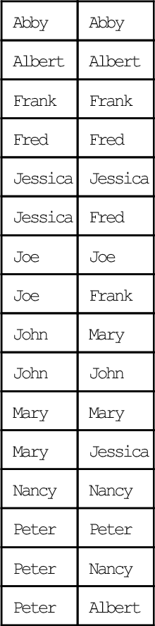
CREATE TABLE Friends
(lft_member VARCHAR(20) NOT NULL,
rgt_member VARCHAR(20) NOT NULL,
PRIMARY KEY (lft_member, rgt_member));
INSERT INTO Friends (lft_member, rgt_member)
VALUES
('John', 'Mary'),
('Mary', 'Jessica'),
('Peter', 'Albert'),
('Peter', 'Nancy'),
('Abby', 'Abby'),
('Jessica', 'Fred'),
('Joe', 'Frank'),
32.11.3 Reflexive Rows
The first thing we noticed is that only Abby has a reflexive property row. We need to add those rows and can do this with basic set operators. But it is not that easy, as you can see with this insertion statement:
INSERT INTO Friends
SELECT X.lft_member, X.rgt_member
FROM
((SELECT lft_member, lft_member FROM Friends AS F1
UNION
SELECT rgt_member, rgt_member FROM Friends AS F2)
EXCEPT
SELECT lft_member, rgt_member FROM Friends AS F3)
AS X (lft_member, rgt_member);
The use of table aliases is tricky. You have to be sure that the SQL engine will construct a table in such a way that you do not get scoping problems. The UNION and EXCEPT operators are used to assure that we do not have primary key violations.
32.11.4 Symmetric Rows
Look at the update table and there are no { (a, b), (b, a)} pairs. We need to add this second property to the relation table. This follows the pattern of set operators we just used:
INSERT INTO Friends
SELECT X.lft_member, X.rgt_member
 FROM
(
(SELECT F1.rgt_member, F1.lft_member
FROM Friends AS F1
WHERE F1.lft_member <> F1.rgt_member)
EXCEPT
(SELECT F2.lft_member, F2.rgt_member FROM Friends AS F2)
) AS X (lft_member, rgt_member);
This will give us:
| Abby | Abby |
| Albert | Peter |
| Albert | Albert |
| Frank | Joe |
| Frank | Frank |
| Fred | Jessica |
| Fred | Fred |
| Jessica | Mary |
| Jessica | Jessica |
| Jessica | Fred |
| Joe | Joe |
| Joe | Frank |
| John | Mary |
| John | John |
| Mary | Mary |
| Mary | John |
| Mary | Jessica |
| Nancy | Peter |
| Nancy | Nancy |
| Peter | Peter |
| Peter | Nancy |
| Peter | Albert |
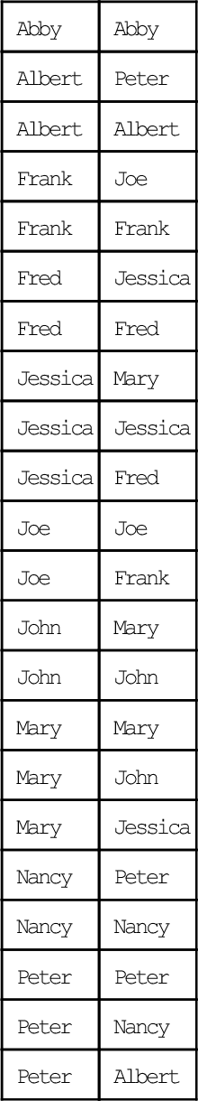
If you do quick GROUP BY query, you see that Abby is seriously antisocial with a count of 1, but Mary and Jessica look very social with a count of 3. This is not quite true because the property could be the dreaded “Rock-paper-scissors-lizard-Spock” relationship. But this is what we are using.
32.11.5 Transitive Rows
Transitivity goes on forever. Well, until we have what mathematicians call a closure. This means we have gotten the complete set of elements that can be selected by following the transitive relationship. In some cases, these sets are infinite. But in database, we can only have insanely large tables. Let’s pull a subset that is part of a clique of four friends.
Now apply the transitive relation to get some of the missing edges of a graph:
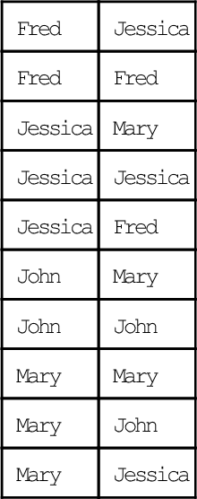
INSERT INTO Friends
SELECT X.lft_member, X.rgt_member
FROM
((SELECT F1.lft_member, F2.rgt_member
FROM Friends AS F1, Friends AS F2
WHERE F1.rgt_member = F2.lft_member)
EXCEPT
(SELECT F3.lft_member, F3.rgt_member FROM Friends AS F3)
) AS X (lft_member, rgt_member);
This is a simple statement using the definition of transitivity, without a universal quantifier or loop on it. It will add these rows to this subset:
When you look at Mary and Jessica, you have all their friends because they are directly connected. However, Fred and John do not know that they are friends. So we invoke the statement again and get those two rows. If you try it a third time, there are zero rows added.
The first thought is this sounds like a job for a recursive statement. But it is not that easy. If the original graph has a cycle in it, you can hang in an infinite loop if you try to use a recursive CTE. The assumption is that each clique has a spanning graph in the pairs in. Oops! New term: a spanning graph is a subgraph that includes the nodes and some or all of the edges of the graph. A complete graph is the spanning graph that has all the possible edges, so each node is directly connected to any other node.
32.11.6 Cliques
Now change your mindset from graphs to sets. Let’s look at the size of the cliques:
WITH X (member, clique_size)
AS
(SELECT lft_member, COUNT(*) FROM Friends GROUP BY lft_member)
SELECT * FROM X ORDER BY clique_size;
What we want to do is assign a number to each clique. This sample data is biased by the fact that the cliques are all different size. You cannot simply use the size to assign a clique_nbr.
Create this table; load it with the names.
CREATE TABLE Cliques
(clique_member VARCHAR(20) NOT NULL PRIMARY KEY,
clique_nbr INTEGER);
We can start by assigning everyone their own clique, using whatever your favorite method is
INSERT INTO Cliques
VALUES
('Abby', 1),
('Frank', 2),
('Joe', 3),
('Nancy', 4),
('Peter', 5),
('Albert', 6),
('Fred', 7),
('Jessica', 8),
('John', 9),
('Mary', 10);
Everyone is equally a member of their clique in this model. That means we could start with anyone to get the rest of their clique. The update is very straight forward. Take any clique number; find the member to whom it belongs and use that name to build that clique. But which number do we use? We could use the MIN, MAX, or a random number in the clique; I will use the MAX for no particular reason.
I keep thinking that there is a recursive update statement that will do this in one statement. But I know it will not port (Standard SQL has no recursive update statement right now. We would do it with SQL/PSM or a host language.) and I think it would be expensive. Recursion will happen for each member of the whole set, but if we consolidate a clique for one person, we have removed his friends from consideration.
The worst situation would be a bunch of hermits, so the number of clique would be the cardinality of set. That is not likely or useful in the real world. Let’s put the update in the body of a loop.
BEGIN
DECLARE in_clique_loop INTEGER;
DECLARE in_mem CHAR(10);
SET in_clique_loop = (SELECT MAX(clique_nbr) FROM Cliques);
WHILE in_clique_loop > 0
DO
SET in_mem = (SELECT clique_member FROM Cliques WHERE clique_nbr = in_clique_loop);
UPDATE Cliques
 SET clique_nbr
= (SELECT clique_nbr
FROM Cliques
 WHERE clique_member = in_mem)
WHERE clique_member
 IN (SELECT rgt_member
 FROM Friends
WHERE lft_member = in_mem);
SET in_clique_loop = in_clique_loop - 1;
END WHILE;
END;
As a programming assignment, replace the simple counting loop with one that does not do updates with clique_loop values that were removed in the prior iteration. This can save a lot of work in a larger social network than the sample data used here.
Now that we have a cliques table, we can do a simple insertion if the new guy belongs to one clique. However, we can have someone who knows a people in different cliques. This will merge the two cliques into one.
CREATE PROCEDURE Clique_Merge
(IN clique_member_1 CHAR(10),
IN clique_member_2 CHAR(10))
LANGUAGE SQL
BEGIN
UPDATE Cliques
SET clique_nbr
=(SELECT MAX(clique_nbr)
 FROM Cliques
WHERE clique_member
 IN (in_clique_member_1, in_clique_member_2))
WHERE clique_nbr
=(SELECT MIN (clique_nbr)
 FROM Cliques
WHERE clique_member
 IN (in_clique_member_1, in_clique_member_2));
END;
Deleting a member or moving him to another clique is trivial.