Keys, Locators, and Generated Values
Key is an unfortunate term in IT. We have encryption keys, sort keys, access keys, and probably a dozen other uses for the term I cannot think of right now. Unless I explicitly say otherwise, I will mean a relational key in this book. A (relational) key is a subset of one or more columns in a table which are guaranteed unique for all possible rows. If there is more than one column in the subset, this is a compound key. We have seen the UNIQUE and PRIMARY KEY constraints in Chapter 3; now let’s discuss how to use them properly.
The concept of a (relational) key is central to RDBMS, but it tactfully goes back to a fundamental law of logic known as the Law of Identity. It is the first of the three classical laws of thought. It states that: “each thing is the same as itself,” often stated as “A is A.” This means each entity is composed of its own unique set of attributes, which the ancient Greeks called its essence. Consequently, things that have the same essence are the same thing, while things that have different essences are different things.
I like the longer definition: “To be is to be something in particular; to be nothing in particular or everything in general is to be nothing at all” because it makes you focus on a clear definition. The informal logical fallacy of equivocation is using the same term with different meanings. This happens in data modeling when we have vague terms in specifications.
Thanks to Ayn Rand, Aristotle gets credit for this law, but it is not his invention (Google it). Aristotle did “invent” noncontradiction (a predicate cannot be both true and false at the same time) and the excluded middle (a predicate is either true or false).
A table is made of rows; each row models an entity or a relationship. Each entity has an identity in the logical sense (do not confuse it with the vendor’s IDENTITY feature that numbers the physical records on a particular disk drive). We use this key, this logical identity, to find a row in a table in SQL.
This is totally different from magnetic tape file systems which use a record count to locate a physical record on the tape. This pure sequential-only access made having a sort key important for tape files; doing a random access search would take far too long to be practical!
This is totally different from random access disk file systems which use pointers and indexes to locate a physical record on a particular physical disk. These systems depend on searching pointer chains in various structures such as various flavors of tree indexes, junction tables, join tables, linked lists, etc.
We do not care how the SQL engine eventually locates the data in persistent storage. We do not care if the data is moved to new locations. One SQL might use B-Tree indexes and another use hashing, but the SQL stays the same. In fact, we do not care if the data has any actual physical existence at all! A virtual table, a derived table, CTE, and VIEW are assembled by the SQL engine when the data is needed.
4.1 Key Types
The keys, logical and physical, for a table can be classified by their behavior and their source. Here is a quick table of my classification system.
| Natural Key | Artificial Key | Exposed Physical Locator | Surrogate Key | |
| Constructed from real attributes | Y | N | N | Y |
| Verifiable in reality | Y | N | N | N |
| Verifiable in itself | Y | Y | N | N |
| Visible to the user | Y | Y | Y | N |
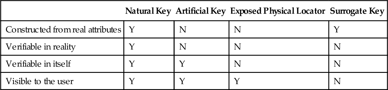
Now let’s define terms in detail.
4.1.1 Natural Keys
A natural key is a subset of attributes that occur in a table and act as a unique identifier. The user sees them. You can go to the external reality and verify them. Example: bar codes on consumer goods (read the package), geographic coordinates (get a GPS), or the VIN on an automobile (read the tag riveted to the dashboard, etched into the windows, and engraved on the engine block).
Newbies worry about a natural compound key becoming very long. Yes, short keys are nice for people. My answer is: So what? Since it is a key, you will have to add a UNIQUE constraint to have a valid schema. I will argue that this is the twenty-first century and we have much better computers than we did in the 1950s when key size was a real physical issue.
Replacing a natural two or three integer compound key with a huge GUID that no human being or other system can possibly understand because they think it will be faster only cripples the system and makes it more error-prone. I know how to verify the (longitude, latitude) pair of a location; how do you verify the GUID assigned to it?
A long key is not always a bad thing for performance. For example, if I use (city, state) as my key, I can get a free index on just (city) in many systems. I can also add extra columns to the key to make it a super-key when such a super-key gives me a covering index (i.e., an index which contains all of the columns required for a query, so that the base table does not have to be accessed at all).
4.1.2 Artificial Keys
An artificial key is an extra attribute added to the table that is seen by the user. It does not exist in the external reality but can be verified for syntax or check digits inside itself. Example: the open codes in the UPC/EAN scheme that a user can assign to his own stuff.
For example, a grocery store not only sells packaged good with preprinted bar codes but also bakes bread in the store and labels them with an open code. The check digits still work, but you have to verify them inside your own enterprise.
Experienced database designers insist on industry standard codes, such as UPC/EAN, VIN, GTIN, ISBN, etc., as keys. They know that they need to verify the data against the reality they are modeling. A trusted external source is a good thing to have. I know why this VIN is associated with this car, but why is a proprietary vendor autonumber value of 42 on one machine associated with this car? Try to verify the relationship in the reality you are modeling. It makes as much sense as locating a car by its parking space number.
4.1.3 Exposed Physical Locators
An exposed physical locator is not based on attributes in the data model but on the storage used and is exposed to user. There is no way to predict it or verify it. The system obtains a value through some physical process totally unrelated to the logical data model. The user cannot change them without destroying the relationships among the data elements.
Examples would be physical row locations encoded as a number, string, or even a proprietary data type. If hash values were accessible in an SQL product, then they would qualify, but they are usually hidden from the user.
Many programmers object to putting IDENTITY and other autonumbering devices into this category. To convert the number into a physical location requires an index search, but the concept is the same. The hardware gives you a way to go directly to a physical location which has nothing to do with the logical data model, and which cannot be changed in the physical database, or verified externally. Again, this is locating a car by its parking space number in one garage.
Most of the time, exposed physical locators are used for faking a sequential file’s positional record number, so I can reference the physical storage location—a 1960s ISAM file in SQL. You lose all the advantages of an abstract data model, SQL set oriented programming, carry extra data, and destroy the portability of code.
The early SQLs were based on preexisting file systems. The data was kept in physically contiguous disk pages, in physically contiguous rows, made up of physically contiguous columns, in short, just like a deck of punch cards or a magnetic tape. Most programmers still carry that mental model, which is why I keep ranting about file versus table, row versus record, and column versus field.
But physically contiguous storage is only one way of building a relational database and it is not the best one. The basic idea of a relational database is that user is not supposed to know how or where things are stored at all, much less write code that depends on the particular physical representation in a particular release of a particular product on particular hardware at a particular time. This is discussed in the section on IDENTITY columns.
Finally, an appeal to authority, with a quote from Dr. Codd: “… Database users may cause the system to generate or delete a surrogate, but they have no control over its value, nor is its value ever displayed to them….”
This means that a surrogate ought to act like an index: created by the user, managed by the system, and NEVER seen by a user. That means never used in code, DRI, or anything else that a user writes.
Codd also wrote the following:
There are three difficulties in employing user-controlled keys as permanent surrogates for entities.
(1) The actual values of user-controlled keys are determined by users and must therefore be subject to change by them (e.g. if two companies merge, the two employee databases might be combined with the result that some or all of the serial numbers might be changed).
(2) Two relations may have user-controlled keys defined on distinct domains (e.g. one uses social security numbers, while the other uses employee serial numbers) and yet the entities denoted are the same.
(3) It may be necessary to carry information about an entity either before it has been assigned a user-controlled key value or after it has ceased to have one (e.g. an applicant for a job and a retiree).
These difficulties have the important consequence that an equi-join on common key values may not yield the same result as a join on common entities. A solution - proposed in part [4] and more fully in [14] - is to introduce entity domains which contain system-assigned surrogates. Database users may cause the system to generate or delete a surrogate, but they have no control over its value, nor is its value ever displayed to them.....
Codd, E. Extending the Database Relational Model to Capture More Meaning, ACM Transactions on Database Systems, 4(4), pp. 397-434, 1979.
4.2 Practical Hints for Denormalization
The subject of denormalization is a great way to get into religious wars. At one extreme, you will find relational purists who think that the idea of not carrying a database design to at least 5NF is a crime against nature. At the other extreme, you will find people who simply add and move columns all over the database with ALTER statements, never keeping the schema stable.
The reason given for denormalization was performance. A fully normalized database requires a lot of JOINs to construct common VIEWs of data from its components. JOINs used to be very costly in terms of time and computer resources, so by “preconstructing” the JOIN in a denormalized table could save quite a bit of computer time. Today, we have better hardware and software. The VIEWs can be materialized and indexed if they are used frequently by the sessions. Today, only data warehouses should be denormalized and never a production OLTP system. The extra procedural code needed to maintain the data integrity of a denormalized schema is just not worth it.
Today, however, only data warehouses should be denormalized. JOINs are far cheaper than they were and the overhead of handling exceptions with procedural code is far greater than any extra database overhead.
4.2.1 Row Sorting
Back on May 27, 2001, Fred Block posted a problem on the SQL Server Newsgroup. I will change the problem slightly, but the idea was that he had a table with five character string columns that had to be sorted alphabetically within each row. This “flatten table” is a very common denormalization, which might involve months of the year as columns or other things which are acting as repeating groups in violation of First Normal Form.
Let’s declare the table to look like this and dive into the problem.
CREATE TABLE Foobar
(key_col INTEGER NOT NULL PRIMARY KEY,
c1 VARCHAR(20) NOT NULL,
c2 VARCHAR(20) NOT NULL,
c3 VARCHAR(20) NOT NULL,
c4 VARCHAR(20) NOT NULL,
c5 VARCHAR(20) NOT NULL);
This means that we want this condition to hold:
CHECK ((c1 <= c2) AND (c2 <= c3)
 AND (c3 <= c4) AND (c4 <= c5))
Obviously, if he had added this constraint to the table in the first place, we would be fine. Of course, that would have pushed the problem to the front end and I would not have a topic for this section in the book.
What was interesting was how everyone that read this Newsgroup posting immediately envisioned a stored procedure that would take the five values, sort them, and return them to their original row in the table. The only way to make this approach work for the whole table was to write an update cursor and loop through all the rows of the table. Itzik Ben-Gan posted a simple procedure that loaded the values into a temporary table, and then pulled them out in sorted order, starting with the minimum value, using a loop.
Another trick is the Bose-Nelson sort (Bose, R. C., Nelson, R. J. A Sorting Problem Journal of the ACM, 9, 282-296), that I had written about in DR. DOBB’S JOURNAL back in 1985. This is a recursive procedure that takes an integer and then generates swap pairs for a vector of that size. A swap pair is a pair of position numbers from 1 to (n) in the vector which need to be exchanged if their contents are out of order. These swap pairs are also related to Sorting Networks in the literature (see Knuth, D. The Art of Computer Programming, vol. 3, ISBN 978-0201896855).
There are other algorithms for producing Sorting Networks which produce swap pairs for various values of (n). The algorithms are not always optimal for all values of (n). You can generate them at http://jgamble.ripco.net/cgi-bin/nw.cgi?inputs=5&algorithm=best&output=svg
You are probably thinking that this method is a bit weak because the results are only good for sorting a fixed number of items. But a table only has a fixed number of columns, so that is not such a problem in SQL.
You can set up a sorting network that will sort five items (I was thinking of a Poker hand), with the minimal number of exchanges, nine swaps, like this:
Swap(c1, c2);
Swap(c4, c5);
Swap(c3, c5);
Swap(c3, c4);
Swap(c1, c4);
Swap(c1, c3);
Swap(c2, c5);
Swap(c2, c4);
Swap(c2, c3);
You might want to deal yourself a hand of five playing cards in one suit to see how it works. Put the cards face down in a line on the table and pick up the pairs, swapping them if required, then turn over the row to see that it is in sorted order when you are done.
In theory, the minimum number of swaps needed to sort (n) items is CEILING (log2 (n!)) and as (n) increases, this approaches O(nlog2(n)). The Computer Science majors will remember that “Big O” expression as the expected performance of the best sorting algorithms, such as Quicksort. The Bose-Nelson method is very good for small values of (n). If (n < 9) then it is perfect, actually. But as things get bigger, Bose-Nelson approaches O(n 1.585). In English, this method is good for a fixed size list of 16 or fewer items and goes to hell after that.
The obvious direct way to write a sorting network in SQL is as a sequence of UPDATE statements. Remember that in SQL, the SET clause assignments happen in parallel, so you can easily write a SET clause that exchanges several pairs of columns in that one statement. Using the above swap chain, we get this block of code:
BEGIN ATOMIC
-- Swap(c1, c2);
UPDATE Foobar
SET c1 = c2, c2 = c1
WHERE c1 > c2;
-- Swap(c4, c5);
UPDATE Foobar
SET c4 = c5, c5 = c4
WHERE c4 > c5;
-- Swap(c3, c5);
UPDATE Foobar
SET c3 = c5, c5 = c3
WHERE c3 > c5;
-- Swap(c3, c4);
UPDATE Foobar
SET c3 = c4, c4 = c3
WHERE c3 > c4;
-- Swap(c1, c4);
UPDATE Foobar
SET c1 = c4, c4 = c1
WHERE c1 > c4;
-- Swap(c1, c3);
UPDATE Foobar
SET c1 = c3, c3 = c1
WHERE c1 > c3;
-- Swap(c2, c5);
UPDATE Foobar
SET c2 = c5, c5 = c2
WHERE c2 > c5;
-- Swap(c2, c4);
UPDATE Foobar
SET c2 = c4, c4 = c2
WHERE c2 > c4;
-- Swap(c2, c3);
UPDATE Foobar
SET c2 = c3, c3 = c2
WHERE c2 > c3;
END;
If you look at the first two UPDATE statements, you can see that they do not overlap. This means you could roll them into one statement like this:
-- Swap(c1, c2) AND Swap(c4, c5);
UPDATE Foobar
SET c1 = CASE WHEN c1 <= c2 THEN c1 ELSE c2 END,
c2 = CASE WHEN c1 <= c2 THEN c2 ELSE c1 END,
c4 = CASE WHEN c4 <= c5 THEN c4 ELSE c5 END,
c5 = CASE WHEN c4 <= c5 THEN c5 ELSE c4 ENDWHERE c4 > c5 OR c1 > c2;
The advantage of doing this is that you have to execute only one UPDATE statement and not two. In theory, they will execute in parallel in SQL. Updating a table, even on nonkey columns, usually locks the table and prevents other users from getting to the data. If you could roll the statements into one single UPDATE, you would have the best of all possible worlds, but I doubt that the code would be easy to read.
Here are some Sorting Networks for common numbers of items, such as 12 for months in a year, 10, and 25.
n = 5: 9 comparisons in 6 parallel operations.
[[0,1],[3,4]]
[[2,4]]
[[2,3],[1,4]]
[[0,3]]
[[0,2],[1,3]]
[[1,2]]
n = 10: 29 comparisons in 9 parallel operations.
[[4,9],[3,8],[2,7],[1,6],[0,5]]
[[1,4],[6,9],[0,3],[5,8]]
[[0,2],[3,6],[7,9]]
[[0,1],[2,4],[5,7],[8,9]]
[[1,2],[4,6],[7,8],[3,5]]
[[2,5],[6,8],[1,3],[4,7]]
[[2,3],[6,7]]
[[3,4],[5,6]]
[[4,5]]
n = 12: 39 comparisons in 9 parallel operations.
[[0,1],[2,3],[4,5],[6,7],[8,9],[10,11]]
[[1,3],[5,7],[9,11],[0,2],[4,6],[8,10]]
[[1,2],[5,6],[9,10],[0,4],[7,11]]
[[1,5],[6,10],[3,7],[4,8]]
[[5,9],[2,6],[0,4],[7,11],[3,8]]
[[1,5],[6,10],[2,3],[8,9]]
[[1,4],[7,10],[3,5],[6,8]]
[[2,4],[7,9],[5,6]]
[[3,4],[7,8]]
When (n) gets larger than 16, we do not have proof that a particular sorting network is optimal. Here is a quick table of the number of comparisons for the best networks under (n = 16).
