Trees and Hierarchies in SQL
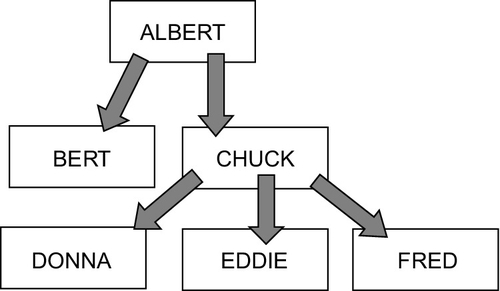
A tree is a special kind of directed graph. Graphs are data structures that are made up of nodes (usually shown as boxes) connected by edges (usually shown as lines with arrowheads). Each edge represents a one-way relationship between the two nodes it connects. In an organizational chart, the nodes are employees and each edge is the “reports to” relationship. In a parts explosion (also called a bill of materials), the nodes are assembly units (eventually resolving down to individual parts) and each edge is the “is made of” relationship.
The top of the tree is called the root. In an organizational chart, it is the highest authority; in a parts explosion, it is the final assembly. The number of edges coming out of the node is its outdegree, and the number of edges entering it is its indegree. A binary tree is one in which a parent can have at most two subordinates; more generally, an n-ary tree is one in which a node can have at most outdegree of (n).
The nodes of the tree that have no subtrees beneath them are called the leaf nodes. In a parts explosion, they are the individual parts, which cannot be broken down any further. The descendants, or subordinates, of a node (called the parent) are every node in the subtree that has the parent node as its root.
There are several ways to define a tree: It is a graph with no cycles; it is a graph where all nodes except the root have indegree 1 and the root has indegree zero. Another defining property is that a path can be found from the root to any other node in the tree by following the edges in their natural direction.
All of Western thought has been based on hierarchies and top-down organizations. It should be no surprise that hierarchies were very easy to represent in hierarchical databases, where the structure of the data and the structure of the database were the same. IMS, IDMS, Total, and other early databases used pointer chains to build graph structures that could be traversed with procedural code.
The early arguments against SQL were largely based on the lack of such traversals in a declarative language. Dr. Codd himself introduced the adjacency list mode for trees in an early paper. This model dominated SQL programming for years, even though it is not set-oriented or declarative. It simply mimics the pointer chains from the pre-RDBMS network databases.
28.1 Adjacency List Model
Since the nodes contain the data, we can add columns to represent the edges of a tree. This is usually done in one of two ways in SQL: a single table or two tables. In the single-table representation, the edge connection appears in the same table as the node. In the two-table format, one table contains the nodes of the graph and the other table contains the edges, represented as pairs of end points. The two-table representation can handle generalized directed graphs, not just trees, so we defer a discussion of this representation here. There is very little difference in the actual way you would handle things, however. The usual reason for using a separate edge table is that the nodes are very complex objects or are duplicated and need to be kept separately for normalization.
In the single-table representation of hierarchies in SQL, there has to be one column for the identifier of the node and one column of the same data type for the parent of the node. In the organizational chart, the “linking column” is usually the employee identification number of the immediate boss_emp_id of each employee.
The single table works best for organizational charts because each employee can appear only once (assuming each employee has one and only one manager), whereas a parts explosion can have many occurrences of the same part within many different assemblies. Let us define a simple Personnel table.
CREATE TABLE Personnel
(emp_id CHAR(20) NOT NULL PRIMARY KEY
CHECK (emp_id <> boss_emp_id), -- simple cycle check
boss_emp_id CHAR(20), -- he has to be NULL-able!
salary_amt DECIMAL(6,2) NOT NULL
CHECK(salary_amt > 0.00));
This is a skeleton table and should not be used. There are no constraints to prevent cycles other than the simple case that nobody can be his own boss_emp_id. There is no constraint to assure one and only one root node in the tree. Yet this is what you will find in actual code (Figure 28.1).
28.2 Finding the Root Node
The root of the tree has a boss_emp_id that is NULL—the root has no superior.
SELECT *
FROM Personnel
WHERE boss_emp_id IS NULL;
28.3 Finding Leaf Nodes
A leaf node is one that has no subordinates under it. In an adjacency list model, this set of nodes is fairly easy to find. They are going to be the employees who are not bosses to anyone else in the company, thus:
SELECT *
FROM Personnel AS P1
WHERE NOT EXISTS (SELECT *
 FROM Personnel AS P2
WHERE P1.emp_id = P2.boss_emp_id);
28.4 Finding Levels in a Tree
The length of a path from one node to another is measured by the number of levels of the hierarchy that you have to travel to get from the start to the finish. This is handy for queries such as “Does Mr. King have any authority over Mr. Jones?” or “Does a gizmo use a frammistat?” which are based on paths. To find the name of the boss_emp_id for each employee, the query is a self-JOIN, like this:
SELECT B1.boss_emp_id, P1.emp_id
FROM Personnel AS B1, Personnel AS P1
WHERE B1.boss_emp_id = P1.boss_emp_id;
But something is missing here. These are only the immediate bosses of the employees. Your boss_emp_id’s boss_emp_id also has authority over you, and so forth up the tree until we find someone who has no subordinates. To go two levels deep in the tree, we need to do a more complex self-JOIN, thus:
SELECT B1.boss_emp_id, P2.emp_id
FROM Personnel AS B1, Personnel AS P1, Personnel AS P2
WHERE B1.boss_emp_id = P1.boss_emp_id
AND P1.emp_id = P2.boss_emp_id;
To go more than two levels deep in the tree, just extend the pattern. Unfortunately, you have no idea just how deep the tree is, so you must keep extending this query until you get an empty set back as a result. Another method is to declare a CURSOR and traverse the tree with procedurally. This is usually very slow, but it will work for any depth of tree. The third way is to use a recursive CTE. We will discuss CTEs later, but for now look at this example.
WITH RECURSIVE Subordinates (root_emp_id, emp_id, level)
AS
(SELECT P1.boss_emp_id, P1.emp_id, 0
FROM Personnel AS P1
UNION ALL
SELECT S.root_emp_id, P2.emp_id, (S.level + 1)
FROM Personnel AS P2, Subordinates AS S
WHERE P2.boss_emp_id = S.emp_id)
SELECT * FROM Subordinates;
The anchor or fixpoint of the recursion is in the first SELECT. The second SELECT references the CTE, Subordinates, as a whole and joins to its rows. This UNION ALL is done over and over until it returns an empty set. The basic pattern we used to compute the organizational level can be used for hierarchical aggregations.
None of these queries are cheap to execute, but the recursive CTE is portable and go or any depth of hierarchy. It is usually a cursor and loop under the covers, it is a bitch to optimize even in theory.
28.5 Tree Operations
Tree operations are those that alter the size and shape of a tree, not the contents of the nodes of the tree. Some of these operations can be very complex, such as balancing a binary tree, but we will deal only with deletion and insertion of a whole subtree.
28.5.1 Subtree Deletion
Deleting a subtree is hard in the adjacency list model. You have to find all of the subordinates and then remove that subset from the table. One way of doing this is with a cursor, but you can also mark the subordinates and then delete them:
BEGIN ATOMIC
UPDATE Personnel
SET boss_emp_id = '???????' -- deletion marker
WHERE boss_emp_id = :subtree_root;
LOOP UPDATE Personnel -- mark subordinates
SET emp_id = CASE WHEN boss_emp_id = '???????'
THEN '???????' ELSE emp_id END,
boss_emp_id = CASE WHEN EXISTS
(SELECT *
FROM Personnel AS P1
WHERE P1.emp_id = Personnel.boss_emp_id
AND Personnel.boss_emp_id = '???????')
THEN '???????' ELSE boss_emp_id END;
END LOOP;
DELETE FROM Personnel  -- delete marked nodes
WHERE boss_emp_id = '???????';
END;
Obviously, you do not want to use a marker which has any real meaning in the table.
28.5.2 Subtree Insertion
Inserting a subtree under a given node is easy. Given a table with the subtree that is to be made subordinate to a given node, you simply write:
BEGIN
-- subordinate the subtree to his new boss_emp_id
INSERT INTO Personnel VALUES (:subtree_root, :new_boss_emp_id, …);
-- insert the subtree
INSERT INTO Personnel SELECT * FROM Subtree;
END;
Remember that a single row is just a subtree with one node, so you will that people will not try to build a subtree table. They mimic what they did with punch cards and sequential files; single row insertion statements.
28.6 Nested Sets Model
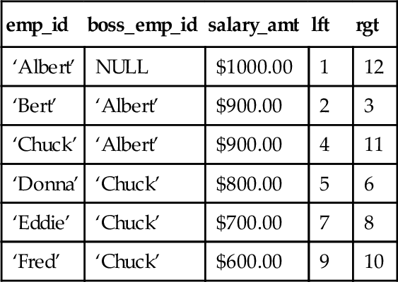
Since SQL is a set-oriented language, nested sets is a better model for trees and hierarchies. Let us redefine our simple Personnel table. The first three columns explain themselves and recopy from Section28.1. Ignore the lft and rgt columns for now, but note that their names are abbreviations for “left” and “right,” which are reserved words in ANSI/ISO Standard SQL (Figure 28.2).
CREATE TABLE Personnel
(emp_id CHAR(10) NOT NULL PRIMARY KEY,
boss_emp_id CHAR(10), -- this has to be NULL-able for the root node!!
salary_amt DECIMAL(6,2) NOT NULL,
lft INTEGER NOT NULL,
rgt INTEGER NOT NULL);
Personnel
| emp_id | boss_emp_id | salary_amt | lft | rgt |
| ‘Albert’ | NULL | $1000.00 | 1 | 12 |
| ‘Bert’ | ‘Albert’ | $900.00 | 2 | 3 |
| ‘Chuck’ | ‘Albert’ | $900.00 | 4 | 11 |
| ‘Donna’ | ‘Chuck’ | $800.00 | 5 | 6 |
| ‘Eddie’ | ‘Chuck’ | $700.00 | 7 | 8 |
| ‘Fred’ | ‘Chuck’ | $600.00 | 9 | 10 |
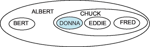
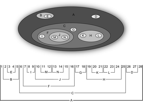
Which would look like this as a graph (Figure 28.2): To show a tree as nested sets, replace the boxes with ovals and then nest subordinate ovals inside their parents. Containment represents subordination. The root will be the largest oval and will contain every other node. The leaf nodes will be the innermost ovals, with nothing else inside them, and the nesting will show the hierarchical relationship. This is a natural way to model a parts explosion, as a final assembly is made of physically nested assemblies that finally break down into separate parts. This tree translates into this nesting of sets (Figures 28.2 and 28.3). Using this approach, we can model a tree with lft and rgt nested sets with number pairs. These number pairs will always contain the pairs of their subordinates so that a child node is within the bounds of its parent. This is a version of the nested sets, flattened onto a number line (Figure 28.4). If that mental model does not work for you, then visualize the nested sets model as a little worm with a Bates automatic numbering stamp crawling along the “boxes-and-arrows” version of the tree. The worm starts at the top, the root, and makes a complete trip around the tree. When he comes to a node, he puts a number in the cell on the side that he is visiting and his numbering stamp increments itself. Each node will get two numbers, one for the right (rgt) side and one for the left (lft) side. Computer science majors will recognize this as a modified preorder tree traversal algorithm. This numbering has some predictable results that we can use for building queries.
28.7 Finding Root and Leaf Nodes
The root will always have a 1 in its lft column and twice the number of nodes in its rgt column. This is easy to understand; the worm has to visit each node twice, once for the lft side and once for the rgt side, so the final count has to be twice the number of nodes in the whole tree. The root of the tree is found with the query.
SELECT *
 FROM Personnel
 WHERE lft = 1;
This query will take advantage of the index on the lft value. In the nested sets table, the difference between the lft and rgt values of leaf nodes is always 1. Think of the little worm turning the corner as he crawls along the tree. That means you can find all leaf nodes with the extremely simple query.
SELECT *
 FROM Personnel
 WHERE lft = (rgt- 1);
There is a further trick, to speed up queries. Build a unique index on either the lft column or on the pair of columns (lft, rgt) and then you can rewrite the query to take advantage of the index.
Did you notice that ((rgt − lft + 1) is the size of the subtree at this node? This is the algebraic property of nested sets. It depends on incrementing the lft and rgt values to work.
28.8 Finding Subtrees
Another very useful mathematical property is that any node in the tree is the root of a subtree (the leaf nodes are a degenerate case). In the nested sets table, all the descendants of a node can be found by looking for the nodes with a rgt and lft number between the lft and rgt values of their parent node. This is the containment property.
For example, to find out all the subordinates of each boss_emp_id in the corporate hierarchy, you would write:
SELECT Mangers.emp_id AS boss, Workers.emp_id AS worker
FROM Personnel AS Mgrs, Personnel AS Workers
WHERE Workers.lft BETWEEN Mgrs.lft AND Mgrs.rgt
AND Workers.rgt BETWEEN Mgrs.lft AND Mgrs.rgt;
Look at the way the numbering was done, and you can convince yourself that this search condition is too strict. We can drop the last predicate and simply use:
SELECT Mangers.emp_id AS boss, Workers.emp_id AS worker
FROM Personnel AS Mgrs, Personnel AS Workers
WHERE Workers.lft BETWEEN Mgrs.lft AND Mgrs.rgt;
This would tell you that everyone is also his own superior, so in some situations, you would also add the predicate.
.. AND Workers.lft <> Mgrs.lft
This simple self-JOIN query is the basis for almost everything that follows in the nested sets model.
28.9 Finding Levels and Paths in a Tree
The level of a node in a tree is the number of edges between the node and the root, where the larger the depth number, the farther away the node is from the root. A path is a set of edges which directly connect two nodes.
The nested sets model uses the fact that each containing set is “wider” (where width = (rgt − lft)) than the sets it contains.
Obviously, the root will always be the widest row in the table. The level function is the number of edges between two given nodes; it is fairly easy to calculate. For example, to find the level of each worker, you would use:
SELECT P2.emp_id, (COUNT(P1.emp_id) - 1) AS level
FROM Personnel AS P1, Personnel AS P2
WHERE P2.lft BETWEEN P1.lft AND P1.rgt
GROUP BY P2.emp_id;
The reason for using the expression (COUNT(*) − 1) is to remove the duplicate count of the node itself because a tree starts at level zero. If you prefer to start at one, then drop the extra arithmetic.
28.9.1 Finding the Height of a Tree
The height of a tree is the length of the longest path in the tree. We know that this path runs from the root to a leaf node, so we can write a query to find like this:
SELECT MAX(level) AS height
FROM (SELECT P2.emp_id, (COUNT(P1.emp_id) - 1)
 FROM Personnel AS P1, Personnel AS P2
 WHERE P2.lft BETWEEN P1.lft AND P1.rgt
 GROUP BY P2.emp_id) AS L(emp_id, level);
Other queries can be built from this tabular subquery expression of the nodes and their level numbers.
28.9.2 Finding Immediate Subordinates
The adjacency model allows you to find the immediate subordinates of a node immediately; you simply look in the column which gives the parent of every node in the tree.
This becomes complicated in the nested set model. You have to prune the subtree rooted at the node of boss_emp_id we are looking at to one level. Another way is to find his subordinates is to define them as personnel who have no other employee between themselves and the boss_emp_id in question.
CREATE VIEW Immediate_Subordinates (boss_emp_id, worker, lft, rgt)
AS SELECT Mgrs.emp_id, Workers.emp_id, Workers.lft, Workers.rgt
 FROM Personnel AS Mgrs, Personnel AS Workers
WHERE Workers.lft BETWEEN Mgrs.lft AND Mgrs.rgt
 AND NOT EXISTS -- no middle manger between the boss_emp_id and us!
 (SELECT *
 FROM Personnel AS MidMgr
WHERE MidMgr.lft BETWEEN Mgrs.lft AND Mgrs.rgt
 AND Workers.lft BETWEEN MidMgr.lft AND MidMgr.rgt
 AND MidMgr.emp_id NOT IN (Workers.emp_id, Mgrs.emp_id));
There is a reason for setting this up as a VIEW and including the lft and rgt numbers of the subordinates. The lft and rgt numbers for the parent can be reconstructed by
SELECT boss_emp_id, MIN(lft) - 1, MAX(rgt) + 1
  FROM Immediate_Subordinates AS S1
 GROUP BY boss_emp_id;
This illustrates a general principle of the nested sets model; it is easier to work with subtrees than to work with individual nodes or other subsets of the tree.
28.9.3 Finding Oldest and Youngest Subordinates
The third property of a nested sets model is sibling ordering. Do you remember the old Charlie Chan movies? Charlie Chan was the Chinese detective created by Earl Derr Biggers. There were 44 “Charlie Chan” movies made from 1931 to 1949. Detective Chan had varying number of children who were always helping him with his cases. The kids were referred to by their birth order, number one son, number two son, and so forth.
Organizations with a seniority system are much like the Chan family. Within each organizational level, the immediate subordinates have a left to right order implied by their lft value. The adjacency list model does not have a concept of such rankings, so the following queries are not possible without extra columns to hold the ordering in the adjacency list model. This lets you assign some significance to being the leftmost child of a parent. For example, the employee in this position might be the next in line for promotion in a corporate hierarchy.
Most senior subordinate is found by this query:
SELECT Workers.emp_id, ' is the oldest child of ', :my_employee
FROM Personnel AS Mgrs, Personnel AS Workers
WHERE Mgrs.emp_id = :my_employee
AND Workers.lft + 1 = Mgrs.lft; -- leftmost child
Most junior subordinate:
SELECT Workers.emp_id, ' is the youngest child of ', :my_employee
FROM Personnel AS Mgrs, Personnel AS Workers
WHERE Mgrs.emp_id = :my_employee
AND Workers.rgt = Mgrs.rgt - 1; -- rightmost child
The real trick is to find the nth sibling of a parent in a tree.
SELECT S1.worker, ' is the number ', :n, ' son of ', S1.boss_emp_id
FROM Immediate_Subordinates AS S1
WHERE S1.boss_emp_id = :my_employee
AND 1 = (SELECT COUNT(S2.lft) - 1
 FROM Immediate_Subordinates AS S2
 WHERE S2.boss_emp_id = S1.boss_emp_id
AND S2.boss_emp_id <> S1.worker
AND S2.lft BETWEEN 1 AND S1.lft);
Notice that you have to subtract one to avoid counting the parent as his own child. Here is another way to do this and get a complete ordered listing of siblings.
SELECT P1.emp_id AS boss_emp_id, S1.worker,
COUNT(S2.lft) AS sibling_order
FROM Immediate_subordinates AS S1,
 Immediate_subordinates AS S2,
 Personnel AS P1
WHERE S1.boss_emp_id = P1.emp_id
 AND S2.boss_emp_id = S1.boss_emp_id
 AND S2.lft <= S1.lft
GROUP BY p1.emp_id, S1.worker;
28.9.4 Finding a Path
To find and number the nodes in the path from a :start_node to a :finish_node, you can repeat the nested sets “BETWEEN predicate trick” twice to form an upper and a lower boundary on the set.
SELECT T2.node,
(SELECT COUNT(*)
FROM Tree AS T4
 WHERE T4.lft BETWEEN T1.lft AND T1.rgt
AND T2.lft BETWEEN T4.lft AND T4.rgt) AS path_nbr
FROM Tree AS T1, Tree AS T2, Tree AS T3
WHERE T1.node = :start_node
 AND T3.node = :finish_node
 AND T2.lft BETWEEN T1.lft AND T1.rgt
 AND T3.lft BETWEEN T2.lft AND T2.rgt;
Using the Parts explosion tree, this query would return the following table for the path from ‘C’ to ‘N,’ with 1 being the highest starting node and the other nodes numbered in the order they must be traversed.
However, if you just need a column to use in a sort for outputting the answer in a host language, then replace the subquery expression with “(T2.rgt − T2.lft) AS sort_col” and use an ORDER BY clause in a cursor.
28.10 Functions in the Nested Sets Model
JOINs and ORDER BY clauses will not interfere with the nested sets model as they will with the adjacency graph model. Nor are the results dependent on the order in which the rows are displayed as in vendor extensions. The LEVEL function for a given employee node is a matter of counting how many lft and rgt groupings (superiors) this employee node’s lft or rgt is within. You can get this by modifying the sense of the BETWEEN predicate in the query for subtrees:
SELECT COUNT(Mgrs.emp_id) AS level
FROM Personnel AS Mgrs, Personnel AS Workers
WHERE Workers.lft BETWEEN Mgrs.lft AND Mgrs.rgt
 AND Workers.emp_id = :my_employee;
A simple total of the salaries of the subordinates of a supervising employee works out the same way. Notice that this total will include the boss_emp_id’s salary_amt, too.
SELECT SUM (Workers.salary_amt) AS payroll
FROM Personnel AS Mgrs, Personnel AS Workers
WHERE Workers.lft BETWEEN Mgrs.lft AND Mgrs.rgt
AND Mgrs.emp_id = :my_employee;
A slightly trickier function involves using quantity columns in the nodes to compute an accumulated total. This usually occurs in parts explosions, where one assembly may contain several occurrences of a subassembly.
SELECT SUM (Subassem.qty * Subassem.price) AS totalcost
FROM Blueprint AS Assembly, Blueprint AS Subassem
WHERE Subassem.lft
 BETWEEN Assembly.lft AND Assembly.rgt
 AND Assembly.part_nbr = :this_part;
28.11 Deleting Nodes and Subtrees
Deleting a single node in the middle of the tree is conceptually harder than removing whole subtrees. When you remove a node in the middle of the tree, you have to decide how to fill the hole. There are two ways. The first method is to promote one of the subordinates to the original node’s position—Dad dies and the oldest son takes over the business. The second method is to connect the subordinates to the parent of the original node—Mom dies and the kids are adopted by Grandma.
28.11.1 Deleting Subtrees
This query will take the downsized employee as a parameter and remove the subtree rooted under him. The trick in this query is that we are using the key, but we need to get the lft and rgt values to do the work. The answer is scalar subqueries:
DELETE FROM Personnel
WHERE lft BETWEEN
(SELECT lft FROM Personnel WHERE emp_id = :downsized)
AND
(SELECT rgt FROM Personnel WHERE emp_id = :downsized);
The problem is that this will result gaps in the sequence of nested sets numbers. You can still do queries that depend on containment and sibling ordering, but the algebraic property gone. Closing the gaps is like garbage collection in other languages.
28.11.2 Deleting a Single Node
Deleting a single node in the middle of the tree is harder than removing whole subtrees. When you remove a node in the middle of the tree, you have to decide how to fill the hole. There are two ways. The first method is to connect the subordinates to the parent of the original node—Mom dies and the kids are adopted by Grandma.
Grandma gets the kids automatically in the nested sets model; you just delete the node and its subordinates are already contained in their ancestor nodes.
The second method is to promote one of the subordinates to the original node’s position—Dad dies and a chid inherits the business, usually, the oldest son. There is a problem with this operation, however. If the older child has subordinates of his own, then you have to decide how to handle them and so on down the tree until you get to a leaf node.
Let’s use a ‘??’ as a marker for the downsized employee. This way we can promote the oldest subordinate to the vacant job and then decide if we want to fill his previous position with his oldest subordinate.
BEGIN
UPDATE Personnel -- set removed emp_id to vacant position marker
SET emp_id = '??'
WHERE emp_id = :downsized;
UPDATE Personnel -- promotion
SET emp_id
= CASE Personnel.emp_id
WHEN '??' -- move oldest child into vacant position marker
THEN (SELECT P1.emp_id
FROM Personnel AS p1
 WHERE P1.lft = Personnel.lft + 1)
WHEN (SELECT P2.emp_id -- move vacant position marker into oldest child
FROM Personnel AS P1, Personnel AS P2
 WHERE (P1.lft + 1) = P2.lft
AND P1.emp_id = '??')
THEN '??'
ELSE emp_id END
WHERE NOT (emp_id = '??' AND (lft + 1 = rgt)); -- vacancy is not at leaf node
END;
28.11.3 Closing Gaps in the Tree
The important thing is to preserve the nested subsets based on lft and rgt numbers. As you remove nodes from a tree, you create gaps in the nested sets numbers. These gaps do not destroy the subset property or sibling ordering, but they can present other problems and should be closed. This is like garbage collection in other languages. The easiest way to understand the code is to break it up into a series of meaningful VIEWs and then use the VIEWs to UPDATE the tree table. This VIEW “flattens out” the whole tree into a list of nested sets numbers, regardless of whether they are lft or rgt numbers:
CREATE VIEW LftRgt(old_lftrgt, new_lftrgt)
AS
(WITH LftRgt (lftrgt)
AS
(SELECT lft from Personnel
 UNION ALL
SELECT rgt from Personnel)
SELECT lftrgt, ROW_NUMBER() OVER (ORDER BY lftrgt)
LftRgt;
UPDATE Personnel
SET lft = CASE WHEN old_lftrgt = lft
 THEN new_lftrgt
 ELSE lft END,
rgt = CASE WHEN old_lftrgt = rgt
 THEN new_lftrgt
 ELSE rgt END;
28.12 Summary Functions on Trees
There are tree queries that deal strictly with the nodes themselves and have nothing to do with the tree structure at all. For example, what is the name of the president of the company? How many people are in the company? Are there two people with the same name working here? These queries are handled with the usual SQL queries and there are no surprises.
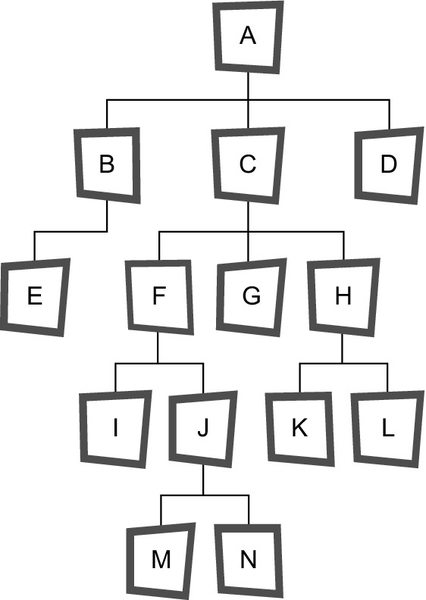
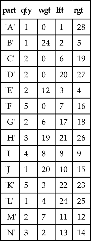
Other types of queries do depend on the tree structure. For example, what is the total weight of a finished assembly (i.e., the total of all of its subassembly weights)? Do Harry and John report to the same boss_emp_id? And so forth. Let’s consider a sample database that shows a parts explosion for a Frammis again, but this time in nested sets representation. The leaf nodes are the basic parts, the root node is the final assembly, and the nodes in between are subassemblies. Each part or assembly has a unique catalog number (in this case, a single letter), a weight, and the quantity of this unit that is required to make the next unit above it. The declaration looks like this:
CREATE TABLE Frammis
(part CHAR(2) PRIMARY KEY,
qty INTEGER NOT NULL
 CONSTRAINT non_negative_qty
 CHECK (qty >= 0),
wgt INTEGER NOT NULL
 CONSTRAINT non_negative_wgt
 CHECK (wgt >= 0),
lft INTEGER NOT NULL UNIQUE
 CONSTRAINT valid_lft
 CHECK (lft > 0),
rgt INTEGER NOT NULL UNIQUE
 CONSTRAINT valid_rgt
 CHECK (rgt > 1),
CONSTRAINT valid_range_pair
CHECK (lft < rgt));
We initially load it with this data:
Frammis
| part | qty | wgt | lft | rgt |
| ‘A’ | 1 | 0 | 1 | 28 |
| ‘B’ | 1 | 0 | 2 | 5 |
| ‘C’ | 2 | 0 | 6 | 19 |
| ‘D’ | 2 | 0 | 20 | 27 |
| ‘E’ | 2 | 12 | 3 | 4 |
| ‘F’ | 5 | 0 | 7 | 16 |
| ‘G’ | 2 | 6 | 17 | 18 |
| ‘H’ | 3 | 0 | 21 | 26 |
| ‘I’ | 4 | 8 | 8 | 9 |
| ‘J’ | 1 | 0 | 10 | 15 |
| ‘K’ | 5 | 3 | 22 | 23 |
| ‘L’ | 1 | 4 | 24 | 25 |
| ‘M’ | 2 | 7 | 11 | 12 |
| ‘N’ | 3 | 2 | 13 | 14 |
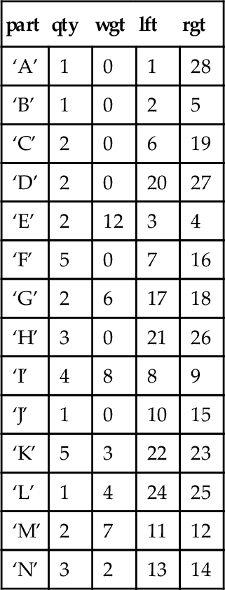
Notice that the weights of the subassemblies are initially set to zero and only parts (leaf nodes) have weights. You can easily insure this is true with this statement.
UPDATE Frammis
SET wgt = 0
WHERE lft < (rgt - 1);
The weight of an assembly will be calculated as the total weight of all its subassemblies. The tree initially looks like this (Figures 28.5–28.7).
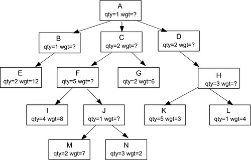


Look at the M and N leaf nodes. The table says that we need two M units weighing 7 kilograms each, plus three N units weighing 2 kilograms each, to make one J assembly. So that is ((2 * 7) + (3 * 2)) = 20 kilograms per J assembly. That is, the weight of a nonleaf node is the sum of the products of the weights and quantities of its immediate subordinates.
The problem is that the nested sets model is good at finding subtrees, but not at finding a single level within the tree. The immediate subordinates of a node are found with this view:
CREATE VIEW Immediate_Kids (parent, child, wgt)
AS
SELECT F2.part, F1.part, F1.wgt
FROM Frammis AS F1, Frammis AS F2
WHERE F1.lft BETWEEN F2.lft AND F2.rgt
AND F1.part <> F2.part
AND NOT EXISTS
(SELECT *
 FROM Frammis AS F3
 WHERE F3.lft BETWEEN F2.lft AND F2.rgt
AND F1.lft BETWEEN F3.lft AND F3.rgt
AND F3.part NOT IN (F1.part, F2.part));
The query says that F2 is the parent, and F1 is one of it’s child. The EXISTS() checks to see that there are no other descendants strictly between F1 and F2. This VIEW can then be used with this UPDATE statement to calculate the weights of each level of the Frammis.
BEGIN ATOMIC
UPDATE Frammis -- set non-leaf nodes to zero
SET wgt = 0
WHERE lft < rgt - 1;
WHILE (SELECT wgt FROM Frammis WHERE lft = 1) = 0
DO UPDATE Frammis
SET wgt
= (SELECT SUM(F1.qty * F1.wgt)
FROM Frammis AS F1
WHERE EXISTS
 (SELECT *
FROM Immediate_kids AS I1
WHERE parent = Frammis.part
AND I1.child = F1.part))
 WHERE wgt = 0 -- weight is missing
AND NOT EXISTS -- subtree rooted here is completed
(SELECT *
FROM Immediate_kids AS I2
 WHERE I2.parent = Frammis.part
AND I2.wgt = 0);
END WHILE;
END;
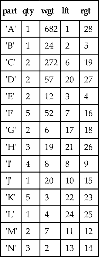
This is a bit tricky, but in English we are calculating the weights of the sub-assemblies by moving up the tree until we get to the root. A node is filled in with a weight when all of its subordinate assemblies have a weight assigned to them. The EXISTS() predicate in the WHERE clause says that this part in Frammis is a parent and the NOT EXISTS() predicate says that no sibling has a zero (i.e., unknown) weight. This query works from the leaf nodes up to the root and has been applied repeatedly.
If we change the weight of any part, we must correct the whole tree. Simply set the weight of all nonleaf nodes to zero first and redo this procedure. Once the proper weights and quantities are in place, it is fairly easy to find averages and other aggregate functions within a subtree.
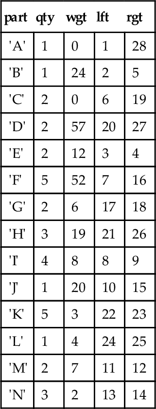
Here is how the table changes after each execution:
First iteration (7 rows affected)
| part | qty | wgt | lft | rgt |
| 'A' | 1 | 0 | 1 | 28 |
| 'B' | 1 | 24 | 2 | 5 |
| 'C' | 2 | 0 | 6 | 19 |
| 'D' | 2 | 0 | 20 | 27 |
| 'E' | 2 | 12 | 3 | 4 |
| 'F' | 5 | 0 | 7 | 16 |
| 'G' | 2 | 6 | 17 | 18 |
| 'H' | 3 | 19 | 21 | 26 |
| 'I' | 4 | 8 | 8 | 9 |
| 'J' | 1 | 20 | 10 | 15 |
| 'K' | 5 | 3 | 22 | 23 |
| 'L' | 1 | 4 | 24 | 25 |
| 'M' | 2 | 7 | 11 | 12 |
| 'N' | 3 | 2 | 13 | 14 |
Second iteration (4 rows affected)
| part | qty | wgt | lft | rgt |
| 'A' | 1 | 0 | 1 | 28 |
| 'B' | 1 | 24 | 2 | 5 |
| 'C' | 2 | 0 | 6 | 19 |
| 'D' | 2 | 57 | 20 | 27 |
| 'E' | 2 | 12 | 3 | 4 |
| 'F' | 5 | 52 | 7 | 16 |
| 'G' | 2 | 6 | 17 | 18 |
| 'H' | 3 | 19 | 21 | 26 |
| 'I' | 4 | 8 | 8 | 9 |
| 'J' | 1 | 20 | 10 | 15 |
| 'K' | 5 | 3 | 22 | 23 |
| 'L' | 1 | 4 | 24 | 25 |
| 'M' | 2 | 7 | 11 | 12 |
| 'N' | 3 | 2 | 13 | 14 |
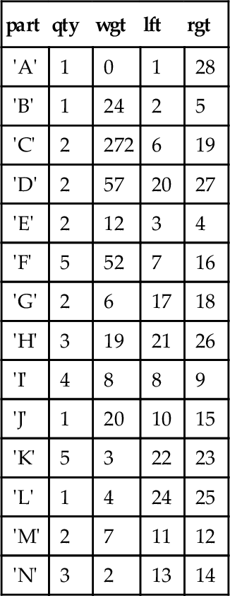
28.13 Inserting and Updating Trees
Updates to the nodes are done by searching for the key of each node; there is nothing special about them. Inserting a subtree or a new node involves finding a place in the tree for the new node, spreading the other nodes apart by incrementing their (lft, rgt) numbers, and then renumbering the new subtree to fit. For example, let’s insert a new node, G1, under part G. We can insert one node at a time like this:
BEGIN ATOMIC
DECLARE right_most_sibling INTEGER;
SET right_most_sibling
= (SELECT rgt
 FROM Frammis
WHERE part = 'G'),
UPDATE Frammis
SET lft = CASE WHEN lft > right_most_sibling
 THEN lft + 2
 ELSE lft END,
rgt = CASE WHEN rgt >= right_most_sibling
 THEN rgt + 2
 ELSE rgt END
WHERE rgt >= right_most_sibling;
INSERT INTO Frammis (part, qty, wgt, lft, rgt)
VALUES ('G1', 3, 4, parent, (parent + 1));
COMMIT WORK;
END;
The idea is to spread the lft and rgt numbers after the youngest child of the parent, G in this case, over by two to make room for the new addition, G1. This procedure will add the new node to the rightmost child position, which helps to preserve the idea of an age order among the siblings.
28.13.1 Moving a Subtree Within a Tree
Yes, it is possible to move subtrees inside the nested sets model for hierarchies. But we need to get some preliminary things out of the way first. The nested sets model needs a few auxiliary tables to help it. The first is:
CREATE VIEW LftRgt (i)
AS SELECT lft FROM Tree
UNION ALL
SELECT rgt FROM Tree;
This is all lft and rgt values in a single column. Since we should have no duplicates, we use a UNION ALL to construct the VIEW. Yes, LftRgt can be written as a derived table inside queries, but there are advantages to use a VIEW. Self-joins are much easier to construct. Code is easier to read. If more than one user needs this table, it can be materialized only once by the SQL engine.
The next table is a working table to hold subtrees that we extract from the original tree. This could be declared as a local temporary table, but it would lose the benefit of a PRIMARY KEY declaration.
CREATE TABLE WorkingTree
(root CHAR(2) NOT NULL,
node CHAR(2) NOT NULL,
lft INTEGER NOT NULL,
rgt INTEGER NOT NULL,
PRIMARY KEY (root, node));
The root column is going to be the value of the root node of the extracted subtree. This gives us a fast way to find an entire subtree via part of the primary key. While this is not important for the stored procedure discussed here, it is useful for other operations that involve multiple extracted subtrees.
Let me move right to the commented code. The input parameters are the root node of the subtree being moved and the node which is to become its new parent. In this procedure, there is an assumption that new sibling are added on the right side of the immediate subordinates so that siblings are ordered by their age.
CREATE PROCEDURE MoveSubtree
 (IN my_root CHAR(2),
 IN new_parent CHAR(2))
AS
BEGIN
DECLARE right_most_sibling INTEGER,
subtree_size INTEGER;
-- clean out and rebuild working tree
DELETE FROM WorkingTree;
INSERT INTO WorkingTree (root, node, lft, rgt)
SELECT my_root,
T1.node,
T1.lft - (SELECT MIN(lft)
FROM Tree
 WHERE node = my_root),
T1.rgt - (SELECT MIN(lft)
FROM Tree
 WHERE node = my_root)
FROM Tree AS T1, Tree AS T2
WHERE T1.lft BETWEEN T2.lft AND T2.rgt
AND T2.node = my_root;
-- Cannot move a subtree to itself, infinite recursion
IF (new_parent IN (SELECT node FROM WorkingTree))
THEN BEGIN
 PRINT 'Cannot move a subtree to itself, infinite recursion';
 DELETE FROM WorkingTree;
 END
ELSE BEGIN
 -- remove the subtree from original tree
 DELETE FROM Tree
 WHERE node IN (SELECT node FROM WorkingTree);
 -- get size and location for inserting working tree into new slot
 SET right_most_sibling
 = (SELECT rgt
 FROM Tree
 WHERE node = new_parent);
 SET subtree_size = (SELECT (MAX(rgt)+1) FROM WorkingTree);
 -- make a gap in the tree
 UPDATE Tree
SET lft = CASE WHEN lft > right_most_sibling
THEN lft + subtree_size
ELSE lft END,
rgt = CASE WHEN rgt >= right_most_sibling
THEN rgt + subtree_size
ELSE rgt END
 WHERE rgt >= right_most_sibling;
 -- insert the subtree and renumber its rows
 INSERT INTO Tree (node, lft, rgt)
 SELECT node,
lft + right_most_sibling,
rgt + right_most_sibling
FROM WorkingTree;
 -- clean out working tree table
 DELETE FROM WorkingTree;
 -- close gaps in tree
 UPDATE Tree
SET lft = (SELECT COUNT(*)
 FROM LftRgt
WHERE LftRgt.i <= Tree.lft),
rgt = (SELECT COUNT(*)
 FROM LftRgt
WHERE LftRgt.i <= Tree.rgt);
 END;
END; -- of MoveSubtree
As a minor note, the variables right_most_sibling and @subtree_size could have been replaced with their scalar subqueries in the UPDATE and INSERT INTO statements that follow their assignments. But that would make the code much harder to read at the cost of only a slight boost in performance.
28.14 Converting Adjacency List to Nested Sets Model
Most SQL databases have used the adjacency list model for two reasons. The first reason is that Dr. Codd came up with it in the early days of the relational model and nobody thought about it after that. The second reason is that the adjacency list is a way of “faking” pointer chains, the traditional programming method in procedural languages for handling trees.
It would be fairly easy to load an adjacency list model table into a host language program and then use a recursive preorder tree traversal program from a college freshman data structures textbook to build the nested sets model. This is not the fastest way to do a conversion, but since conversions are probably not going to be frequent tasks, it might be good enough when translated into your SQL product’s procedural language.
28.15 Converting Nested Sets to Adjacency List Model
To convert a nested sets model into an adjacency list model, use this query:
SELECT P.node AS parent, P.node
FROM Tree AS P
LEFT OUTER JOIN
Tree AS C
ON P.lft = (SELECT MAX(lft)
 FROM Tree AS S
WHERE P.lft > S.lft
 AND P.lft < S.rgt);
This single statement, originally written by Alejandro Izaguirre, replaces my own previous attempt that was based on a push-down stack algorithm. Once more, we see that best way to program SQL is to think in terms of sets and not procedures.
28.16 Comparing Nodes and Structure
There are several kinds of equality comparisons when you are dealing with a hierarchy:
(2) Same structure in both tables
(3) Same nodes and structure in both tables—they are identical
Let me once more invoke my semi-quasi-famous Organization chart I used earlier to show the nested sets model and a second Personnel table to which we will compare it.
Case one: Same employees
Let’s create a second table with the same nodes, but with a different structure
CREATE TABLE Personnel_2
(emp_id CHAR(10) NOT NULL PRIMARY KEY,
lft INTEGER NOT NULL UNIQUE CHECK (lft > 0),
rgt INTEGER NOT NULL UNIQUE CHECK (rgt > 1),
CONSTRAINT order_okay CHECK (lft < rgt));
Insert sample data and flatten the organization to report directly to Albert.
SELECT CASE WHEN COUNT(*) = 0
 THEN 'They have the same nodes'
 ELSE 'They are different node sets' END AS answer
FROM (SELECT emp_id, COUNT(emp_id) OVER() AS emp_cnt FROM Personnel AS P1
 EXCEPT
 SELECT emp_id, COUNT(emp_id) OVER() AS emp_cnt FROM Personnel_2 AS P2)
 AS X;
The trick in this query is including the row count in a windowed function.
Case two: Same structure
I will not bother with an ASCII drawing, but let’s present a table with sample data that has different people inside the same structure.
If these things are really separate trees, then life is easy. You do the same join as before but with the (lft, rgt) pairs:
SELECT CASE WHEN COUNT(*) = 0
THEN 'They have the same structure'
ELSE 'They are different structure' END AS answer
FROM (SELECT lft, rgt, COUNT(*) OVER() AS node_cnt FROM Personnel AS P1
 EXCEPT
 SELECT lft, rgt, COUNT(*) OVER() AS node_cnt FROM Personnel_2 AS P2)
 AS X;
Case three: same nodes and same structure.
Just the last two queries:
SELECT CASE WHEN COUNT(*) = 0
THEN 'They have the same structure and/or nodes'
ELSE 'They are different structure and/or nodes' END AS answer
FROM (SELECT emp_id, lft, rgt, COUNT(*) OVER() AS node_cnt FROM Personnel AS P1
 EXCEPT
 SELECT emp_id, lft, rgt, COUNT(*) OVER() AS node_cnt FROM Personnel AS P3)
 AS X;
But more often than not, you will be comparing subtrees within the same tree. This is best handled by putting the two subtrees into a canonical form. First you need the root node (i.e., the emp_id in this sample data) and then you can renumber the (lft, rgt) pairs with a derived table of this form:
WITH P1 (emp_id, lft, rgt)
AS
(SELECT emp_id,
 lft - (SELECT MIN(lft FROM Personnel),
 rgt - (SELECT MIN(lft FROM Personnel)
FROM Personnel
WHERE . . .),
For an exercise, try writing the same structure and node queries with the adjacency list model.
Several vendors have added extensions to SQL to handle trees. Since these are proprietary, you should look up the syntax and rules for your products. Most of them are based on the adjacency list model and involve a hidden cursor or repeated self-joins. They will not port.
This chapter is a quick overview. You really need to get a copy of Joe Celko's Trees and Hierarchies in SQL for Smarties (Second Edition; Morgan Kaufmann; 2012; ISBN: 978-012387733) which provides details and several other data models. I cannot include a 275 + age book in a chapter.