Timing diagrams will look strangely familiar to anyone with a little experience of the analysis of electronic circuit boards. This is because a timing diagram looks very similar to a plot that you’d expect to see on a logic analyzer. Don’t worry if you’ve never seen a logic analyzer before, though; Figure 9-1 shows a typical display that you would expect to see on one of these devices.

Figure 9-1. All of the information on a logic analyzer is also shown on a timing diagram in the form of messages, participants, and states

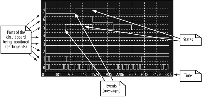
A logic analyzer captures a sequence of events as they occur on an electronic circuit board. A readout from a logic analyzer (such as the one shown in Figure 9-1) will typically show the time at which different parts of the circuit board are in particular states and the electronic signals that will trigger changes in those states.

Timing diagrams perform a similar job for the participants within your system. On a timing diagram, events are the logic analyzer’s signals, and the states are the states that a participant is placed in when an event is received. The similarities between a timing diagram and a logic analyzer are apparent when you compare Figure 9-1 with Figure 9-2, which gives a sneak preview of how a complete timing diagram looks. This example was taken from UML 2.0 in a Nutshell (O’Reilly).

Figure 9-2. Compare this simple yet complete timing diagram for a mail server with the logic analyzer in Figure 9-1

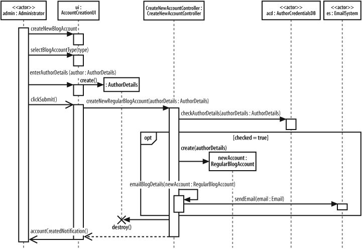
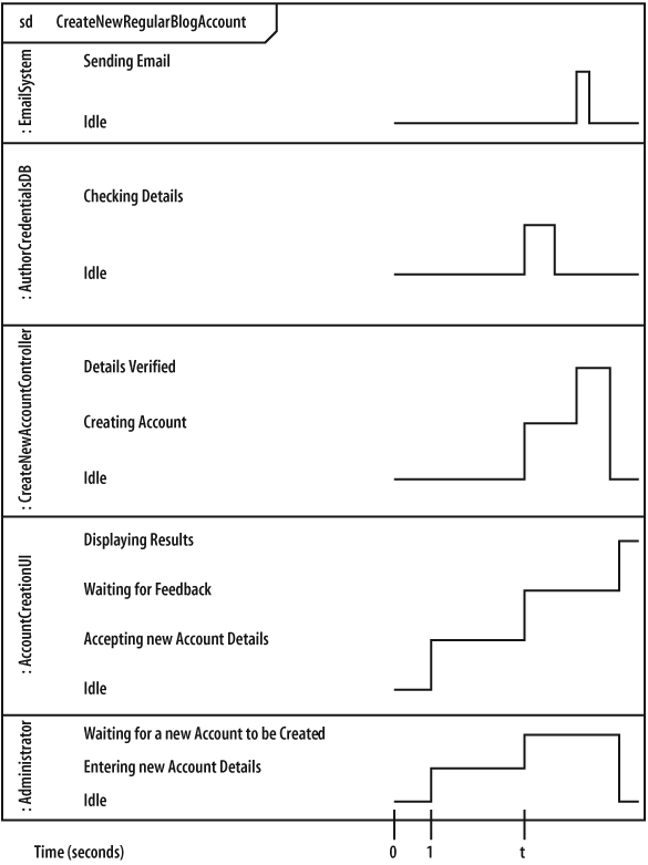
Let’s assemble a timing diagram from scratch. We’re going to work from the same example used in the communication and sequence diagram chapters, the Create a new Regular Blog Account interaction, shown in Figure 9-3.

Figure 9-3. A sequence diagram contains very little, if any, information about timing, and its main focus is the order of events within an interaction

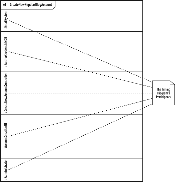
First, you need to create a timing diagram that incorporates all of the participants involved in the Create a new Regular Blog Account interaction, as shown in Figure 9-4.

The full participant names have been left out of Figure 9-4 to keep the diagram’s size manageable, although you could equally have included the full <name>:<type> format for the title of a participant.

Another feature that is missing from Figure 9-4 is the participants that are created and destroyed within the life of the interaction: the :AuthorDetails and :RegularBlogAccountparticipants. Details of these participants have been left out because timing diagrams focus on timing in relation to state changes. Apart from being created and/or destroyed, the :AuthorDetails and :RegularBlogAccount participants do not have any complicated state changes; therefore, they are omitted because they would not add anything of interest to this particular diagram.

Figure 9-4. The names of the main participants involved in an interaction are written vertically on the lefthand side of a timing diagram

During an interaction, a participant can exist in any number of states. A participant is said to be in a particular state when it receives an event (such as a message). The participant can then be said to be in that state until another event occurs (such as the return of that message). See the "Events and Messages" section later in this chapter for an explanation of how events and messages are applied to timing diagrams.

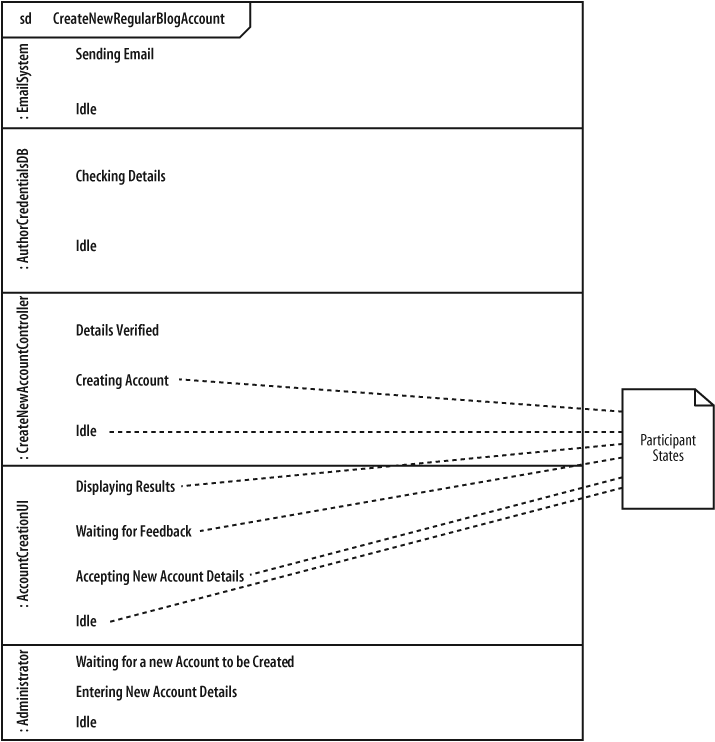
States on a timing diagram are placed next to their corresponding participant, as shown in Figure 9-5.

Figure 9-5. States are written horizontally on a timing diagram and next to the participant that they are associated with

For a type of diagram that is actually called a “timing” diagram, it might seem a little strange that we haven’t yet mentioned time. So far, we’ve just been setting the stage, adding participants and the states that they can be put in, but to really model the information that’s important to a timing diagram, it’s now time to add time (pun intended).

Exact Time Measurements and Relative Time Indicators

Time on a timing diagram runs from left to right across the page, as shown in Figure 9-6.

Figure 9-6. Time measurements are placed on a timing diagram as a ruler along the bottom of the page

Time measurements can be expressed in a number of different ways; you can have exact time measurements , as shown in Figure 9-6, or relative time indicators , as shown in Figure 9-7.

Figure 9-7. Relative time indicators are particularly useful when you have timing considerations such as “ParticipantA will be in State1 for half of the time that ParticipantB is in State2”

In a timing diagram, t represents a point in time that is of interest. You don’t know exactly when it will happen because it may happen in response to a message or event, but t is a way to refer to that moment without knowing exactly when it is. With t as a reference, you can then specify time constraints relative to that point t.

Adding time to the diagram we’ve been putting together so far is tricky because we don’t have any concrete timing information in the original requirement. See the "Timing Constraints in System Requirements" section earlier in this chapter if you need a quick reminder as to what the extended Requirement A.2 states.

However, we still need to apply the constraints mentioned in Requirement A.2, so some measure of relative time represented by t is shown in Figure 9-8.

Figure 9-8. The timing constraints are a blend of exact and relative timings

In this figure, the initial stages of the interaction are simply measured as seconds, and the single t value represents a single second wherever it is mentioned on any further timing constraints on the diagram. See the "Timing Constraints" section later in this chapter for more on how the value t can be used on a timing diagram.

Now that you have added time to the timing diagram (fancy that!), you can show what state a participant is in at any given time. If you take a look back at Figure 9-6 and Figure 9-7, you can already see how participant’s current state is indicated: with a horizontal line that is called the state-line.

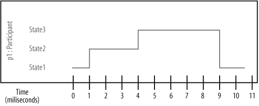
At any given time in the interaction, a participant’s state-line is aligned with one of the participant’s states (see Figure 9-9).

Figure 9-9. In this example, p1:Participant’s state-line indicates that it is in State1 for 1 unit of time, State2 for three units of time, and State3 for roughly five units of time (before returning to State1 at the end of the interaction)

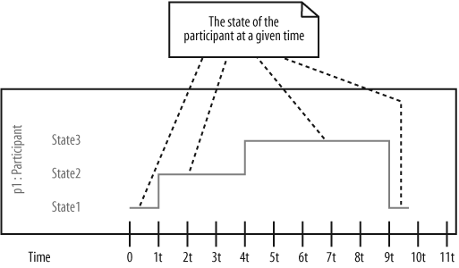
Figure 9-10 shows how the Create a new Regular Blog Account timing diagram is updated to show the state of each participant at a given time during the interaction.

That’s all there is to showing that a participant is in a specific state at a given time. Now it’s time to look at why a participant changes states in the first place, which leads us neatly to events and messages.

Figure 9-10. Each of the participants needs to have a corresponding state-line to indicate their state at any given point in time

Participants change state on a timing diagram in response to events. These events might be the invocation of a message or they might be something else, such as a message returning after it has been invoked. The distinction between messages and events is not as important on a timing diagram as it is on sequence diagrams. The important thing to remember is that whatever the event is, it is shown on a timing diagram to trigger a change in the state of a participant.

An event on a timing diagram is shown as an arrow from one participant’s state-line—the event source—to another participant’s state-line—the event receiver (as shown in Figure 9-11).

Figure 9-11. Events on a timing diagram can even have their own durations, as shown by event1 taking 1 unit of time from invocation by p1:Participant1 and reception by p2:Participant2

Adding events to the timing diagram is actually quite a simple task, because you have the sequence diagram from Figure 9-3 to refer to. The sequence diagram already shows the messages that are passed between participants, so you can simply add those messages to the timing diagram, as shown in Figure 9-12.

Up until this point, you have really only been establishing the foundation of a timing diagram. Participants, states, time, and events and messages are the backdrop against which you can start to model the information that is really important to a timing diagram—timing constraints .

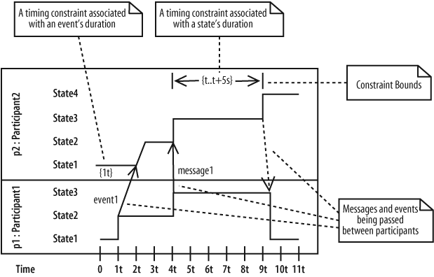
Timing constraints describe in detail how long a given portion of an interaction should take. They are usually applied to the amount of time that a participant should be in a particular state or how long an event should take to be invoked and received, as shown in Figure 9-13. By applying constraints to this timing diagram, the duration of event1 must be less than one value of the relative measure t, and p2:Participant2 should be in State4 for a maximum of five seconds.

Figure 9-12. Participant state changes make much more sense when you can see the events that cause them

Timing Constraint Formats

A timing constraint can be specified in a number of different ways, depending on the information your are trying to model. Table 9-1 shows some common examples of timing constraints.

Figure 9-13. Timing constraints can be associated with an event or a state and may or may not be accompanied by constraint boundary arrows

Table 9-1. Different ways of specifying a timing constraint

Timing Constraint	Description
{t..t+5s}	The duration of the event or state should be 5 seconds or less.
{<5s}	The duration of the event or state should be less than 5 seconds. This is a slightly less formal than {t..t+5s}, but an equivalent notation.
{>5s, <10s}	The duration of the event or state should be greater than 5 seconds, but less than 10 seconds.
{t}	The duration of the event or state should be equal to the value of t. This is a relative measure, where t could be any value of time.
{t..t*5}	The duration of the event or state should be the value of t multiplied 5 times. This is another relative measure (t could be any value of time).

Applying Timing Constraints to States and Events

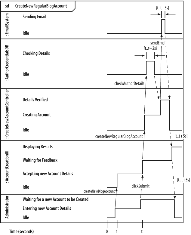
At the beginning of this chapter, we extended Requirement A.2 to specify some timing considerations. Requirement A.2’s timing considerations can now be added to the timing diagram as timing constraints. Figure 9-14 completes the Create a new Regular Blog Account timing diagram, capturing Requirement A.2’s timing considerations by applying constraints to the relevant states.

As you can see from Figure 9-14, applying the 5 seconds per new regular blog account creation timing constraint is not a straightforward job since it affects several different nested interactions between participants. This is where the skill of the modeler comes into play on a timing diagram; you need to decide which events or states need to be allocated portions of the available five seconds so each participant can do its job (and get those allocations right).

Figure 9-14. From when the :Administrator clicks on submit until the point at which the system has created a new account, no more than five seconds have passed

Where you arrange participants on a timing diagram does not at first appear to be very important. However, as you add more details to your diagram in the form of events and timing information, you’ll soon discover that the place where a participant is located on the timing diagram can cause problems if you haven’t thought about it carefully enough (see Figure 9-15).

Figure 9-15. The bottom diagram is harder to read, and details are beginning to obscure one another

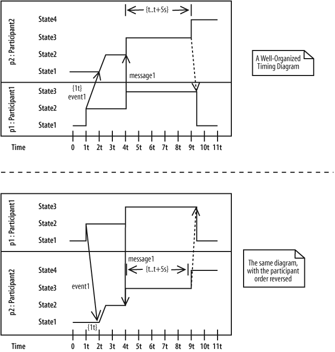
If you’re lucky and you already have a sequence diagram for an interaction, then there is an easy rule of thumb to get you started when arranging participants for the first time on a timing diagram. Simply take the order of the participants as they appear across the top of the page on a sequence diagram and flip the list of participant names 90 degrees counterclockwise, as shown in Figure 9-16. If your sequence diagram is well-organized, then you should now have a good candidate order for placing the participants on your timing diagram.

Figure 9-16. Rotating a sequence diagram’s major participant’s 90 degrees counterclockwise is an easy way to get an initial placement for your timing diagram’s participants

Real estate on a UML diagram is almost always at a premium. In previous versions of UML, sequence diagrams were known as being the hardest diagram to manage when modeling a complex interaction. Although timing diagrams are not going to steal the sequence diagram’s crown in this respect, the regular timing diagram notation shown in this chapter so far doesn’t scale particularly well when you need to model a large number of different states.

The Create a new Regular Blog Account interaction’s timing diagram, as shown in Figure 9-14, is actually a fairly simple example. However, you might already be beginning to grasp how large a timing diagram can get—at least vertically—for anything more than a trivial interaction that includes a small number of states. A good UML 2.0 tool will help you work with and manage large timing diagrams, but there is only so much a tool can really do.

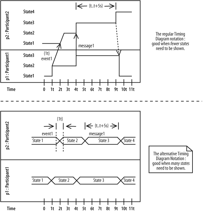
The developers of UML 2.0 realized this problem and created an alternative, simpler notation for when you have an interaction that contains a large number of states, shown in Figure 9-17.

When you look closely at the alternative timing diagram notation, things are not dramatically different from the regular notation. The notation for participants and time hasn’t changed at all. The big change between the regular timing diagram notation and the alternative is in how states and state changes are shown.

The regular timing diagram notation shows states as a list next to the relevant participant. A state-line is then needed to show what state a participant is in at a given time. Unfortunately, if a participant has many different states, then the amount of space needed to model a participant on the timing diagram will grow quickly.

The alternative notation fixes this problem by removing the vertical list of different states. It places a participant’s states directly at the point in time when the participant is in that state. Therefore, the state-line is no longer needed, and all of the states for a particular participant can be placed in a single line across the diagram.

To show that a participant changes state because of an event, a cross is placed between the two states and the event that caused the state change is written next to the cross. Timing constraints can then be applied in much the same way as regular notations.

Bringing the subject of timing diagrams to a close, Figure 9-18 shows the alternate timing diagram notation in a practical setting: modeling the Create a new Regular Blog Account interaction.

Figure 9-17. The top diagram’s notation should be familiar to you, but the diagram at the bottom uses the new alternative timing diagram notation

Figure 9-18. Even though there are not many states in this interaction, you can begin to see how the alternate notation is more compact and manageable in a situation where there are many states per participant

The concept of an object’s state is integral to timing diagrams since they show states of an object at particular times. State machine diagrams show in detail the states of an object and triggers that cause state changes. Both diagram types are very important to models of real-time and embedded systems. State machine diagrams are covered in Chapter 14.