Let’s look at the basic elements of activity diagrams by modeling a process encountered earlier in the book—the steps in the blog account creation use case. Table 3-1 contains the Create a new Blog Account use case description (originally Table 2-1). The Main Flow and Extension sections describe steps in the blog account creation process.

Figure 3-2 shows this blog account creation process in activity diagram notation. An activity diagram is useful here because it helps you to better visualize a use case’s steps (compared to the table notation in the use case description), especially the branching steps that depend on whether the author is verified.

In Figure 3-2, the activity is launched by the initial node , which is drawn as a filled circle. The initial node simply marks the start of the activity. At the other end of the diagram, the activity final node, drawn as two concentric circles with a filled inner circle, marks the end of the activity.

Figure 3-2. Activity diagrams model dynamic behavior with a focus on processes; the basic elements of activity diagrams are shown in this blog account creation process

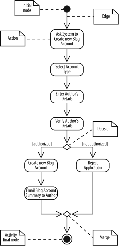
In between the initial node and the activity final node are actions , which are drawn as rounded rectangles. Actions are the important steps that take place in the overall activity, e.g., Select Account Type, Enter Author's Details, and so on. An action could be a behavior performed, a computation, or any key step in the process.

The flow of the activity is shown using arrowed lines called edges or paths. The arrowhead on an activity edge shows the direction of flow from one action to the next. A line going into a node is called an incoming edge, and a line exiting a node is called an outgoing edge. Edges string the actions together to determine the overall activity flow: first the initial node becomes active, then Ask System to create new Blog Account, and so on.

The first diamond-shaped node is called a decision, analogous to an if-else statement in code. Notice that there are two outgoing edges from the decision in Figure 3-2, each labeled with Boolean conditions. Only one edge is followed out of the decision node depending on whether the author is authorized. The second diamond-shaped node is called a merge. A merge node combines the edges starting from a decision node, marking the end of the conditional behavior.

The word “flow” was mentioned several times previously and you may ask—what’s flowing? The answer depends on the context. Typically, it’s the flow of control from one action to the next: one action executes to completion, then gives up its control to the next action. In later sections you’ll see that, along with control, objects can flow through an activity.

Actions are active steps in the completion of a process. An action can be a calculation, such as Calculate Tax, or a task, such as Verify Author's Details.

The word “activity” is often mistakenly used instead of “action” to describe a step in an activity diagram, but they are not the same. An activity is the process being modeled, such as washing a car. An action is a step in the overall activity, such as Lather, Rinse, and Dry.

The actions in this simple car-washing activity are shown in Figure 3-3.

Figure 3-3. Capturing the three actions—Lather, Rinse, and Dry—that make up washing a car in an activity diagram

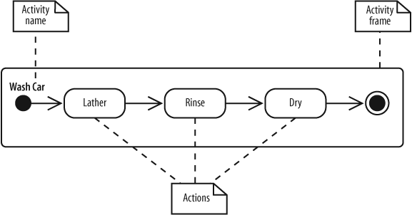
In Figure 3-3, the entire activity is enclosed within the rounded rectangle called an activity frame . The activity frame is used to contain an activity’s actions and is useful when you want to show more than one activity on the same diagram. Write the name of the activity in the upper left corner.

The activity frame is optional and is often left out of an activity diagram, as shown in the alternative Wash Car activity in Figure 3-4.

Figure 3-4. The activity frame can be omitted

Although you lose the name of the activity being displayed on the diagram itself, it is often more convenient to leave out the activity frame when constructing a simple activity diagram.

Decisions are used when you want to execute a different sequence of actions depending on a condition. Decisions are drawn as diamond-shaped nodes with one incoming edge and multiple outgoing edges, as shown in Figure 3-5.

Figure 3-5. Only one edge is followed after a decision node

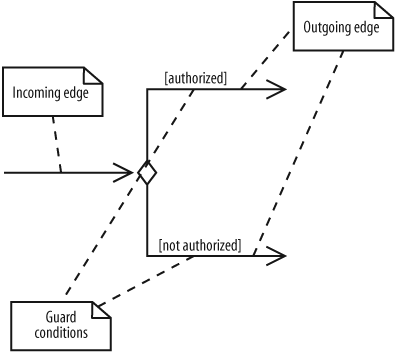
Each branched edge contains a guard condition written in brackets. Guard conditions determine which edge is taken after a decision node.

They are statements that evaluate to true or false, for example:

The branched flows join together at a merge node, which marks the end of the conditional behavior started at the decision node. Merges are also shown with diamond-shaped nodes, but they have multiple incoming edges and one outgoing edge, as shown in Figure 3-6.

Figure 3-6. If the input value of age is 1200, then the Notify Blog Entry too long action is performed

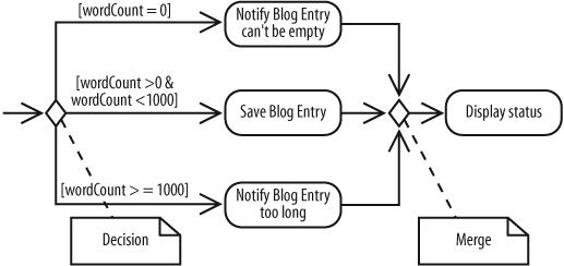
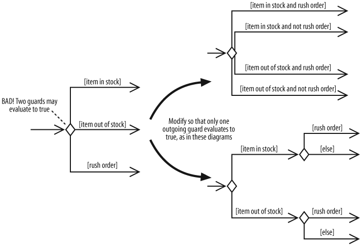
Activity diagrams are clearest if the guards at decision nodes are complete and mutually exclusive. Figure 3-7 shows a situation in which the paths are not mutually exclusive.

If an item is in stock and the order is a rush order, then two guards evaluate to true. So which edge is followed? According to the UML specifications, if multiple guards evaluate to true, then only one edge is followed and that choice is out of your control unless you specify an order. You can avoid this complicated situation by making guards mutually exclusive.

The other situation to avoid is incomplete guards. For example, if Figure 3-7 had no guard covering out of stock items, then an out of stock item can’t follow any edge out of the decision node. This means the activity is frozen at the decision node. Modelers sometimes leave off guards if they expect a situation not to occur (or if they want to defer thinking about it until later), but to minimize confusion, you should always include a guard to cover every possible situation. If it’s possible in your activity, it’s helpful to label one path with else, as shown in Figure 3-7, to make sure all situations are covered.

Figure 3-7. Beware of diagrams where multiple guards evaluate to true

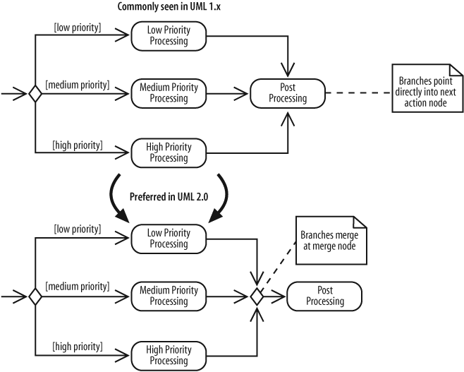
If you’re coming from a UML 1.x background, it may not seem necessary to show merge nodes. In UML 1.x, it was common to see multiple edges starting at a decision node flow directly into an action, as shown in the top part of Figure 3-8. This meant the flows were merged implicitly.

As of UML 2.0, when multiple edges lead directly into an action, all incoming flows are waited on before proceeding. But this doesn’t make sense because only one edge is followed out of a decision node. You can avoid confusing your reader by explicitly showing merge nodes.

Consider a computer assembly workflow that involves the following steps:

So far we’ve covered enough activity diagram notation to model this workflow sequentially. But suppose the entire workflow can by sped up by preparing the case and the motherboard at the same time since these actions don’t depend on each other. Steps that occur at the same time are said to occur concurrently or in parallel.

Figure 3-8. In UML 2.0, it’s better to be as clear as possible and to show merge nodes

You represent parallel actions in activity diagrams by using forks and joins, as shown in the activity diagram fragment in Figure 3-9.

Figure 3-9. Both outgoing paths are followed at the fork, in contrast with decision nodes, where only one outgoing path is taken

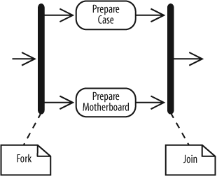
After a fork in Figure 3-9, the flow is broken up into two or more simultaneous flows, and the actions along all forked flows execute. In Figure 3-9, Prepare Case and Prepare Motherboard begin executing at the same time.

The join means that all incoming actions must finish before the flow can proceed past the join. Forks and joins look identical—they are both drawn with thick bars—but you can tell the difference because forks have multiple outgoing flows, whereas joins have multiple incoming flows.

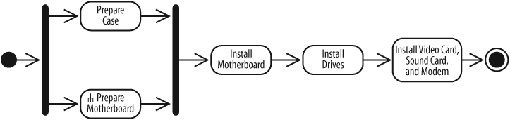
Figure 3-10 completes the activity diagram for the computer assembly workflow.

Figure 3-10. The computer assembly workflow demonstrates how forks and joins work in a complete activity diagram

When actions occur in parallel, it doesn’t necessarily mean they will finish at the same time. In fact, one task will most likely finish before the other. However, the join prevents the flow from continuing past the join until all incoming flows are complete. For example, in Figure 3-10 the action immediately after the join—Install Motherboard—executes only after both the Prepare Case and Prepare Motherboard actions finish.

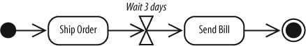
Sometimes time is a factor in your activity. You may want to model a wait period, such as waiting three days after shipping an order to send a bill. You may also need to model processes that kick off at a regular time interval, such as a system backup that happens every week.

Time events are drawn with an hourglass symbol. Figure 3-11 shows how to use a time event to model a wait period. The text next to the hourglass—Wait 3 Days—shows the amount of time to wait. The incoming edge to the time event means that the time event is activated once. In Figure 3-11, the bill is sent only once—not every three days.

Figure 3-11. A time event with an incoming edge represents a timeout

A time event with no incoming flows is a recurring time event, meaning it’s activated with the frequency in the text next to the hourglass. In Figure 3-12, the progress bar is updated every second.

Figure 3-12. A time event with no incoming flows models a repeating time event

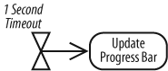
Notice that there is no initial node in Figure 3-12; a time event is an alternate way to start an activity. Use this notation to model an activity that is launched periodically.

As detail is added to your activity diagram, the diagram may become too big, or the same sequence of actions may occur more than once. When this happens, you can improve readability by providing details of an action in a separate diagram, allowing the higher level diagram to remain less cluttered.

Figure 3-13 shows the computer assembly workflow from Figure 3-10, but the Prepare Motherboard action now has an upside-down pitchfork symbol indicating that it is a call activity node. A call activity node calls the activity corresponding to its node name. This is similar to calling a software procedure.

Figure 3-13. Rather than cluttering up the top-level diagram with details of the Prepare Motherboard action, details are provided in another activity diagram

The Prepare Motherboard node in Figure 3-13 invokes the Prepare Motherboard activity in Figure 3-14. You associate a call activity node with the activity it invokes by giving them the same name. Call activities essentially break an action down into more details without having to show everything in one diagram.

Figure 3-14. The Prepare Motherboard activity elaborates on the motherboard preparation process

The Prepare Motherboard activity diagram has its own initial and activity final nodes. The activity final node marks the end of Prepare Motherboard, but it doesn’t mean the calling activity is complete. When Prepare Motherboard terminates, control is returned to the calling activity, which proceeds as normal. This is another reason call activities resemble invoked software procedures.

Sometimes data objects are an important aspect of the process you’re modeling. Suppose your company decides to sell the CMS as a commercial product, and you want to define a process for approving incoming orders. Each step in the order approval process will need information about the order, such as the payment information and transaction cost. This can be modeled in your activity diagram with an Order object, which contains the order information needed by the steps. Activity diagrams offer a variety of ways to model objects in your processes.

Showing Objects Passed Between Actions

In activity diagrams, you can use object nodes to show data flowing through an activity. An object node represents an object that is available at a particular point in the activity, and can be used to show that the object is used, created, or modified by any of its surrounding actions.

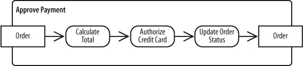
An object node is drawn with a rectangle, as shown in the order approval process in Figure 3-15. The Order object node draws attention to the fact that the Order object flows from the Receive Order Request action to the Approve Payment action.

Figure 3-15. The Order object node emphasizes that it is important data in this activity and shows which actions interact with it

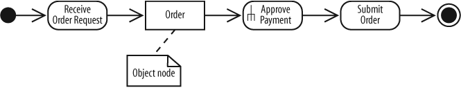
See "Sending and Receiving Signals" for a more precise way of modeling the Receive Order Request action—as a receive signal node.

Showing Action Inputs and Outputs

Figure 3-16 shows a different perspective on the previous activity using pins . Pins show that an object is input to or output from an action.

An input pin means that the specified object is input to an action. An output pin means that the specified object is output from an action. In Figure 3-16, an Order object is input to the Approve Payment action and an Order object is output from the Receive Order Request action.

Figure 3-16. Pins in this change request approval process allow finer-grained specification of input and output parameters

Figures 3-15 and 3-16 show similar situations, but pins are good at emphasizing that an object is required input and output, whereas an object node simply means that the object is available at that particular point in the activity. However, object nodes have their own strength; they are good at emphasizing the flow of data through an activity.

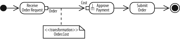
If the Approve Payment action needs only parts of the Order object—not the whole object—you can use a transformation to show which parts are needed. Transformations allow you to show how the output from one action provides the input to another action.

Figure 3-17 specifies that the Approve Payment action requires the Cost object as input and shows how this data is obtained from the Order object using the transformation specified in a note.

Figure 3-17. Transformations show where input parameters come from

Showing How Objects Change State During an Activity

You can also show an object changing state as it flows through an activity. Figure 3-18 shows that the Order object’s state is pending before Approve Payment and changes to approved afterward. The state is shown in brackets.

Figure 3-18. The focus of this diagram is the change of state of the Order object throughout the order approval process

Showing Input to and Output from an Activity

In addition to acting as inputs to and outputs from actions, object nodes can be inputs to and outputs from an activity. Activity inputs and outputs are drawn as object nodes straddling the boundary of the activity frame, as shown in Figure 3-19. This notation is useful for emphasizing that the entire activity requires input and provides output.

Figure 3-19 shows the Order object as input and output for the Approve Payment activity. When input and output parameters are shown, the initial node and activity final node are omitted from the activity.

Figure 3-19. Object nodes can be used to emphasize input to and output from an activity

Activities may involve interactions with external people, systems, or processes. For example, when authorizing a credit card payment, you need to verify the card by interacting with an approval service provided by the credit card company.

In activity diagrams, signals represent interactions with external participants. Signals are messages that can be sent or received, as in the following examples:

A receive signal has the effect of waking up an action in your activity diagram. The recipient of the signal knows how to react to the signal and expects that a signal will arrive at some time but doesn’t know exactly when. Send signals are signals sent to an external participant. When that external person or system receives the message, it probably does something in response, but that isn’t modeled in your activity diagram.

Figure 3-20 refines the steps in Figure 3-19 to show that the credit card approval action requires interaction with external software. The send signal node shows that a signal is sent to an outside participant. In this example, the signal is a credit card approval request. Signals are sent asynchronously, meaning the activity does not wait for the response but moves immediately to the next action after the signal is sent.

Figure 3-20. Send and receive signal nodes show interactions with external participants

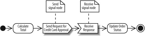
The receive signal node shows that a signal is received from an external process. In this case, the system waits for a response from the credit card company. At a receive signal node, the action waits until a signal is received and proceeds only when a signal is received.

When you see a receive signal node with no incoming flows, it means that the node is always waiting for a signal when its containing activity is active. In the case of Figure 3-21, the activity is launched every time an account request signal is received.

Figure 3-21. Starting an activity with a receive signal node: the receive signal node replaces the usual initial node

This differs from a receive signal node with an incoming edge, such as the Receive Response node in Figure 3-20; a receive signal node with an incoming edge only starts waiting when the previous action is complete.

The simplest and most common way to start an activity is with a single initial node; most of the diagrams you’ve seen so far in this chapter use this notation. There are other ways to represent the start of an activity that have special meanings:

To specify that an activity starts as a result of being woken up by a signal, use a receive signal node instead of an initial node. Inside the receive signal, node you specify what type of event starts the activity. Figure 3-21 shows an activity starts upon receipt of an order.

The end nodes in this chapter haven’t been very interesting so far; in fact, they haven’t acted as much more than end markers. In the real world, you can encounter more complex endings to processes, including flows that can be interrupted and flows that end without terminating the overall activity.

Interrupting an Activity

Figure 3-21 above shows a typical activity diagram with a simple ending. Notice there’s only one path leading into the activity final node; every action in this diagram gets a chance to finish.

Sometimes you need to model that a process can be terminated by an event. This could happen if you have a long running process that can be interrupted by the user. Or, in the CMS order handling activity, you may need to account for an order being canceled. You can show interruptions with interruption regions .

Draw an interruption region with a dashed, rounded rectangle surrounding the actions that can be interrupted along with the event that can cause the interruption. The interrupting event is followed by a line that looks like a lightning bolt. Figure 3-22 extends Figure 3-21 to account for the possibility that an order might be canceled.

Figure 3-22. Interruption region showing a process that can be interrupted

In Figure 3-22, if a cancellation is received while Process Order is active, Process Order will be interrupted and Cancel Order will become active. Cancellation regions are relevant only to the contained actions. If a cancellation is received while Ship Order is active, Ship Order won’t be interrupted since it’s not in the cancellation region.

Tip

Sometimes you’ll see activity diagrams with multiple activity final nodes instead of multiple flows into a single activity final node. This is legal and can help detangle lines in a diagram that has many branches. But activity diagrams are usually easier to understand if they contain a single activity final node.

Ending a Flow

A new feature of UML 2.0 is the ability to show that a flow dies without ending the whole activity. A flow final node terminates its own path—not the whole activity. It is shown as a circle with an X through it, as in Figure 3-23.

Figure 3-23. A flow final node terminates only its own path—not the whole activity

Figure 3-23 shows a search engine for the CMS with a two-second window to generate the best possible search results. When the two-second timeout occurs, the search results are returned, and the entire activity ends, including the Improve Search Results action. However, if Improve Search Results finishes before the two-second timeout, it will not stop the overall activity since its flow ends with a flow final node.

Warning

Be careful when using a flow final node after a fork. As soon as the activity final node is reached, all other actions in the activity (including the ones before the final node) terminate. If you want all forked actions to run to completion, make sure to add a join.

Activities may involve different participants, such as different groups or roles in an organization or system. The following scenarios require multiple participants to complete the activity (participant names are italicized):

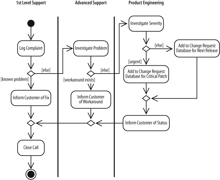
You use partitions to show which participant is responsible for which actions. Partitions divide the diagram into columns or rows (depending on the orientation of your activity diagram) and contain actions that are carried out by a responsible group. The columns or rows are sometimes referred to as swimlanes.

Figure 3-24 shows a technical support process involving three types of participants: 1st level Support, Advanced Support, and Product Engineering.

Figure 3-24. Partitions help organize this activity diagram by clarifying responsible parties

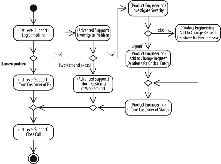
You can also show responsibility by using annotations. Notice that there are no swimlanes; instead, the name of the responsible party is put in parentheses in the node, shown in Figure 3-25. This notation typically makes your diagram more compact, but it shows the participants less clearly than swimlanes.

Figure 3-25. Annotations can be used instead of swimlanes as a way of showing responsibility directly in the action

Activity diagrams have many additional symbols to model a wide range of processes. The following sections feature some convenient shortcuts for simplifying your activity diagrams. See UML 2.0 in a Nutshell (O’Reilly) for a more complete list.

Connectors

If your activity diagram has a lot of actions, you can end up with long, crossing lines, which make the diagram hard to read. This is where connectors can help you out.

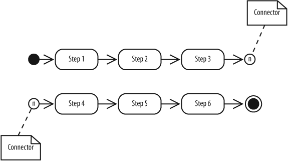
Connectors help untangle your diagrams, connecting edges with symbols instead of explicit lines. A connector is drawn as a circle with its name written inside. Connectors are typically given single character names. In Figure 3-26, the connector name is n.

Connectors come in pairs: one has an incoming edge and the other has an outgoing edge. The second connector picks up where the first connector left off. So the flow in Figure 3-26 is the same as if Step 3 had an edge leading directly into Step 4.

Figure 3-26. Connectors can improve the readability of a large activity diagram

Warning

Be careful with connectors: if you use too many different connectors in one diagram, the reader may have a hard time pairing them.

Expansion Regions

Expansion regions show that actions in a region are performed for each item in an input collection. For example, an expansion region could be used to model a software function that takes a list of files as input and searches each file for a search term.

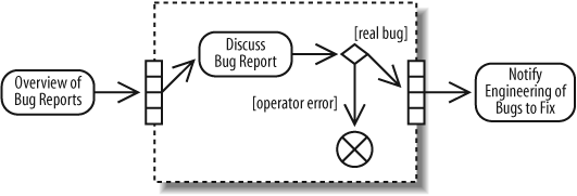
Draw an expansion region as a large rounded rectangle with dashed lines and four aligned boxes on either side. The four boxes represent input and output collections (but they don’t imply that the collection size is four). Figure 3-27 shows that the bug report is discussed for each bug report in an input collection. If it’s a real bug, then the activity proceeds; otherwise the bug is discarded and the flow for that input ends.

Figure 3-27. The actions in an expansion region are performed for each item in a collection

Sequence and communication diagrams are other UML diagrams that can model the dynamic behavior of your system. These diagrams focus on showing detailed interactions, such as which objects are involved in an interaction, which methods are invoked, and the sequence of events. Sequence diagrams can be found in Chapter 7. Communication diagrams are covered in Chapter 8.

If you haven’t already, it’s also worth reading Chapter 2 on use cases because activity diagrams offer a great way of showing a visual representation of a use case’s flow.