
Chapter 15. Modeling Your Deployed System: Deployment Diagrams
If you’ve been applying the UML techniques shown in earlier chapters of this book, then you’ve seen all but one view of your system. That missing piece is the physical view. The physical view is concerned with the physical elements of your system, such as executable software files and the hardware they run on.
UML deployment diagrams show the physical view of your system, bringing your software into the real world by showing how software gets assigned to hardware and how the pieces communicate (see Figure 15-1).

Tip
The word system can mean different things to different people; in the context of deployment diagrams, it means the software you create and the hardware and software that allow your software to run.
Deploying a Simple System
Let’s start by showing a deployment diagram of a very simple system. In this simplest of cases, your software will be delivered as a single executable file that will reside on one computer.
To show computer hardware, you use a node, as shown in Figure 15-2.
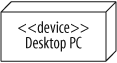
This system contains a single piece of hardware—a Desktop PC. It’s labeled with the stereotype <<device>> to specify that this is a hardware node.
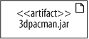
Now, you need to model the software that runs on the hardware. Figure 15-3 shows a simple software artifact (see "Deployed Software: Artifacts,” next), which in this case is just a JAR file named 3dpacman.jar, containing a 3D-Pacman application.
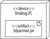
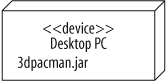
Finally, you need to put these two pieces together to complete the deployment diagram of your system. Draw the artifact inside the node to show that a software artifact is deployed to a hardware node. Figure 15-4 shows that 3dpacman.jar runs on a Desktop PC.
But is it really complete? Don’t you need to model the Java Virtual Machine (JVM) because without it, your code wouldn’t execute? What about the operating system; isn’t that important? The answer, unfortunately, is possibly.
Your deployment diagrams should contain details about your system that are important to your audience. If it is important to show the hardware, firmware, operating system, runtime environments, or even device drivers of your system, then you should include these in your deployment diagram. As the rest of this chapter will show, deployment diagram notation can be used to model all of these types of things. If there’s a feature of your system that’s not important, then it’s not worth adding it to your diagram since it could easily clutter up or distract from those features of your design that are important.
Deployed Software: Artifacts
The previous section showed a sneak preview of some of the notation that can be used to show the software and hardware in a deployed system. The 3dpacman.jar software was deployed to a single hardware node. In UML, that JAR file is called an artifact.
Artifacts are physical files that execute or are used by your software. Common artifacts you’ll encounter include:
Executable files, such as .exe or .jar files
Library files, such as .dlls (or support .jar files)
Source files, such as .java or .cpp files
Configuration files that are used by your software at runtime, commonly in formats such as .xml, .properties, or .txt
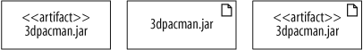
An artifact is shown as a rectangle with the stereotype <<artifact>>, or the document icon in the upper right hand corner, or both, as shown in Figure 15-5. For the rest of the book, an artifact will be shown with both the stereotype <<artifact>> and the document icon.
Deploying an Artifact to a Node
An artifact is deployed to a node, which means that the artifact resides on (or is installed on) the node. Figure 15-6 shows the 3dpacman.jar artifact from the previous example deployed to a Desktop PC hardware node by drawing the artifact symbol
inside the node.

You can model that an artifact is deployed to a node in two other ways. You can also draw a dependency arrow from the artifact to the target node with the stereotype <<deploy>>, as shown in Figure 15-7.

When you’re pressed for space, you might want to represent the deployment by simply listing the artifact’s name inside the target node, as shown in Figure 15-8.
All of these methods show the same deployment relationship, so here are some guidelines for picking a notation.
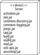
Listing the artifacts (without the artifact symbol) can really save space if you have a lot of artifacts, as in Figure 15-9. Imagine how big the diagram would get if you drew the artifact symbol for each artifact.
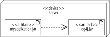
But be careful; by listing your artifacts, you cannot show dependencies between artifacts. If you want to show that an artifact uses another artifact, you have to draw the artifact symbols and a dependency arrow connecting the artifacts, as shown in Figure 15-10.
Tying Software to Artifacts
When designing software, you break it up into cohesive groups of functionality, such as components or packages, which eventually get compiled into one or more files—or artifacts. In UML-speak, if an artifact is the physical actualization of a component, then the artifact manifests that component. An artifact can manifest not just components but any packageable element, such as packages and classes.
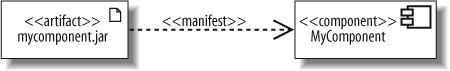
The manifest relationship is shown with a dependency arrow from the artifact to the component with the stereotype <<manifest>>, as shown in Figure 15-11.
Since artifacts can then be assigned to nodes, the manifest relationship provides the missing link in modeling how your software components are mapped to hardware. However, linking a component to an artifact to a node can result in a cluttered diagram, so it’s common to show the manifest relationships separate from the deployment relationships, even if they’re on the same deployment diagram.
Tip
You can also show the manifest relationship in component diagrams by listing the artifacts manifesting a component within the component symbol, as discussed in Chapter 12.
If you’re familiar with earlier versions of UML, you may be tempted to model a component running on hardware by drawing the component symbol inside the node. As of UML 2.0, artifacts have nudged components toward a more conceptual interpretation, and now artifacts represent physical files.
However, many UML tools aren’t fully up to date with the UML 2.0 standard, so your tool may still use the earlier notation.
What Is a Node?
You’ve already seen that you can use nodes to show hardware in your deployment diagram, but nodes don’t have to be hardware. Certain types of software—software that provides an environment within which other software components can be executed—are nodes as well.
A node is a hardware or software resource that can host software or related files. You can think of a software node as an application context; generally not part of the software you developed, but a third-party environment that provides services to your software.
The following items are reasonably common examples of hardware nodes:
Server
Desktop PC
Disk drives
The following items are examples of execution environment nodes:
Operating system
J2EE container
Web server
Application server
Warning
Software items such as library files, property files, and executable files that cannot host software are not nodes—they are artifacts (see "Deployed Software: Artifacts,” earlier in the chapter).
Hardware and Execution Environment Nodes
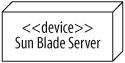
A node is drawn as a cube with its type written inside, as shown in Figure 15-12. The stereotype <<device>> emphasizes that it’s a hardware node.
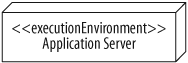
Figure 15-13 shows an Application Server node. Those familiar with enterprise software development will recognize this as a type of execution environment since it’s a software environment that provides services to your application. The stereotype <<executionEnvironment>> emphasizes that this node is an execution environment.
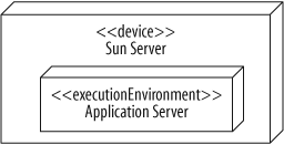
Execution environments do not exist on their own—they run on hardware. For example, an operating system needs computer hardware to run on. You show that an execution environment resides on a particular device by placing the nodes inside one another, nesting them as shown in Figure 15-14.
It’s not strictly necessary in UML 2.0 to distinguish device nodes from execution environment nodes, but it’s a good habit to get into because it can clarify your model.
Tip
Want more variety? If you’re using a profile (discussed in Appendix B), you can apply node stereotypes that are more relevant to your domain, such as <<J2EE Container>>. These new node types can be specified in your profile as a special kind of execution environment.
Showing Node Instances
There are times when your diagram includes two nodes of the same type, but you want to draw attention to the fact that they are actually different instances. You can show an instance of a node by using the name : type notation as shown in Figure 15-15.
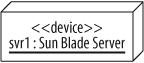
Figure 15-16 shows how two nodes of the same type can be modeled. The nodes in this example, svr1 and svr2, are assigned different types of traffic from a load balancer (a common situation in enterprise systems).

Communication Between Nodes
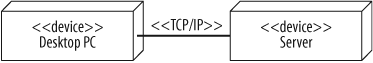
To get its job done, a node may need to communicate with other nodes. For example, a client application running on a desktop PC may retrieve data from a server using TCP/IP.
Communication paths are used to show that nodes communicate with each other at runtime. A communication path is drawn as a solid line connecting two nodes. The type of communication is shown by adding a stereotype to the path. Figure 15-17 shows two nodes—a desktop PC and a server—that communicate using TCP/IP.
You can also show communication paths between execution environment nodes. For example, you could model a web server communicating with an EJB container through RMI, as shown in Figure 15-18. This is more precise than showing an RMI communication path at the device node level because the execution environment nodes “speak” RMI. However, some modelers draw the communication paths at the outermost node level because it can make the diagram less cluttered.
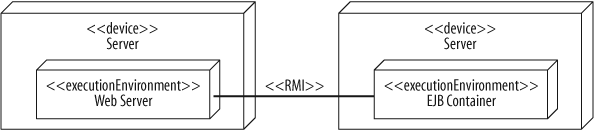
Assigning a stereotype to a communication path can sometimes be tricky. RMI is layered using a TCP/IP transport layer. So, should you assign an <<RMI>> or a <<TCP/IP>> stereotype? As a rule of thumb, your communication stereotype should be as high-level as possible because it communicates more about your system. In this case, <<RMI>> is the right choice; it is higher level, and it tells the reader that you’re using a Java implementation. However, as with all UML modeling, you should tailor the diagram to your audience.
Tip
Communication paths show that the nodes are capable of communicating with each other and are not intended to show individual messages, such as messages in a sequence diagram.
As of UML 2.0, stereotypes are supposed to be specified in a profile, so in theory, you should use only the stereotypes that your profile provides. However, even if you’re not using a profile, your UML tool may allow you to make up any stereotype. Since stereotypes are a good way to show the types of communication in a system, feel free to make your own if necessary and if your tool allows. But if you do, try to keep them consistent. For example, don’t create two stereotypes <<RMI>> and <<Remote Method Invocation>>, which are the same type of communication.
Deployment Specifications
Installing software is rarely as easy as dropping a file on a machine; often you have to specify configuration parameters before your software can execute. A deployment specification is a special artifact specifying how another artifact is deployed to a node. It provides information that allows another artifact to run successfully in its environment.
Deployment specifications are drawn as a rectangle with the stereotype <<deployment spec>>. There are two ways to tie a deployment specification to the deployment it describes:
Draw a dependency arrow from the deployment specification to the artifact, nesting both of these in the target node.
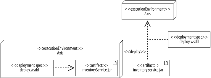
Attach the deployment specification to the deployment arrow, as shown in Figure 15-19.
The deploy.wsdd file, shown in Figure 15-19, is the standard deployment descriptor file that specifies how a web service is deployed to the Axis web service engine. This file states which class executes the web service and which methods on the class can be called. You can list these properties in the deployment specification using the name : type notation. Figure 15-20 shows the deploy.wsdd deployment specification with the properties className and allowedMethods.

The symbol on the right shows an instance of a deployment specification populated with values. Use this notation if you want to show the actual property values instead of just the types.
Tip
This chapter has only briefly mentioned instances of elements in deployment diagrams, but you can model instances of nodes, artifacts, and deployment specifications. In deployment diagrams, many modelers don’t bother to specify that an element is an instance if the intent is clear. However, if you want to specify property values of a deployment specification (as on the right side of Figure 15-20), then this is a rare situation where a UML tool may force you to use the instance notation.
Currently, many UML tools don’t support the deployment specification symbol. If yours is one of them, you can attach a note containing similar information.
You don’t need to list every property in a deployment specification—only properties you consider important to the deployment. For example, deploy.wsdd may contain other properties such as allowed roles, but if you’re not using that property or it’s insignificant (i.e., it’s the same for all your web services), then leave it out.
When to Use a Deployment Diagram
Deployment diagrams are useful at all stages of the design process. When you begin designing a system, you probably know only basic information about the physical layout. For example, if you’re building a web application, you may not have decided which hardware to use and probably don’t know what your software artifacts are called. But you want to communicate important characteristics of your system, such as the following:
Your architecture includes a web server, application server, and database.
Clients can access your application through a browser or through a richer GUI interface.
The web server is protected with a firewall.
Even at this early stage you can use deployment diagrams to model these characteristics. Figure 15-21 shows a rough sketch of your system. The node names don’t have to be precise, and you don’t have to specify the communication protocols.

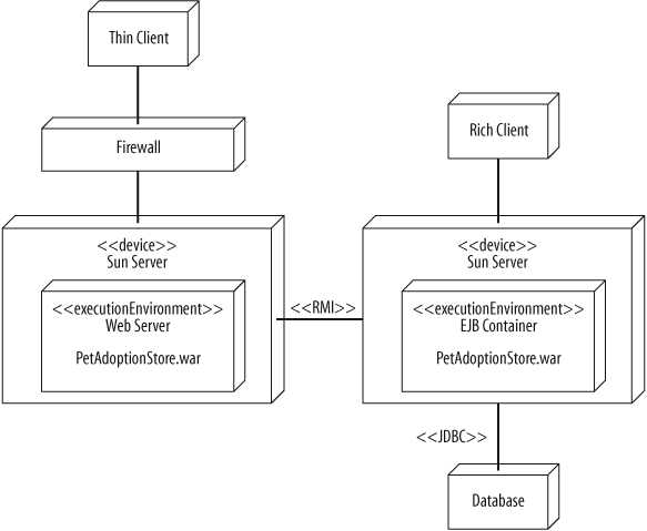
Deployment diagrams are also useful in later stages of software development. Figure 15-22 shows a detailed deployment diagram specifying a J2EE implementation of the system.
Figure 15-22 is more specific about the hardware types, the communication protocols, and the allocation of software artifacts to nodes. A detailed deployment diagram, such as Figure 15-22, could be used be used as a blueprint for how to install your system.
You can revisit your deployment diagrams throughout the design of your system to refine the rough initial sketches, adding detail as you decide which technologies, communication protocols, and software artifacts will be used. These refined deployment diagrams allow you to express the current view of the physical system layout with the system’s stakeholders.
What’s Next?
You’ve finished learning the fundamental UML concepts, but read on to the appendixes for an overview of some advanced modeling techniques. The appendices introduce you to the Object Constraint Language (OCL), which is a rigorous way to show constraints in your diagrams, and Profiles, which allow you to define and use a custom UML vocabulary. It’s helpful to review these appendices to get a feel for extra precision you can add to your model and extra capabilities that result from that precision. The Object Constraint Language is covered in Appendix A; UML profiles are described in Appendix B.