This chapter presents a variety of computational devices which can be employed to solve linear programming problems which depart from the basic structure depicted in Chapter 3 (3.1). In particular, we shall consider “≥” as well as “=” structural constraints, the minimization of the objective, and problems involving unrestricted variables.

5.1 The M‐Penalty Method

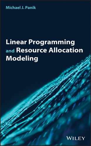
Let us assume that we are faced with solving a linear program whose structural constraint system involves a mixture of structural constraints, e.g. the said problem with its mixed structural constraint system (involving “≤,” “≥,” and “=” structural constraints) might appear as

We noted in Chapter 3 that to convert a “≤” structural constraint to standard form (i.e. to an equality) we must add a nonnegative slack variable to its left‐hand side. A similar process holds for “≥” structural constraints – this time we will subtract a nonnegative surplus variable from its left‐hand side. So for x₃ ≥ 0 a slack variable and x₄ ≥ 0 a surplus variable, the preceding problem, in form, becomes

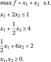
The associated simplex matrix thus appears as

Since this matrix does not contain within it a fourth‐order identity matrix, an initial basic feasible solution does not exist, i.e. we lack a starting point from which to initiate the various rounds of the simplex method because not all of the original structural constraints are of the “≤” variety. So in situations where some or all of the original structural constraints are of the “≥” or “=” form, specific steps must be taken to obtain an identity matrix and thus a starting basic feasible solution.

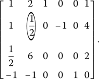
To this end, let us transform the augmented structural constraint system into what is termed the artificial augmented structural constraint systemA_*X_* = b by introducing an appropriate number of nonnegative artificial variables (one for each “≥” and “=” structural constraint), so named because these variables are meaningless in terms of the formulation of the original structural constraint system that contains only legitimate variables. If x₅, x₆ ≥ 0 depict artificial variables (we will always introduce only enough artificial variables to obtain an initial identity matrix), then the A_*X_* = b system appears as

where

and X_a is a vector of artificial variables. Here the vectors within A_* corresponding to artificial variables are termed artificial vectors and appear as a set of unit column vectors. Note that columns 3, 5, and 6 yield a third‐order identity matrix and thus an initial basic feasible solution to A_*X_* = b once the remaining variables are set equal to zero, namely x₃ = 1, x₅ = 4, and x₆ = 2.

While we have obtained an initial basic feasible solution to A_*X_* = b, it is not a feasible solution to the original structural constraint system , the reason being that x₅, x₆ ≠ 0. Hence any basic feasible solution to the latter system must not admit any artificial variable at a positive level. In this regard, if we are to obtain a basic feasible solution to the original linear programming problem, we must utilize the simplex process to remove from the initial basis (i.e. from the identity matrix) all artificial vectors and substitute in their stead an alternative set of vectors chosen from those remaining in A_*. In doing so we ultimately obtain the original structural constraint system itself. Hence all artificial variables are to become nonbasic or zero with the result that a basic feasible solution to emerges wherein the basis vectors are chosen from the coefficient matrix of this system. To summarize: any basic feasible solution to A_*X_* = b which is also a basic feasible solution to has all artificial variables equal to zero.

The computational technique that we shall employ to remove the artificial vectors from the basis is the M‐penalty method (Charnes et al. 1953). Here, extremely large unspecified negative coefficients are assigned to the artificial variables in the objective function in order to preclude the objective function from attaining a maximum as long as any artificial variable remains in the set of basic variables at a positive level. In this regard, for a sufficiently large M > 0, if the coefficient on each artificial variable in the objective function is −M, then the artificial linear programming problem may be framed as:

(5.1)

wherein f is termed the artificial objective function. In terms of the preceding example problem, (5.1) becomes

The simplex matrix associated with this problem is then

(5.2)

To obtain an identity matrix within (5.2), let us multiply both the second and third rows of the same by −M and form their sum as

If this row is then added to the objective function row of (5.2), the new objective function row is

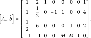
(Note that the first two components of this composite row are each composed of an integer portion and a portion involving M.) To simplify our pivot operations, this transformed objective function row will be written as the sum of two rows. i.e. each objective function term will be separated into two parts, one that does not involve M and one appearing directly beneath it that does. Hence the preceding objective function row now appears as

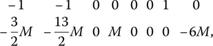
where this double‐row representation actually depicts the single objective function row of the simplex matrix. In view of this convention, (5.2) becomes

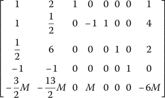
with columns 3, 5, 6, and 7 yielding a fourth‐order identity matrix. Hence, the initial basic feasible solution to the artificial linear program is x₃ = 1, x₅ = 4, x₆ = 2, and f = 6M. And since f is expressed in terms of M, it is evident that the objective function cannot possibly attain a maximum with artificial vectors in the basis.

Before examining some additional example problems dealing with the implementation of this technique, a few summary comments pertaining to the salient features of the M‐penalty method will be advanced. First, once an artificial vector leaves the basis, it never reenters the basis. Alternatively, once an artificial variable turns nonbasic, it remains so throughout the remaining rounds of the simplex process since, if an artificial variable increases in value from zero by a positive amount, a penalty of −M is incurred and f concomitantly decreases. Since the simplex process is one for which f is nondecreasing between succeeding pivot rounds, this possibility is nonexistent. So as the various rounds of the simplex process are executed, we may delete from the simplex matrix those columns corresponding to artificial vectors that have turned nonbasic. Next, if the maximal solution to the artificial problem has all artificial variables equal to zero, then its component is a maximal solution to the original problem with the values of the artificial and original objective functions being the same. Finally, if the maximal solution to the artificial problem contains at least one positive artificial variable, then the original problem possesses no feasible solution (we shall return to this last point later on when a detailed analysis pertaining to the questions on inconsistency and redundancy of the structural constraints is advanced).

5.2 Inconsistency and Redundancy

We now turn to a discussion of the circumstances under which all artificial vectors appearing in the initial basis of the artificial linear programming problem may be removed from the basis in order to proceed to an optimal basic feasible solution to the original problem. In addition, we shall also determine whether the original augmented structural constraint equalities are consistent, and whether any subset of them is redundant. Let us assume that from an initial basic feasible solution to the artificial problem we obtain a basic solution for which the optimality criterion is satisfied. Here one of three mutually exclusive and collectively exhaustive results will hold:

1. The basis contains no artificial vectors.
2. The basis contains one or more artificial vectors at the zero level.
3. The basis contains one or more artificial vectors at a positive level.

Let us discuss the implications of each case in turn.

First, if the basis contains no artificial vectors, then, given that the optimality criterion is satisfied, it is evident that we have actually obtained an optimal basic feasible solution to the original problem. In this instance the original structural constraints are consistent and none is redundant, i.e. if there exists at least one basic feasible solution to the original structural constraint system, the simplex process will remove all artificial vectors from the basis and ultimately reach an optimal solution to the same (a case in point was Example 5.1).

We next turn to the case where the basis contains one or more artificial vectors at the zero level. With all artificial variables equal to zero, we have a feasible solution to , i.e. the original structural constraint equations are consistent. However, there still exists the possibility of redundancy in the original structural constraint system. Upon addressing ourselves to this latter point, we find that two alternative situations merit our consideration. To set the stage for this discussion, let Y_j denote the jth legitimate nonbasic column of the optimal simplex matrix. In this regard, we first assume that y_ij, the ith component of Y_j, is different from zero for one or more j and for one or more i∈ A, where A denotes an index set consisting of all is corresponding to artificial basis vectors e_i. Now, if from some j = j′ we find that it follows that the associated artificial basis vector e_i may be removed from the basis and replaced by . Since the artificial vector currently appears in the basis at the zero level, also enters the basis at the zero level, with the result that the optimal value of the objective function is unchanged in the new basic feasible solution. If this process is repeated until all artificial vectors have been removed from the basis, we obtain a degenerate optimal basic feasible solution to the original problem involving only real or legitimate variables. In this instance none of the original structural constraints within is redundant. Next, if this procedure does not remove all artificial vectors from the basis, we ultimately reach a state where y_ij = 0 for all Y_j and all remaining i∈ A. Under this circumstance we cannot replace any of the remaining artificial vectors by some Y_j and still maintain a basis. If we assume that there are k artificial vectors in the basis at the zero level, every column of the (m × m) matrix may be written as a linear combination of the m−k linearly independent columns of appearing in the basis, i.e. the k artificial vectors are not needed to express any column of in terms of basis vectors. Hence so that only m−k rows of are linearly independent, thus implying that k of the original structural constraints are redundant. (As a practical matter, since inequality structural constraints can never be redundant – each is converted into an equality by the introduction of its “own” slack or surplus variable – our search for redundant structural constraints must be limited to only some subset of equations appearing in , namely those expressed initially as strict equalities.) To identify the specific structural constraints within that are redundant, we note briefly that if the artificial basis vector e_h remains in the basis at the zero level and y_hk = 0 for all legitimate nonbasis vectors Y_j, then the hth structural constraint of is redundant. In this regard, if at some stage of the simplex process we find that the artificial vector e_h appears in the basis at the zero level, with y_hj = 0 for all Y_j, then, before executing the next round of the simplex routine, we may delete the hth row of the simplex matrix containing the zero‐valued artificial variable along with the associated artificial basis vector e_h. The implication here is that any redundant constraint may be omitted from the original structural constraint system without losing any information contained within the latter.

We finally encounter the case where one or more artificial vectors appear in the basis at a positive level. In this instance, the basic solution generated is not meaningful, i.e. the original problem possesses no feasible solution since otherwise the artificial vectors would all enter the basis at a zero level. Here the original system either has no solution (the structural constraints are inconsistent) or has solutions that are not feasible. To distinguish between these two alternatives, we shall assume that the optimality criterion is satisfied and y_ij ≤ 0 for legitimate nonbasis vectors Y_j and for those i∈ A. If for some j = j′ we find that we can insert into the basis and remove the associated artificial basis vector e_i and still maintain a basis. However, with the new basic solution will not be feasible since enters the basis at a negative level. If this process is repeated until all artificial vectors have been driven from the basis, we obtain a basic though nonfeasible solution to the original problem involving only legitimate variables (see Example 5.3). Next, if this procedure does not remove all artificial vectors from the basis, we ultimately obtain a state where y_ij = 0 for all Y_j and for all i remaining in A. Assuming that there are k artificial vectors in the basis, every column of may be written as a linear combination of the m − k legitimate basis vector so that But the fact that k artificial columns from appear in the basis at positive levels implies that b is expressible as a linear combination of more than m − k basis vectors so that In this regard, the original structural constraint system is inconsistent and thus does not possess a solution (see Example 5.4).

A consolidation of the results obtained in this section now follows. Given that the optimality criterion is satisfied: (i) if no artificial vectors appear in the basis, then the solution is an optimal basic feasible solution to the original linear programming problem. In this instance, the original structural constraints are consistent and none is redundant; (ii) if a least one artificial vector appears in the basis at a zero level, then is consistent and we either obtain a degenerate optimal basic feasible solution to the original problem or at least one of the original structural constraints is redundant; and (iii) if at least one artificial vector appears in the basis at a positive level, the original problem has no feasible solution since either represents an inconsistent system or there are solutions but none is feasible.

5.3 Minimization of the Objective Function

Let us assume that we desire to

As we shall now see, to solve this minimization problem, simply transform it to a maximization problem, i.e. we shall employ the relationship min f =  − max {−f }. To this end, we state Theorem 5.1:

5.4 Unrestricted Variables

Another variation of the basic linear programming problem is that (one or more of) the components of X may be unrestricted in sign, i.e. may be positive, negative, or zero. In this instance, we seek to

To handle situations of this sort, let the variable x_k be expressed as the difference between two nonnegative variables as

(5.4)

So by virtue of this transformation, the above problem may be rewritten, for X = X′ − X″, as

Then the standard simplex technique is applicable since all variables are now nonnegative. Upon examining the various subcases that emerge, namely:

1. if then x_k > 0;
2. if then x_k < 0; and
3. if then x_k = 0.

we see that x_k, depending on the relative magnitude of and , is truly unrestricted in sign.

One important observation relative to using (5.4) to handle unrestricted variables is that any basic feasible solution in nonnegative variables cannot have both and in the set of basic variables since, for the kth column of so that and are not linearly independent and thus cannot both constitute columns of the basis matrix.

5.5 The Two‐Phase Method

In this section, we shall develop an alternative procedure for solving a linear programming problem involving artificial variables. The approach will be to frame the simplex method in terms of two successive phases, Phase I (PI) and Phase II (PII) (Dantzig et al. 1955). In PI, we seek to drive all artificial variables to zero by maximizing a surrogate objective function involving only artificial variables. If the optimal basis for the PI problem contains no artificial vectors, or contains one or more artificial vectors at the zero level, then PII is initiated. However, if the optimal PI basis contains at least one artificial vector at a positive level, the process is terminated. If PII is warranted, we proceed by maximizing the original objective function using the optimal PI basis as a starting point, i.e. the optimal PI basis provides an initial though possibly nonbasic feasible solution to the original linear program.

PHASE I. For the PI objective function, the legitimate variables will be assigned zero coefficients while each artificial variable is given a coefficient of −1. Then the PI surrogate linear programming problem may be formulated as: maximize the infeasibility form

(5.5)

Note that with X_a ≥ O, it must be the case that max{g} ≤ 0. Additionally, the largest possible value that g can assume is zero, and this occurs only if the optimal PI basis contains no artificial vectors, or if any artificial vectors remaining in the said basis do so at the zero level. So if max{g} < 0, at least one artificial vector remains in the optimal PI basis at a positive level.

Looking to some of the salient features of the PI routine: (i) as with the M‐penalty method, an artificial vector never reenters the basis once it has been removed (here too the columns of the simplex matrix corresponding to artificial vectors that have turned nonbasis may be deleted as pivoting progresses); (ii) during PI, the sequence of vectors that enters and leaves the basis is the same as in the M‐penalty method; and (iii) if g becomes zero before the optimality criterion is satisfied, we may terminate PI and proceed directly to PII.

Once the PI optimality criterion is satisfied, the optimal basis will exhibit one of three mutually exclusive and collectively exhaustive characteristics:

1. max{g} = 0 and no artificial vectors remain in the basis;
2. max{g} = 0 and one or more artificial vectors remain in the basis at the zero level; and
3. max{g} < 0 and one or more artificial vectors remain in the basis at a positive level.

If case one obtains, the optimal PI basis provides a basic feasible solution to the original (primal) problem; the original structural constraints are consistent and none is redundant. For case two, we obtain a feasible solution to the original problem; the original structural constraints are consistent, though possibly redundant. And for case three, the surrogate problem has no feasible solution with X_a = O and thus the original problem has no feasible solution as well. So, if either case one or case two emerges at the end of PI, there exists at least one feasible solution to the original problem. In this regard, we advance to PII.

PHASE II. Since we ultimately want to maximize f(X), the optimal PI simplex matrix is transformed into the initial PII simplex matrix by respecifying the objective function coefficients. That is, during PII, the coefficients on the legitimate variables are the same as those appearing in the original objective function while the coefficients on the artificial variables are zero; the PII objective function is the original objective function f(X) itself. Hence, the sequence of operations underlying the phase‐two method may be expressed as:

(5.6)

We now examine the implications for PII of the aforementioned characteristics of the optimal PI simplex matrix. For case one above, the optimal PI basis provides an initial basic feasible solution to the original problem. Once the PII objective function is introduced, pivoting proceeds until an optimal basic feasible solution to the original linear program is attained. Turning to case two, while we have obtained a feasible nonbasic solution to the original problem, there still remains the question of redundancy in the original structural constraints AX = b. Also, we need to develop a safeguard against the possibility that one or more artificial vectors currently in the initial PII basis at the zero level will appear in some future basis at a positive level as the PII pivot operations are executed.

Our discussion of redundancy here is similar to that advanced for the M‐penalty method. Let us assume that within the optimal PI simplex matrix y_ij = 0 for all legitimate nonbasis vectors and for all i ∈ A. In this instance, none of the artificial basis vectors e_i can be replaced by the so that there is redundancy in the original structural constraint equalities. In this regard, if there are k artificial vectors in the basis at the zero level, then, at the end of PI, we may simply delete the k rows of the simplex matrix containing the zero‐valued artificial variables along with the associated artificial basis vectors e_i. Then PII begins with a basis of reduced size and pivoting is carried out until an optimal basic feasible solution to the original problem is attained.

We next examine a procedure that serves to guard against the possibility that an artificial vector appearing in the initial PII basis at the zero level manifests itself in some future basis at a positive level. Let us assume that for some j = j′ the vector is to enter the basis and with for at least one i ∈ A. In this circumstance, the artificial vectors for which will not be considered as candidates for removal from the basis. Rather, some legitimate vector will be removed with the result that the artificial basis vectors for which appear in the new basis at a positive level. To avoid this difficulty, instead of removing a legitimate vector from the basis, let us adopt the policy of arbitrarily removing any one of the artificial basis vectors e_i with . The result will be a feasible solution to the original problem wherein enters the new basis at the zero level (since the artificial vector that it replaced was formerly at the zero level). With the value of the incoming variable equal to zero, the values of the other basic variables for the new solution are the same as in the preceding solution. Hence the value of the objective function for the new solution must be the same as the previous one (see Example 5.8).