13
Simplex‐Based Methods of Optimization
13.1 Introduction
In this chapter the standard simplex method, or a slight modification thereof, will be used to solve an assortment of specialized linear as well as essentially or structurally nonlinear decision problems. In this latter instance, a set of transformations and/or optimality conditions will be introduced that linearizes the problem so that the simplex method is only indirectly applicable. An example of the first type of problem is game theory, while the second set of problems includes quadratic and fractional functional programming.
13.2 Quadratic Programming
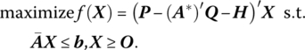
The quadratic programming problem under consideration has the general form

Here, the objective function is the sum of a linear form and a quadratic form and is to be optimized in the presence of a set of linear inequalities. Additionally, both C and X are of order (p × 1), Q is a (p × p) symmetric coefficient matrix, A is the (m × p) coefficient matrix of the linear structural constraint system, and b (assumed ≥O) is the (m × 1) requirements vector. If Q is not symmetric, then it can be transformed, by a suitable redefinition of coefficients, into a symmetric matrix without changing the value of X′QX. For instance, if a matrix A from X′AX is not symmetric, then it can be replaced by a symmetric matrix B if ![]() for all i, j or B = (A + A′)/2. Thus, bij + bji = 2bij = aij + aji is the coefficient of xixj, i ≠ j, in
for all i, j or B = (A + A′)/2. Thus, bij + bji = 2bij = aij + aji is the coefficient of xixj, i ≠ j, in

So if
then, under this transformation,

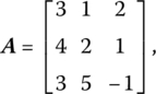
In this regard, for the quadratic function ![]() the coefficient matrix may simply be assumed symmetric and written
the coefficient matrix may simply be assumed symmetric and written

or if
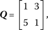
the associated quadratic function may be expressed as ![]() For additional details on quadratic forms, see Appendix 13.A.
For additional details on quadratic forms, see Appendix 13.A.
We mentioned in earlier chapters that an optimal solution to a linear programming problem always occurs at a vertex (extreme point) of the feasible region K = {X|AX ≤ b, X ≥ O} or at a convex combination of a finite number of extreme points of K (i.e. along an edge of K). This is not the case for a quadratic programming problem. An optimal solution to a quadratic program may occur at an extreme point or along an edge or at an interior point of K (see Figure 13.1a–c, respectively, wherein K and the contours of f are presented).
Figure 13.1 (a) Constrained maximum of f at extreme point A. (b) Constrained maximum of f occurs along the edge BC. (c) Constraints not binding at A.
To further characterize the attainment of an optimal solution to (13.1), let us note that with K a convex set, any local maximum of f will also be the global maximum if f is concave. Clearly C′X is concave since it is linear, while X′QX is concave if it is negative semi‐definite or negative definite. Thus, f = C′X + X′QX is concave (since the sum of a finite number of concave functions is itself a concave function) on K so that the global maximum of f is attained. In what follows, we shall restrict Q to the negative definite case. Then f may be characterized as strictly concave so that it takes on a unique or strong global maximum on K.1 If X′QX is negative semi‐definite, then it may be transformed to a negative definite quadratic form by making an infinitesimally small change in the diagonal elements of Q, i.e. X′QX is replaced by X′(Q − εIp)X = X′QX − εX′IpX < 0 since X′QX ≤ 0 for any X and −εX′IpX < 0 for any X ≠ O.
From (13.1) we may form the Lagrangian function
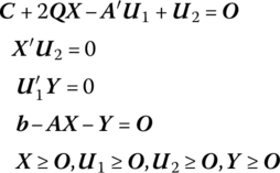
Then from the Karush‐Kuhn‐Tucker necessary and sufficient conditions for a constrained maximum (12.4),
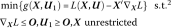
Before proceeding to the development of a solution algorithm for the quadratic programming problem, let us examine an important interpretation of (13.2). Specifically, if Xo solves (13.1), then there exists a vector ![]() such that (Xo,
such that (Xo,![]() ) is a saddle point (see Chapter 12 for a review of this concept) of the Lagrangian
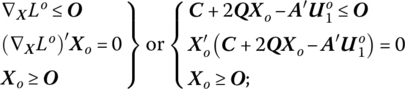
) is a saddle point (see Chapter 12 for a review of this concept) of the Lagrangian ![]() in which case (13.2) holds. To see this, we need only note that if L(X, U1) has a local maximum in the X direction at Xo, then it follows from (13.2a, b, e) that
in which case (13.2) holds. To see this, we need only note that if L(X, U1) has a local maximum in the X direction at Xo, then it follows from (13.2a, b, e) that
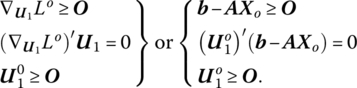
while if L(Xo, U1) attains a minimum in the U1 direction at ![]() , then, from (13.2d, c, e),
, then, from (13.2d, c, e),
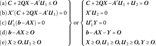
Upon examining (13.2) we see that solving the quadratic programming problem amounts to finding a solution in 2(m + p) nonnegative variables to the linear system
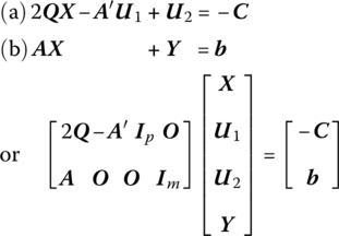
that satisfies the m + p (nonlinear) complementary slackness conditions ![]() Under this latter set of restrictions, at least p of the 2p xjs, u2js must be zero while at least m of the 2m u1is, yis must equal zero. Thus, at least m + p of the 2(m + p) variables xj, u2j, u1j, yi must vanish at the optimal solution. In this regard, an optimal solution to (13.2.1) must be a basic feasible solution (Barankin and Dorfman 1958). So, if the (partitioned) vector
Under this latter set of restrictions, at least p of the 2p xjs, u2js must be zero while at least m of the 2m u1is, yis must equal zero. Thus, at least m + p of the 2(m + p) variables xj, u2j, u1j, yi must vanish at the optimal solution. In this regard, an optimal solution to (13.2.1) must be a basic feasible solution (Barankin and Dorfman 1958). So, if the (partitioned) vector ![]() is a feasible solution to (13.2.1) and the complementary slackness conditions are satisfied (no more than m + p of the mutually complementary variables are positive), then the resulting solution is also a basic feasible solution to (13.2.1) with the Xo component solving the quadratic programming problem.
is a feasible solution to (13.2.1) and the complementary slackness conditions are satisfied (no more than m + p of the mutually complementary variables are positive), then the resulting solution is also a basic feasible solution to (13.2.1) with the Xo component solving the quadratic programming problem.
To actually obtain an optimal basic feasible solution to (13.2.1) we shall use the complementary pivot method presented in Section 13.4. But first we look to dual quadratic programs.
13.3 Dual Quadratic Programs
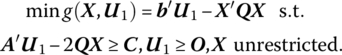
A well‐known result from duality theory in generalized nonlinear programming that is applicable for our purposes here is that if the Lagrangian for the primal quadratic program (13.1) is written as ![]() then the dual quadratic program appears as
then the dual quadratic program appears as
or
In what follows, a few important theorems for quadratic programming problems will be presented. The first two demonstrate the similarity between linear and quadratic programming as far as the relationship of the primal and dual objective functions is concerned. To this end, we state Theorems 13.1 as follows.
Next,
Finally, the principal duality result of this section is presented by
13.4 Complementary Pivot Method
(Lemke 1965)
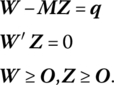
A computational routine that explicitly requires that a complementarity condition holds at each iteration is Lemke’s complementary pivot method. This technique is designed to generate a solution to the linear complementarity problem (LCP): given a vector q ∈ ℛn and an nth order matrix M, find a vector Z ∈ ℛn such that

If W = q + MZ, then (13.7) becomes: find vectors W, Z ∈ ℛn, such that
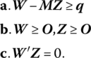
Here ![]() is called the complementarity condition, where the variables wi and zi, called a complementary pair, are said to be complements of each other, i.e. at least one variable in each pair (wi, zi,) must be zero.
is called the complementarity condition, where the variables wi and zi, called a complementary pair, are said to be complements of each other, i.e. at least one variable in each pair (wi, zi,) must be zero.
A nonnegative solution (W, Z) to the linear system (13.8a) is called a feasible solution to the LCP. Moreover, a feasible solution (W, Z) to the LCP that also satisfies the complementarity condition on W′ Z = 0 is termed a complementary solution. (Note that (13.7) and (13.8) contain no objective function; and there is only a single structural constraint in the variables W, Z, namely the complementary restriction W′ Z = 0.)
If q ≥ O, then there exists a trivial complementary basic solution given by W = q, Z = O. Hence (13.8) has a nontrivial solution only when q ≱ O. In this circumstance, the initial basic solution given by W = q, Z = O is infeasible even if the complementarity condition W′ Z = 0 holds.
For the general quadratic program
let us repeat the Karush‐Kuhn‐Tucker conditions for (13.1) as
or

Let us define

Then (13.9) can be rewritten in condensed form as
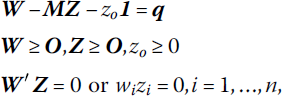
As we shall now see, these conditions are solved by a pivoting process. This will be accomplished by introducing an auxiliary (artificial) variable zo ∈ ℛ and a sum vector 1 ∈ ℛn + m into (13.10) so as to obtain
for at least n−1 of the i values given zo ≥ 0.
The algorithm starts with an initial basic feasible solution to (13.8) of the form W = q, Z ≥ O, where q ≱ O. To avoid having at least one wi < 0, the nonnegative artificial variable zo will be introduced at a sufficiently positive level (take ![]() ) into the left‐hand side of W − MZ = q. Hence our objective is to find vectors W, Z and a variable zo such that (13.11) holds.
) into the left‐hand side of W − MZ = q. Hence our objective is to find vectors W, Z and a variable zo such that (13.11) holds.
With each new right‐hand side value qi + zo nonnegative in (13.11), a basic solution to the same amounts to W + zo1 ≥ O, Z = O. While this basic solution is nonnegative and satisfies all the relationships in (13.11) (including complementarity), it is infeasible for the original LCP (13.8) since zo > 0. A solution such as this will be termed an almost complementary basic solution. So while a complementary basic solution to (13.8) is one that contains exactly one basic variable from each complementary pair of variables (wi, zi), i = 1, …, n, an almost complementary basic solution of (13.8) is a basic solution for (13.11) in which zo is a basic variable and there is exactly one basic variable from each of only n − 1 complementary pairs of variables.
The complementary pivot method has us move from one almost complementary basic solution of (13.8) to another until we reach a complementary basic solution to (13.8), in which case we have wi, zi = 0 for all i = 1, …, n. At this point, the algorithm is terminated. To see this, let us rewrite (13.11) as

with associated simplex matrix
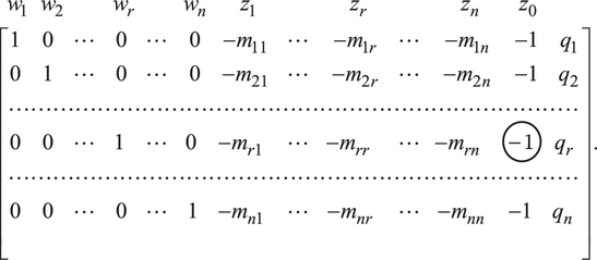
To find an initial almost complementary basic solution, the artificial variable zo is made basic by having it replace the current basic variable with the most negative qi value. Suppose ![]() Hence, zo replaces wr in the set of basic variables. To accomplish this we pivot on the (circled) element −1 in (13.12). This yields
Hence, zo replaces wr in the set of basic variables. To accomplish this we pivot on the (circled) element −1 in (13.12). This yields
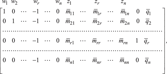
where

As (13.13) reveals, an almost complementary basic solution to (13.8) is ![]()
The complementary pivot algorithm generates a sequence of almost complementary basic solutions until zo becomes nonbasic or zero. Moreover, pivoting must be done in a fashion such that: (i) complementarity between the variables wi, zi is maintained at each iteration; and (ii) each successive basic solution is nonnegative.
Now, at the moment, both wr and zr are nonbasic (wrzr = 0 is satisfied). Since wr turned nonbasic in (13.13), the appropriate variable to choose for entry into the set of basic variables is its complement zr. In fact, this selection criterion for determining the nonbasic variable to become basic is referred to as the complementary pivot rule: choose as the incoming basic variable the one complementary to the basic variable, which just turned nonbasic.
Once the entering variable is selected, the outgoing variable can readily be determined from the standard simplex exit criterion, i.e. wk is replaced by zk in the set of basic variables if

A pivot operation is then performed using ![]() as the pivot element. Once wk turns nonbasic, the complementary pivot rule next selects zk for entry into the set of basic variables. Complementary pivoting continues until one of two possible outcomes obtains, at which point the complementary pivot algorithm terminates:
as the pivot element. Once wk turns nonbasic, the complementary pivot rule next selects zk for entry into the set of basic variables. Complementary pivoting continues until one of two possible outcomes obtains, at which point the complementary pivot algorithm terminates:
- The simplex exit criterion selects row r as the pivot row and zo turns nonbasic. The resulting solution is a complementary basic solution to (13.8).
- No
 in (13.14). (In this latter instance, the problem either has no feasible solution or, if a primal (dual) feasible solution exists, the primal (dual) objective function is unbounded.)
13.5 Quadratic Programming and Activity Analysis
In Chapter 7 we considered a generalized linear activity analysis model in which a perfectly competitive firm produces p different products, each corresponding to a separate activity operated at the level xj, j = 1, …, p. The exact profit maximization model under consideration was given by (7.27), i.e.

or, in matrix form,

In this formulation, total revenue is ![]() total variable input cost is
total variable input cost is ![]() and total conversion cost is
and total conversion cost is ![]() Here pj (the jth component of P) is the constant price per unit of output of activity j, qi (the ith component of Q) is the constant unit price of the ith variable input, and
Here pj (the jth component of P) is the constant price per unit of output of activity j, qi (the ith component of Q) is the constant unit price of the ith variable input, and ![]() is the cost of converting the m − l fixed inputs to the operation of the jth activity at the unit level, where rij (the ith component of rj) is the cost of converting one unit of ith fixed factor to the jth activity.
is the cost of converting the m − l fixed inputs to the operation of the jth activity at the unit level, where rij (the ith component of rj) is the cost of converting one unit of ith fixed factor to the jth activity.
Let us now relax the assumption of given product prices pj and assume, instead, that the firm is a monopolist in the markets for the p outputs. In this regard, there exists a downward sloping demand curve for each of the p products so that an inverse relationship exists between pj and xj, e. g., pj = aj − bjxj, dpj/dxj = − bj < 0. Then total revenue from sales of the output of the jth activity ![]() Hence total revenue is now
Hence total revenue is now ![]() where a′ = (a1, …, ap) and B is a (p × p) symmetric positive definite diagonal matrix of the form
where a′ = (a1, …, ap) and B is a (p × p) symmetric positive definite diagonal matrix of the form

Clearly total revenue under this new specification of price behavior is the sum of a linear and a quadratic form in X. Moreover, the derivative of total revenue TR with respect to X is marginal revenue MR or

i.e. the jth component of this vector is the marginal revenue from the sale of xj or MRj = dTRj/dxj = aj − 2bjxj, j = 1, …, p.
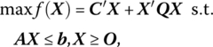
In view of this respecification of total revenue, the above profit maximization model appears as

or

Additionally, the Karush‐Kuhn‐Tucker necessary and sufficient conditions for an optimum appear (using (13.2)) as:
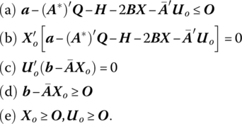
Upon examining (13.20) we see that ![]() or, in terms of the individual components of this inequality, the imputed cost of operating activity j at the unit level is at least as great as the gross profit margin for activity j, the latter being expressed as the marginal revenue of activity j less the total cost of operating activity j at the unit level less the cost of converting the m − l fixed factors to the operation of the jth activity at the unit level. (The interpretation of (13.20b, c, d, e) is similar to the one advanced for (12.28) and will not be duplicated here.)
or, in terms of the individual components of this inequality, the imputed cost of operating activity j at the unit level is at least as great as the gross profit margin for activity j, the latter being expressed as the marginal revenue of activity j less the total cost of operating activity j at the unit level less the cost of converting the m − l fixed factors to the operation of the jth activity at the unit level. (The interpretation of (13.20b, c, d, e) is similar to the one advanced for (12.28) and will not be duplicated here.)
Turning next to the dual program associated with (13.19) we have

or, for X fixed at Xo (the optimal solution vector to the primal quadratic program),

Either (13.21) or (13.21.1) is appropriate for considering the dual program from a computational viewpoint. However, for purposes of interpreting the dual program in an activity analysis context, let us first examine the generalized nonlinear dual objective from which g (X, U) in (13.21) was derived, namely

The first term on the right‐hand side of (13.22) is simply the total imputed value of the firm’s supply of fixed or scarce resources (the dual objective in a linear activity analysis model). The second term can be interpreted as economic rent (the difference between total profit and the total imputed cost of all inputs used).3 Finally, if the square‐bracketed portion of the third term (which is nonpositive by virtue of (13.20a)) is thought of as a set of accounting or opportunity losses generated by a marginal increase in the level of operation of activity j, then the entire third term is a weighted sum of these losses (the weights being the various activity levels) and thus amounts to the marginal opportunity loss of all outputs. At an optimal solution, however, (13.20b) reveals that this third term is zero (Balinski and Baumol 1968). Next, upon examining the dual structural constraint in (13.21) we see that ![]() so that, as in the linear activity model, the imputed cost of operating each activity at the unit level must equal or exceed its gross profit margin. In sum, the dual problem seeks a constrained minimum to the total imputed value of all scarce resources plus payments to economic rent plus losses due to unprofitable activities.
so that, as in the linear activity model, the imputed cost of operating each activity at the unit level must equal or exceed its gross profit margin. In sum, the dual problem seeks a constrained minimum to the total imputed value of all scarce resources plus payments to economic rent plus losses due to unprofitable activities.
13.6 Linear Fractional Functional Programming
(Charnes and Cooper 1962; Lasdon 1970; Martos 1964; Craven 1978)
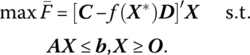
In what follows we shall employ the simplex algorithm to solve an optimization problem, known as a linear fractional programming problem, in which the objective function is nonlinear in that it is expressed as the ratio of two linear functions and the variables must satisfy a system of linear inequalities and nonnegativity conditions. Specifically, let us
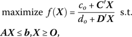
where co, do are scalars, C and D are (p × 1) vectors with components cj, dj respectively, j = 1, …, p, and A is of order (m × p). Although f is neither convex nor concave, its contours (co + C′X)/(do + D′X) = constant are hyperplanes. Moreover, any finite constrained local maximum of f is also global in character and occurs at an extreme point of the feasible region K. That is,
Let us next examine a couple of direct (in the sense that no variable transformation or additional structural constraints or variables are introduced) approaches to solving the above fractional program, which mirror the standard simplex method. For the first technique (Swarup 1965), let us start from an initial basic feasible solution and, under the assumption that do + D′X > 0 for all X ε K, demonstrate the conditions under which the objective value can be improved. Doing so will ultimately provide us with a set of conditions that an optimal basic feasible solution must satisfy.
Upon introducing the slack variables xp + 1, …, xn into the structural constraint system, we may write the (m × n) coefficient matrix of the same as A = ![]() , where the (m × m) matrix B = [b1, …, bm] has as its columns the columns of A corresponding to basic variables and the (m × n− m) matrix R contains all remaining columns of A. Then solving for the basic variables in terms of the nonbasic variables we have the familiar equality XB = B−1b − B−1RXR, where
, where the (m × m) matrix B = [b1, …, bm] has as its columns the columns of A corresponding to basic variables and the (m × n− m) matrix R contains all remaining columns of A. Then solving for the basic variables in terms of the nonbasic variables we have the familiar equality XB = B−1b − B−1RXR, where ![]() For XR = O, we have the basic solution XB = B−1b. If XB ≥ O, the solution is deemed feasible. Let us partition the vectors C, D as
For XR = O, we have the basic solution XB = B−1b. If XB ≥ O, the solution is deemed feasible. Let us partition the vectors C, D as
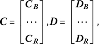
respectively, where the (m × 1) vectors CB, DB contain as their elements the objective function coefficients corresponding to the basic variables while the components of the (n − m × 1) vectors CR, DR correspond to the objective function coefficients associated with nonbasic variables.
Let

and, for those nonbasic columns rj, j = 1, …, n − m, of R, let rj = BYj so that Yj = B−1rj, i.e. Yj is the jth column of B−1R. If ![]() then the optimality evaluators may be expressed as
then the optimality evaluators may be expressed as
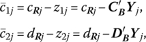
where cRj, dRj are, respectively, the jth component of CR, DR, j = 1, …, n − m.
Our goal is now to find an alternative basic feasible solution that exhibits an improved value of f = zB1/zB2. If we change the basis one vector at a time by replacing bj by rj, we obtain a new basis matrix ![]() where
where ![]() Then the values of the new basic variables are, from (4.11.1),
Then the values of the new basic variables are, from (4.11.1),
And from (4.12), the new value of the objective function is
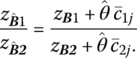
Clearly the value of f will improve if
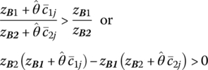
since ![]() given that do + D′X > 0. Simplifying the preceding inequality yields
given that do + D′X > 0. Simplifying the preceding inequality yields
(If ![]() the value of f is unchanged and the degenerate case emerges.)
the value of f is unchanged and the degenerate case emerges.)
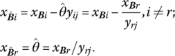
If for any rj we find that Δj > 0 and if at least one component yij of Yj is positive (here Yj corresponds to the first m elements of the jth nonbasic column of the simplex matrix), then it is possible to obtain a new basic feasible solution from the old one by replacing one of the columns of B by rj with the result that ![]() For the entry criterion, let us adopt the convention that the incoming basic variable is chosen according to
For the entry criterion, let us adopt the convention that the incoming basic variable is chosen according to
i.e. xBr enters the set of basic variables. (Note that this choice criterion gives us the largest increase in f.) In addition, the exit criterion is the same as the one utilized by the standard simplex routine. This procedure may be repeated until, in the absence of degeneracy, the process converges to an optimal basic feasible solution. Termination occurs when Δj ≤ 0 for all nonbasic columns rj, j = 1, …, n − m. It is imperative to note that this method cannot be used if both co, do are zero, i.e. if we start from an initial basic feasible solution with CB = CD = O and co = do = 0, then zB1 = zB2 = 0 also and thus Δj = 0 for all j, thus indicating that the initial basic feasible solution is optimal. Clearly, this violates the requirement that do + D′X > 0.
Relative to the second direct technique (Bitran and Novaes 1973) for solving the fractional functional program, let us again assume that do + D′X > 0 for all X ε K and use the standard simplex method to solve a related problem that is constructed from the former and appears as

Here λ equals C minus the vector projection of C onto D (this latter notion is defined as a vector in the direction of D obtained by projecting C perpendicularly onto D). Upon solving (13.29), we obtain the suboptimal solution point X*.
The next step in the algorithm involves utilizing X* to construct a new objective function to be optimized subject to the same constraints, i.e. we now
The starting point for solving (13.30) is the optimal simplex matrix for problem (13.42); all that needs to be done to initiate (13.30) is to replace the objective function row of the optimal simplex matrix associated with (13.29) by the objective in (13.30). The resulting basic feasible solution will be denoted as X**.
If X** = X*, then X* represents the global maximal solution to the original fractional program; otherwise return to (13.30) with X* = X** and repeat the process until the solution vector remains unchanged. (For a discussion on the geometry underlying this technique, see Bitran and Novaes 1973, pp. 25–26.)
13.7 Duality in Linear Fractional Functional Programming
(Craven and Mond 1973, 1976; Schnaible 1976; Wagner and Yuan 1968; Chadha 1971; Kydland 1962; and Kornbluth and Salkin 1972)
To obtain the dual of a linear fractional functional program, let us dualize its equivalent linear program. That is, under the variable transformation Y = tX, t = (do + D′X)−1, the linear fractional programming problem (13.23) or

is equivalent to the linear program
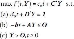
if do + D′X > 0 for all X ε K and for each vector Y ≥ O, the point (t, Y) = (0, Y) is not feasible, i.e. every feasible point (t, Y) has t > 0 (Charnes and Cooper 1962). (This latter restriction holds if K is bounded. For if ![]() is a feasible solution to the equivalent linear program (13.32), then, under the above variable transformation,
is a feasible solution to the equivalent linear program (13.32), then, under the above variable transformation, ![]() If X ε K, then
If X ε K, then ![]() K, θ ≥ 0, thus contradicting the boundedness of K.) In this regard, if
K, θ ≥ 0, thus contradicting the boundedness of K.) In this regard, if ![]() represents an optimal solution to the equivalent linear program, then
represents an optimal solution to the equivalent linear program, then ![]() is an optimal solution to the original fractional problem.
is an optimal solution to the original fractional problem.
To demonstrate this equivalence let
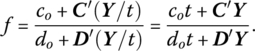
Moreover, AX = A(Y/t) ≤ b or AY − tb ≤ O. If dot + D′Y = 1, then (13.32) immediately follows.
It now remains to dualize (13.32). Let
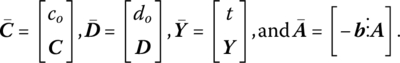
Then (13.32) may be rewritten as

Upon replacing ![]() the preceding problem becomes
the preceding problem becomes

The symmetric dual to this problem is then
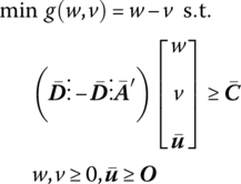
or, for λ = w − v,

As was the case with the primal and dual problems under linear programming, we may offer a set of duality theorems (Theorems 13.5 and 13.6) that indicate the relationship between (13.23), (13.33). To this end, we have
We next have
While (13.33) represents the dual of the equivalent linear program (13.32), what does the general nonlinear dual (Panik 1976) to (13.23) look like? Moreover, what is the connection between the dual variables in (13.33) and those found in the general nonlinear dual to (13.23)? To answer these questions, let us write the said dual to (13.33) as
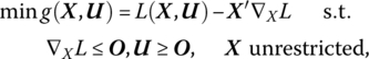
where L(X, U) = (co + C′X)/(do + D′X) + U′(b − AX) is the Lagrangian associated with the primal problem (13.23). In this regard, this dual becomes
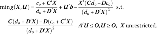
Since t = (do + D′X)−1, the structural constraint in (13.37) becomes
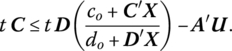
Since at an optimal solution to the primal‐dual pair of problems we must have λ = (co + C′X)/(do + D′X) (see Theorem 13.6), (13.37.1) becomes
Then the structural constraint in (13.37) is equivalent to (13.33b) if ![]() Moreover, when
Moreover, when ![]() the objective in (13.37) simplifies to λ, the same objective as found in (13.33). To summarize, solving (13.32) gives us m + 1 dual variables, one corresponding to each structural constraint. The dual variable for (13.32a) (namely λ) has the value attained by
the objective in (13.37) simplifies to λ, the same objective as found in (13.33). To summarize, solving (13.32) gives us m + 1 dual variables, one corresponding to each structural constraint. The dual variable for (13.32a) (namely λ) has the value attained by ![]() at its optimum. The dual variables for (13.23) are then found by multiplying the dual variables for the constraints (13.32b) by t.
at its optimum. The dual variables for (13.23) are then found by multiplying the dual variables for the constraints (13.32b) by t.
13.8 Resource Allocation with a Fractional Objective
We previously specified a generalized multiactivity profit‐maximization model (7.27.1) as
An assumption that is implicit in the formulation of this model is that all activities can be operated at the same rate per unit of time. However, some activities may be operated at a slower pace than others so that the time needed to produce a unit of output by one activity may vary substantially between activities. Since production time greatly influences the optimum activity mix, the model should explicitly reflect the importance of this attribute. Let us assume, therefore, that activity j is operated at an average rate of tj units per minute (hour, etc.). Then total production time is ![]() where
where ![]() is of order (p × 1). Note that dT/dtj < 0 for each j, i.e. total production time is inversely related to the speed of operation of each activity.
is of order (p × 1). Note that dT/dtj < 0 for each j, i.e. total production time is inversely related to the speed of operation of each activity.
If C denotes the (constant) rate per unit of time of operating the production facility and K represents fixed overhead cost, then the total overhead cost of operating the facility is h(X) = CT′X + K. In view of this discussion, total profit is ![]() We cannot directly maximize this function subject to the above constraints since two different activity mixes do not necessarily yield the same production time so that we must divide
We cannot directly maximize this function subject to the above constraints since two different activity mixes do not necessarily yield the same production time so that we must divide ![]() to get average profit per unit of time
to get average profit per unit of time
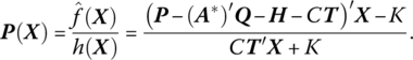
Hence, the adjusted multiactivity profit‐maximization model involves maximizing (13.52) subject to ![]()
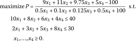
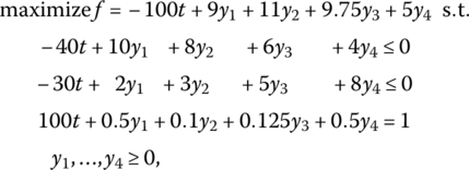
For instance, from Example 7.3 the problem
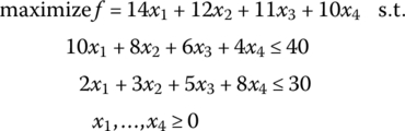
has as its optimal basic feasible solution x1 = 10/19, x3 = 110/19, and f = 1350/19. Moreover, the shadow prices are u1 = 24/19, u2 = 13/19 while the accounting loss figure for products x2, x4 are, respectively, us2 = 3/19, us4 = 10/19. If we now explicitly introduce the assumption that some activities are operated at a faster rate than others, say t1 = 2, t2 = 10, t3 = 8, and t4 = 2, then the preceding problem becomes, for C = 10, K = 100,
Upon converting this problem to the form provided by (13.32), i.e. to
and solving (via the two‐phase method) yields the optimal simplex matrix (with the artificial column deleted)
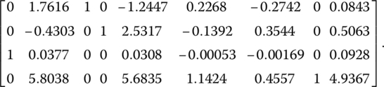
Thus ![]() With Xo = Yo/to, the optimal solution, in terms of the original variables, is
With Xo = Yo/to, the optimal solution, in terms of the original variables, is ![]() In addition, the dual variables obtained from the above matrix are
In addition, the dual variables obtained from the above matrix are ![]() Then the original dual variables are
Then the original dual variables are ![]() Moreover, the computed accounting loss figures for activities one and four are, respectively,
Moreover, the computed accounting loss figures for activities one and four are, respectively, ![]() Upon transforming these values to the original accounting loss values yields
Upon transforming these values to the original accounting loss values yields ![]()
We noted earlier that for the standard linear programming resource allocation problem the dual variable ui represents the change in the objective (gross profit) function “per unit change” in the ith scarce resource bi. However, this is not the case for linear fractional programs, the reason being that the objective function in (13.23) is nonlinear, i.e. the dual variables evaluate the effect on f precipitated by infinitesimal changes in the components of the requirements vector b and not unit changes. To translate per unit changes in the bi (which do not change the optimal basis) into changes in f for fractional objectives so that the “usual” shadow price interpretation of dual variables can be offered, let us write the change in f as
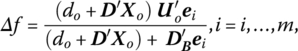
where the (m × 1) vector DB contains the coefficients of D corresponding to basic variables and ei is the ith unit column vector (Martos 1964; Kydland 1962; Bitran and Magnanti 1976).
In view of this discussion, the change in f per unit change in b1 is
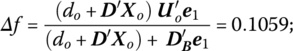
while the change in f per unit change in b2 is

13.9 Game Theory and Linear Programming
13.9.1 Introduction
We may view the notion of a game of strategy as involving a situation in which there is a contest or conflict situation between two or more players, where it is assumed that the players can influence the final outcome of the game, and the said outcome is not governed entirely by chance factors. The players can be individuals (two people engaging in a chess match, or multiple individuals playing a game of bridge) or, in a much broader sense, adversarial situations can emerge in a social, political, economic, or military context. Simply stated, a game is a set of rules for executing plays or moves. For example, the rules state what moves can be made, when they are to be made and by whom; what information is available to each participant; what are the termination criteria for a play or move, and so on. Moreover, after each play ends, we need to specify the reward or payoff to each player.
If the game or contest involves two individuals, organizations, or countries, it is called a two‐person game. And if the sum of the payoffs to all players at the termination of the game is zero, then the game is said to be a zero‐sum game, i.e. what one player wins, the other player loses. Hence a zero‐sum, two‐person game is one for which, at the end of each play, one player gains what the other player loses.
Suppose we denote the two players of a game as P1 and P2, respectively. Each player posits certain courses of action called strategies, i.e. these strategies indicate what one player will do for each possible move that his opponent might make. In addition, each player is assumed to have a finite number of strategies, where the number of strategies formulated by one player need not be the same for the other player. Hence the set of strategies for, say P1 covers all possible alternative ways of executing a play of the game given all possible moves that P2 might make.
It must be noted that for two‐person games, one of the opponents can be nature so that chance influences certain moves (provided, of course, that the players themselves ultimately control the outcome). However, if nature does not influence any moves and both parties select a strategy, then we say that the outcome of the game is strictly dominated. But if nature has a hand in affecting pays and the outcome of a game is not strictly determined, then it makes sense to consider the notion of expected outcome (more on this point later on).
13.9.2 Matrix Games
Let us specify a two‐person game G as consisting of the nonempty sets R and C and a real‐valued function ϕ defined on a pair (r, c), where r∈ ℛ and c∈ C. Here the elements r, c of sets R, C are the strategies for player P1 and P2, respectively, and the function ϕ is termed the payoff function. The number ϕ (r, c) is the amount that P2 pays P1 when P1 plays strategy r and P2 plays strategy c. If the sets R are finite, then the payoff ϕ can be represented by a matrix so that the game is called a matrix game.
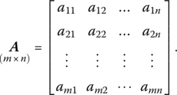
For matrix games, if R, C contain strategies r1, r2, …, rm and c1, c2, …, cn, respectively, then the payoff to P1 if he chooses strategy i and P2 selects strategy j is ϕ (ri, cj) = aij, i = 1, …, m; j = 1, …, n. If some moves are determined by chance, then the expected payoff to P1 is also denoted by aij. So when P1 chooses strategy i and P2 selects strategy j, aij depicts the payoff to P1 if the game is strictly determined or if nature makes some of the plays. In general, aij may be positive, negative, or zero. Given that P1 has m strategies and P2 has n strategies, the payoffs aij can be arranged into an (m × n) payoff matrix:
Clearly the rows represent the m strategies of P1 and the columns depict the n strategies of P2, where it is assumed that each player knows the strategies of his opponent. Thus, row i of A gives the payoff (or expected payoff) to P1 if he uses strategy i, with the actual payoff to P1 determined by the strategy selected by P2. A game is said to be in normal form if the strategies for each player are specified and the elements within A are given.
We can think of the aij elements of A as representing the payoffs to P1 while the payoffs to P2 are the negatives of these. The “conflict of interest” aspect of a game is easily understood by noting that P1 is trying to win as much as possible, with P2 trying to preclude P1 from winning more than is practicable. In this case, P1 will be regarded as the maximizing player while P2 will try to minimize the winnings of P1.
Given that P1 selects strategy i, he is sure of winning ![]() . (If “nature” impacts some of the moves, then P1’s expected winnings are at least
. (If “nature” impacts some of the moves, then P1’s expected winnings are at least ![]() aij.) Hence P1 should select the strategy that yields the maximum of these minima, i.e.
aij.) Hence P1 should select the strategy that yields the maximum of these minima, i.e.
Since it is reasonable for P2 to try to prevent P1 from getting any more than is necessary, selecting strategy j ensures that P1 will not get more than ![]() no matter what P1 does. Hence, P2 attempts to minimize his maximum loss, i.e. P2 selects a strategy for which
no matter what P1 does. Hence, P2 attempts to minimize his maximum loss, i.e. P2 selects a strategy for which
The strategies ri, i = 1, …, m, and cj, j = 1, …, n, are called pure strategies. Suppose P1 selects the pure strategy rl and P2 selects the pure strategy ck. If
then the game is said to possess a saddle point solution. Here rl turns out to be the optimal strategy for P1 while ck is the optimal strategy for P2 – with P2 selecting ck, P1 cannot get more than alk, and with P1 choosing rl, he is sure of winning at least alk.
Suppose (13.43) does not hold and that, say,
In this circumstance, P1 might be able to do better than arv, and P2 might be able to decrease the payoff to P1 below the auk level. For each player to pursue these adjustments, we must abandon the execution of pure strategies and look to the implementation of mixed strategies via a chance device. For P1, pure strategy i with probability ui ≥ 0 and ![]() is randomly selected; and for P2, pure strategy j with probability
is randomly selected; and for P2, pure strategy j with probability ![]() is randomly chosen. (More formally, a mixed strategy for P1 is a real‐valued function f on ℛ such that f(ri) = ui ≥ 0, while a mixed strategy for P2 is a real‐valued function h on C such that h(cj) = vj ≥ 0.) Thus random selection determines the strategy each player will use, and neither is cognizant of the other's strategy or even of his own strategy until it is determined by chance. In sum:
is randomly chosen. (More formally, a mixed strategy for P1 is a real‐valued function f on ℛ such that f(ri) = ui ≥ 0, while a mixed strategy for P2 is a real‐valued function h on C such that h(cj) = vj ≥ 0.) Thus random selection determines the strategy each player will use, and neither is cognizant of the other's strategy or even of his own strategy until it is determined by chance. In sum:
| or | or |
Under a regime of mixed strategies, we can no longer be sure what the outcome of the game will be. However, we can determine the expected payoff to P1. So if P1 uses mixed strategy U and P2 employs mixed strategy V, then the expected payoff to P1 is
Using an argument similar to that used to rationalize (13.41) and (13.42), P1 seeks a U that maximizes his expected winnings. For any U chosen, he is sure that his expected winnings will be at least ![]() P1 then maximizes his payoff relative to U so that his expected winnings are at least
P1 then maximizes his payoff relative to U so that his expected winnings are at least
Likewise, P2 endeavors to find a V such that the expected winnings of P1 do not exceed
Now, if there exist mixed strategies U*, V* such that ![]() then there exists a generalized saddle point of ϕ (U,V). P1 should use the mixed strategy U* and P2 the mixed strategy V* so that the expected payoff to P1 is exactly
then there exists a generalized saddle point of ϕ (U,V). P1 should use the mixed strategy U* and P2 the mixed strategy V* so that the expected payoff to P1 is exactly ![]() the value of the game. How do we know that mixed strategies U, V exist such that the value of the game is
the value of the game. How do we know that mixed strategies U, V exist such that the value of the game is ![]() The answer is provided by Theorem 13.7.
The answer is provided by Theorem 13.7.
13.9.3 Transformation of a Matrix Game to a Linear Program
Let us express a matrix game for players P1 and P2 as
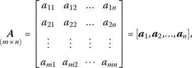
where aj, j = 1, …, n, is the jth column of A. Suppose P2 chooses to play the pure strategy j. If P1 uses the mixed strategy U ≥ O, 1′U = 1, then the expected winnings of P1 is
Then P1’s expected payoff will be at least W1 if there exists a mixed strategy U such that
i.e. P1 can never expect to win more than the largest value of W1 for which there exists a U > O, 1′U = 1, and (13.48) holds. Considering each j, (13.47) becomes
With W1 assumed to be positive, we can set
Clearly yi > 0 since W1 > 0. Under this variable, transformation (13.49) can be rewritten as
Here P1’s decision problem involves solving the linear program

Thus, minimizing ![]() will yield the maximum value of W1, the expected winnings for P1.
will yield the maximum value of W1, the expected winnings for P1.
Next, suppose P1 decides to play pure strategy i. From the viewpoint of P2, he attempts to find a mixed strategy V ≥ O 1′V = 1, which will give the smallest W2 such that, when P1 plays strategy i,
where αi is the ith row of the payoff matrix A and E(αiV) is the expected payout of P2. Considering each i, (13.53) becomes
With W2 taken to be positive, let us define
Hence (13.54) becomes
Thus P2’s decision problem is a linear program of the form

i.e. maximizing ![]() will yield the minimum value of W2, the upper bound on the expected payout of P2.
will yield the minimum value of W2, the upper bound on the expected payout of P2.
A moment’s reflection reveals that (13.57) can be called the primal problem and (13.52) is its symmetric dual. Moreover, from our previous discussion of duality theory, there are always feasible solutions U, V since P1, P2 can execute pure strategies. And with W1, W2 each positive, there exist feasible vectors X, Y for the primal and dual problems, respectively, and thus the primal and dual problems have optimal solutions with max z′ = min z or
These observations thus reveal that we have actually verified the fundamental theorem of game theory by constructing the primal‐dual pair of linear programs for P1 and, P2.
13.A Quadratic Forms
13.A.1 General Structure
Suppose Q is a function of the n variables x1, …, xn. Then Q is termed a quadratic form in x1, …, xn if
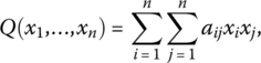
where at least one of the constant coefficients aij ≠ 0. More explicitly,

It is readily seen that Q is a homogeneous4 polynomial of the second degree since each term involves either the square of a variable or the product of two different variables. Moreover, Q contains n2 distinct terms and is continuous for all values of the variables xi, i = 1, …, n, and equals zero when xi = 0 for all i = 1, …, n.
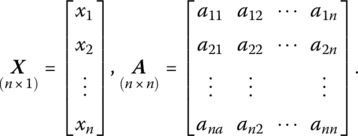
In matrix form Q equals, for X∈ En, the scalar quantity
where
To see this, let us first write
Then

From (13.A.2) it can be seen that aij + aji is the coefficient of xixj since aij, aji are both coefficients of xixj = xjxi, i ≠ j.
13.A.2 Symmetric Quadratic Forms
Remember that if a matrix A is symmetric so that A = A′, then aij = aji, i ≠ j. In this regard, a quadratic form X′AX is symmetric if A is symmetric or aij = aji, i ≠ j. Hence aij + aji = 2aij is the coefficient on xixj since aij = aji and aij, aji are both coefficients of xij = xji, i ≠ j.
If A is not a symmetric matrix (aij ≠ aji), we can always transform it into a symmetric matrix B by defining new coefficients
Then bij + bji = 2bij is the coefficient of xixj, i ≠ j, in

(Since bij + bji = ai + aij, this redefinition of coefficients clearly leaves the value of Q unchanged and thus, under (13.A.4), X′AX = X′BX, X∈ En.) So given any quadratic form X′AX, the matrix A may be assumed to be symmetric. If it is not, it can be readily transformed into a symmetric matrix.
13.A.3 Classification of Quadratic Forms
As we shall now see, there are, in all, five mutually exclusive and collectively exhaustive varieties of quadratic forms. Specifically:
- Definite Quadratic Form
A quadratic form is said to be positive definite (negative definite) if it is positive (negative) at every point X∈ En except X = O. That is
- X′AX is positive definite if X′AX > 0 for every X ≠ O;
- X′AX is negative definite if X′AX < 0 for every X ≠ O.
(Clearly a form that is either positive or negative definite cannot assume both positive and negative values.)
- Semi‐Definite Quadratic Form
A quadratic form is said to be positive semi‐definite (negative semi‐definite) if it is nonnegative (nonpositive) at every point X∈ En, and there exist points X ≠ O for which it is zero. That is:
- X′AX is positive semi‐definite if X′AX ≥ 0 for every X and X′AX = 0 for some points X ≠ O;
- X′AX is negative semi‐definite if X′AX ≤ 0 for every X and X′AX = 0 for some points X ≠ O.
- Indefinite Quadratic Forms
A quadratic form is said to be indefinite if it is positive for some points X∈ En and negative for others.
13.A.4 Necessary Conditions for the Definiteness and Semi‐Definiteness of Quadratic Forms
We now turn to an assortment of theorems (13.A.1–13.A.3) that will enable us to identify the various types of quadratic forms.
Note that the converse of this theorem does not hold since a quadratic form may have positive (negative) coefficients on all its terms involving second powers yet not be definite, e.g. ![]() Similarly,
Similarly,
(Here, too, the converse of the theorem is not true, e.g. the quadratic form ![]() has nonnegative coefficients associated with its second‐degree terms, yet is indefinite.)
has nonnegative coefficients associated with its second‐degree terms, yet is indefinite.)
Before stating our next theorem, let us define the kth naturally ordered principal minor of A as

or

In the light of this definition, we now look to
So, if any Mk = 0, k = 1, …, n, the form is not definite – but it may be semi‐definite or indefinite.
13.A.5 Necessary and Sufficient Conditions for the Definiteness and Semi‐Definiteness of Quadratic Forms
Let us modify Theorem 13.A.3 so as to obtain Theorem 13.A.4.
We next have Theorem 13.A.5.
A similar set of theorems (13.A.6 and 13.A.7) holds for semi‐definite quadratic forms. Specifically,
Similarly,