12
Duality Revisited
12.1 Introduction
The material presented in this chapter is largely theoretical in nature and may be considered to be a more “refined” approach to the study of linear programming and duality. That is to say, the mathematical techniques employed herein are quite general in nature in that they encompass a significant portion of the foundations of linear (as well as nonlinear) programming. In particular, an assortment of mathematical concepts often encountered in the calculus, along with the standard matrix operations which normally underlie the theoretical development of linear programming, are utilized to derive the Karush‐Kuhn‐Tucker necessary conditions for a constrained extremum and to demonstrate the formal equivalence between a solution to the primal maximum problem and the associated saddle‐point problem. Additionally, the duality and complementary slackness theorems of the preceding chapter are reexamined in the context of this “alternative” view of the primal and dual problems.
12.2 A Reformulation of the Primal and Dual Problems
Turning to the primal problem, let us maximize f(X) = C′X subject to AX ≤ b, X ≥ O, X ∈ En, where A is of order (m × n) with rows a1, …, am, and b is an (m × 1) vector with components b1, …, bm. Alternatively, if
are, respectively, of order (m + n × n) and (m + n × 1), then we may maximize f(X) = C′X subject to ![]() where X ∈ En is now unrestricted. In this formulation xj ≥ 0, j = 1, …, n, is treated as a structural constraint so that
where X ∈ En is now unrestricted. In this formulation xj ≥ 0, j = 1, …, n, is treated as a structural constraint so that ![]() defines a region of feasible or admissible solutions ⊆ En.
defines a region of feasible or admissible solutions ⊆ En.
If X0 yields an optimal solution to the primal maximum problem, then no permissible change in X (i.e. one that does not violate any of the constraints specifying K) can improve the optimal value of the objective function. How may we characterize such admissible changes? It is evident that, if starting at some feasible X, we can find a vector h such that a small movement along it violates no constraint, then h specifies a feasible direction at X. More formally, let δ(X0) be a suitably restricted spherical δ – neighborhood about the point X0 ∈ En. Then the (n × 1) vector h is a feasible direction at X0 if there exists a scalar t ≥ 0, 0 ≤ t < δ, such that X0 + th is feasible. In this light, for δ(X0) again a spherical δ − neighborhood about the feasible point X0 ∈ En, the set of feasible directions at X0, D(X0), is the collection of all (n × 1) vectors h such that X0 + th is feasible for t sufficiently small, i.e.
Here D(X0) is the tangent support cone consisting of all feasible directions at X0 and is generated by the tangent or supporting hyperplanes to K at X0 (Figure 12.1). And since each such hyperplane
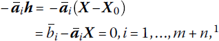
Figure 12.1 Set of feasible directions D(X0).
specifies a closed half‐space ![]() the tangent support cone D(X0) represents that portion of the intersection of these closed half‐planes in the immediate vicinity of (X0).
the tangent support cone D(X0) represents that portion of the intersection of these closed half‐planes in the immediate vicinity of (X0).
To discern the relationship between D(X0)(X0 optimal) and: (i) f(X0); (ii) the constraints ![]() let us consider the following two theorems, starting with Theorem 12.1.
let us consider the following two theorems, starting with Theorem 12.1.
Hence f must decrease along any feasible direction h. Geometrically, no feasible direction may form an acute angle (<π/2) between itself and C.
To set the stage for our next theorem, we note that for any optimal X∈ K, it is usually the case that not all the inequality constraints are binding or hold as an equality. To incorporate this observation into our discussion, let us divide all of the constraints ![]() into two mutually exclusive classes – those that are binding at
into two mutually exclusive classes – those that are binding at ![]() and those which are not,
and those which are not, ![]() So if
So if
depicts the index set of binding constraints, then ![]() for i ∉ I. In this regard, we have Theorem 12.5.
for i ∉ I. In this regard, we have Theorem 12.5.
To interpret this theorem, we note that ![]() may be characterized as an inward pointing or interior normal to
may be characterized as an inward pointing or interior normal to ![]() at X0. So if h is a feasible direction, it makes a nonobtuse angle (≤π/2) with all of the interior normals to the boundary of K at X0. Geometrically, these interior normal or gradients of the binding constraints form a finite cone containing all feasible directions making nonobtuse angles with the supporting hyperplanes to K at X0. Such a cone is polar to the tangent support cone D(X0) and will be termed the polar support cone D(X0)+(Figure 12.2a) Thus, D(X0)+ is the cone spanned by the gradients
at X0. So if h is a feasible direction, it makes a nonobtuse angle (≤π/2) with all of the interior normals to the boundary of K at X0. Geometrically, these interior normal or gradients of the binding constraints form a finite cone containing all feasible directions making nonobtuse angles with the supporting hyperplanes to K at X0. Such a cone is polar to the tangent support cone D(X0) and will be termed the polar support cone D(X0)+(Figure 12.2a) Thus, D(X0)+ is the cone spanned by the gradients ![]() such that for h∈D
such that for h∈D ![]() i ∈ J. Looked at from another perspective,
i ∈ J. Looked at from another perspective, ![]() may be considered an outward‐pointing or exterior normal to the boundary of K at X0. In this instance, if h is a feasible direction, it must now make a non‐acute angle (≥π/2) with all of the outward‐pointing normals to the boundary of K at X0. Again looking to geometry, the exterior normals or negative gradients of the binding constraints form a finite cone containing all feasible directions making nonacute angles with the hyperplanes tangent to K at X0. This cone is the dual of the tangent support cone D(X0) and is termed the dual support cone D(X0)*(Figure 12.2b). Thus, D(X0)* is the cone spanned by the negative gradients
may be considered an outward‐pointing or exterior normal to the boundary of K at X0. In this instance, if h is a feasible direction, it must now make a non‐acute angle (≥π/2) with all of the outward‐pointing normals to the boundary of K at X0. Again looking to geometry, the exterior normals or negative gradients of the binding constraints form a finite cone containing all feasible directions making nonacute angles with the hyperplanes tangent to K at X0. This cone is the dual of the tangent support cone D(X0) and is termed the dual support cone D(X0)*(Figure 12.2b). Thus, D(X0)* is the cone spanned by the negative gradients ![]() such that, for all h∈D
such that, for all h∈D ![]() i ∈ J.
i ∈ J.
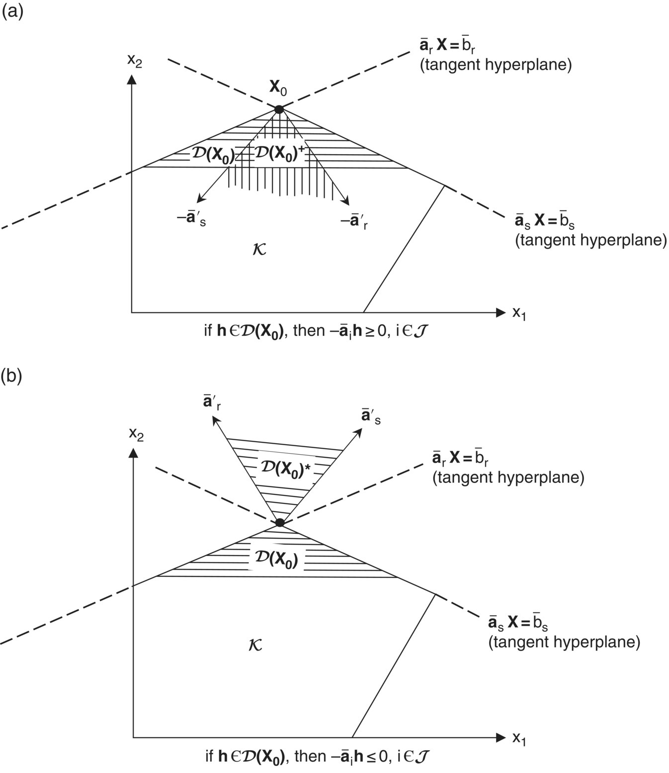
Figure 12.2 (a) Polar support cone D(X0)+; (b) Dual support cone D(X0)*.
At this point, let us collect our major results. We found that if f(X) subject to ![]() i ∈ J, attains its maximum at X0, then
i ∈ J, attains its maximum at X0, then
How may we interpret this condition? Given any h∈ D(X0), (12.1) holds if the gradient of f or C lies within the finite cone spanned by the exterior normals ![]() i ∈ J, i.e. C∈ D(X0)*(or if −C is contained within the finite cone generated by the interior normals
i ∈ J, i.e. C∈ D(X0)*(or if −C is contained within the finite cone generated by the interior normals ![]() i ∈ J, i.e. −C∈ D(X0)+). Hence (12.1) requires that the gradient of f be a nonnegative linear combination of the negative gradients of the binding constraints at X0 (Figure 12.3). In this regard, there must exist real numbers
i ∈ J, i.e. −C∈ D(X0)+). Hence (12.1) requires that the gradient of f be a nonnegative linear combination of the negative gradients of the binding constraints at X0 (Figure 12.3). In this regard, there must exist real numbers ![]() such that
such that
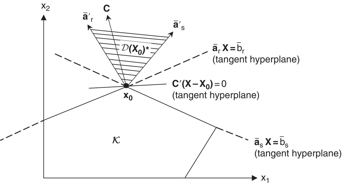
Figure 12.3 C ∈ D(X0)*.
Under what conditions will the numbers ![]() , i ∈ J, exist? To answer this question, let us employ Theorem 12.3.
, i ∈ J, exist? To answer this question, let us employ Theorem 12.3.
Returning now to our previous question, in terms of the notation used above, if: C = V; the vectors ![]() i ∈ J, are taken to be the columns of B (i.e.
i ∈ J, are taken to be the columns of B (i.e. ![]() ); and the
); and the ![]() i ∈ J, are the elements of λ ≥ O, then a necessary and sufficient condition for C to lie within the finite cone generated by the vectors
i ∈ J, are the elements of λ ≥ O, then a necessary and sufficient condition for C to lie within the finite cone generated by the vectors ![]() is that C′h ≤ 0 for all h satisfying
is that C′h ≤ 0 for all h satisfying ![]() i ∈ J. Hence, there exist real numbers
i ∈ J. Hence, there exist real numbers ![]() such that (12.2) holds.
such that (12.2) holds.
We may incorporate all of the constraints (active or otherwise) ![]() into our discussion by defining the scalar
into our discussion by defining the scalar ![]() as zero whenever
as zero whenever ![]() or i ∉ J. Then (12.2) is equivalent to the system
or i ∉ J. Then (12.2) is equivalent to the system
where ![]() Note that
Note that ![]() for all i values since, if
for all i values since, if ![]() then
then ![]() while if
while if ![]() then
then ![]()
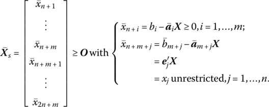
When we formed the structural constraint inequality ![]() the n non‐negativity conditions X ≥ O were treated as structural constraints. That is, xj ≥ 0 was converted to
the n non‐negativity conditions X ≥ O were treated as structural constraints. That is, xj ≥ 0 was converted to ![]() However, if the non‐negativity conditions are not written in this fashion, but appear explicitly as X ≥ O, then (12.3) may be rewritten in an equivalent form provided by Theorem 12.4.
However, if the non‐negativity conditions are not written in this fashion, but appear explicitly as X ≥ O, then (12.3) may be rewritten in an equivalent form provided by Theorem 12.4.
We note briefly that if the primal problem appears as
Then (12.4) becomes
We now turn to a set of important corollaries to the preceding theorem (Corollaries 12.1, 12.2, and 12.3).
Next,
Finally,
So if the right‐hand side bi of the ith primal structural constraint were changed by a sufficiently small amount εi, then the corresponding change in the optimal value of f, f0, would be ![]() Moreover, since
Moreover, since ![]() we may determine the amount by which the optimal value of the primal objective function changes given small (marginal) changes in the right‐hand sides of any specific subset of structural constraints. For instance, let us assume, without loss of generality, that the right‐hand sides of the first t < m primal structural constraints are increased by sufficiently small increments ε1, …, εt, respectively. Then the optimal value of the primal objective function would be increased by
we may determine the amount by which the optimal value of the primal objective function changes given small (marginal) changes in the right‐hand sides of any specific subset of structural constraints. For instance, let us assume, without loss of generality, that the right‐hand sides of the first t < m primal structural constraints are increased by sufficiently small increments ε1, …, εt, respectively. Then the optimal value of the primal objective function would be increased by ![]()
Throughout the preceding discussion the reader may have been wondering why the qualification “generally” was included in the statement of Corollary 12.3. The fact of the matter is that there exist values of, say, bk, for which ∂f0/∂bk is not defined, i.e. points where ∂f0/∂bk is discontinuous so that (12.10) does not hold. To see this, let us express f in terms of bk, as
where the ![]() depict fixed levels of the requirements
depict fixed levels of the requirements ![]() .
.
If in Figure 12.4 we take area OABCG to be the initial feasible region when ![]() (here the line segment CG consists of all feasible points X that satisfy
(here the line segment CG consists of all feasible points X that satisfy ![]() , then increasing the kth requirement from
, then increasing the kth requirement from ![]() changes the optimal extreme point from C to D. The result of this increase in bk is a concomitant increase in f0 proportionate to the distance
changes the optimal extreme point from C to D. The result of this increase in bk is a concomitant increase in f0 proportionate to the distance ![]() where the constant of proportionality is
where the constant of proportionality is ![]() Thus, over this range of bk values, ∂f0/∂bk exists (is continuous). If we again augment the level of bk by the same amount as before, this time shifting the kth structural constraint so that it passes through point E, ∂f0/∂bk becomes discontinuous since now the maximal point moves along a more steeply sloping portion (segment EF) of the boundary of the feasible region so that any further equal parallel shift in the kth structural constraint would produce a much larger increment in the optimal value of f than before. Thus, each time the constraint line akX = bk passes through an extreme point of the feasible region, there occurs a discontinuity in ∂f0/∂bk.
Thus, over this range of bk values, ∂f0/∂bk exists (is continuous). If we again augment the level of bk by the same amount as before, this time shifting the kth structural constraint so that it passes through point E, ∂f0/∂bk becomes discontinuous since now the maximal point moves along a more steeply sloping portion (segment EF) of the boundary of the feasible region so that any further equal parallel shift in the kth structural constraint would produce a much larger increment in the optimal value of f than before. Thus, each time the constraint line akX = bk passes through an extreme point of the feasible region, there occurs a discontinuity in ∂f0/∂bk.
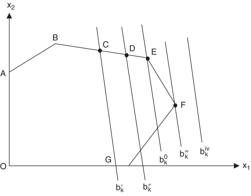
Figure 12.4 Increasing the requirements of bk.
To relate this argument directly to f(bk) above, let us describe the behavior of f(bk) as bk assumes the values ![]() In Figure 12.5 the piecewise continuous curve f(bk) indicates the effect on f(bk) precipitated by changes in bk. (Note that each time the constraint akX = bk passes through an extreme point of the feasible region in Figure 12.4, the f(bk) curve assumes a kink, i.e. a point of discontinuity in its derivative. Note also that for a requirement level of
In Figure 12.5 the piecewise continuous curve f(bk) indicates the effect on f(bk) precipitated by changes in bk. (Note that each time the constraint akX = bk passes through an extreme point of the feasible region in Figure 12.4, the f(bk) curve assumes a kink, i.e. a point of discontinuity in its derivative. Note also that for a requirement level of ![]() [say
[say ![]() ], f cannot increase any further so that beyond F′, f(bk) is horizontal) As far as the dual objective function g(u) = b′u is concerned, g may be expressed as g(bk) = bkuk+ constant since
], f cannot increase any further so that beyond F′, f(bk) is horizontal) As far as the dual objective function g(u) = b′u is concerned, g may be expressed as g(bk) = bkuk+ constant since ![]() is independent of bk. For
is independent of bk. For ![]() (
(![]() optimal),
optimal), ![]() Moreover, since the dual structural constraints are unaffected by changes in bk, dual feasibility is preserved for variations in bk away from
Moreover, since the dual structural constraints are unaffected by changes in bk, dual feasibility is preserved for variations in bk away from ![]() so that, in general, for any pair of feasible solutions to the primal and dual problems, f(bk) ≤ g(bk), i.e. g(bk) is tangent to f(bk) for
so that, in general, for any pair of feasible solutions to the primal and dual problems, f(bk) ≤ g(bk), i.e. g(bk) is tangent to f(bk) for ![]() (point E′ in Figure 12.5) while
(point E′ in Figure 12.5) while ![]() sufficiently small. In this regard, for
sufficiently small. In this regard, for ![]() while for
while for ![]() whence
whence ![]() So while both the left‐ and right‐hand derivatives of f(bk) exist at
So while both the left‐ and right‐hand derivatives of f(bk) exist at ![]() itself does not exist since
itself does not exist since ![]() i.e. ∂f/∂bk possesses a finite discontinuity at
i.e. ∂f/∂bk possesses a finite discontinuity at ![]() . In fact, ∂f/∂bk is discontinuous at each of the points, A′, B′, E′ and F′ in Figure 12.5. For
. In fact, ∂f/∂bk is discontinuous at each of the points, A′, B′, E′ and F′ in Figure 12.5. For ![]() it is evident that
it is evident that ![]() since f(bk), g(bk) coincide all along the segment B′ E′ of Figure 12.5. In this instance, we may unequivocally write
since f(bk), g(bk) coincide all along the segment B′ E′ of Figure 12.5. In this instance, we may unequivocally write ![]() Moreover, for
Moreover, for ![]() (see Figures 12.4 and 12.5),
(see Figures 12.4 and 12.5), ![]() since the constraint
since the constraint ![]() is superfluous, i.e. it does not form any part of the boundary of the feasible region. In general, then, ∂f/∂bk|+ ≤ uk ≤ ∂f/∂bk|−.
is superfluous, i.e. it does not form any part of the boundary of the feasible region. In general, then, ∂f/∂bk|+ ≤ uk ≤ ∂f/∂bk|−.
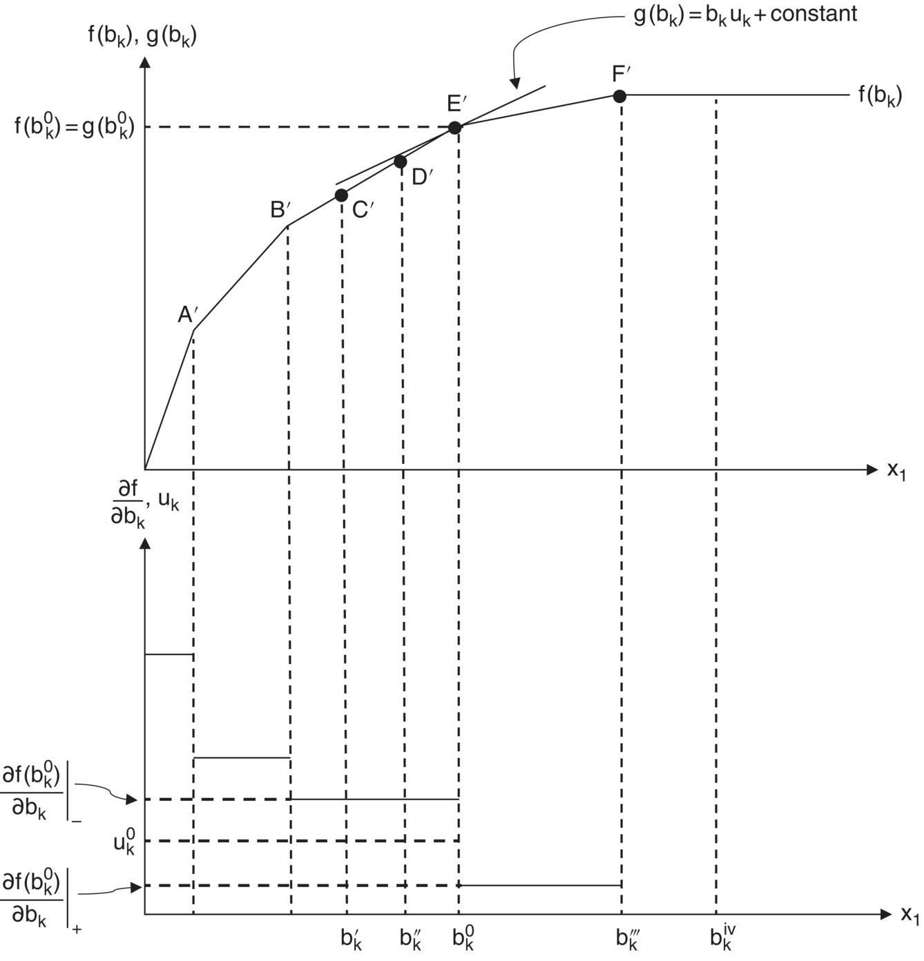
Figure 12.5 Tracking f(bk) as bk increases.
To formalize the preceding discussion, we state Theorem 12.5.
To summarize: if both the left‐ and right‐hand derivatives ∂f0/∂bi|−, ∂f0/∂bi|+ exist and their common value is ![]() then
then ![]() otherwise
otherwise ![]()
12.3 Lagrangian Saddle Points
(Belinski and Baumol 1968; Williams 1963)
If we structure the primal‐dual pair of problems as
PRIMAL PROBLEM |
DUAL PROBLEM |
then the Lagrangian associated with the primal problem is L(X, U) = C′X + U′(b − AX) with X ≥ O, U ≥ O. And if we now express the dual problem as maximize {−b′U} subject to −A′U ≤ − C,U ≥ O, then the Lagrangian of the dual problem is M(U, X) = − b′U + X′(−C + A′U), where again U ≥ O, X ≥ O. Moreover, since M(U, X) = − b′U + X′C + X′A′U = − C′X − U′b + U′AX = − L(X, U), we see that the Lagrangian of the dual problem is actually the negative of the Lagrangian of the primal problem. Alternatively, if xj ≥ 0 is converted to ![]() then the revised primal problem appears as
then the revised primal problem appears as

with associated Lagrangian ![]() where
where ![]() As far as the dual of this revised problem is concerned, we seek to
As far as the dual of this revised problem is concerned, we seek to

In this instance ![]() also.
also.
We next turn to the notion of a saddle point of the Lagrangian. Specifically, a point (X0, Uo)ε En + m is termed a saddle point of the Lagrangian L(X, U) = C′X + U′(b − AX) if
for all X ≥ O, U ≥ O. Alternatively, ![]() E2n + m is a saddle point of
E2n + m is a saddle point of ![]() if
if
for all X unrestricted and U ≥ O. What these definitions imply is that ![]() simultaneously attains a maximum with respect to X and a minimum with respect to
simultaneously attains a maximum with respect to X and a minimum with respect to ![]() Hence (12.11), (12.12) appear, respectively, as
Hence (12.11), (12.12) appear, respectively, as
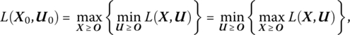

Under what conditions will ![]() possess a saddle point at
possess a saddle point at ![]() To answer these questions, we must look to the solution of what may be called the saddle point problem: To find a point (X0, U0) such that (12.11) holds for all (X, U)ε En + m, X ≥ O, U ≥ O; or, to find a point
To answer these questions, we must look to the solution of what may be called the saddle point problem: To find a point (X0, U0) such that (12.11) holds for all (X, U)ε En + m, X ≥ O, U ≥ O; or, to find a point ![]() such that (12.12) holds for all
such that (12.12) holds for all ![]() E2n + m, X unrestricted,
E2n + m, X unrestricted, ![]()
In the light of (12.11.1), (12.12.1) we shall ultimately see that determining a saddle point of a Lagrangian corresponds to maxi‐minimizing or mini‐maximizing it. To this end, we look to Theorem 12.6.
Our discussion in this chapter has centered around the solution of two important types of problems – the primal linear programming problem and the saddle point problem. As we shall now see, there exists an important connection between them. Specifically, what does the attainment of a saddle point of the Lagrangian of the primal problem imply about the existence of a solution to the primal problem? To answer this, we cite Theorem 12.7.
The importance of the developments in this section is that they set the stage for an analysis of the Karush‐Kuhn‐Tucker equivalence theorem. This theorem (Theorem 12.5) establishes the notion that the existence of an optimal solution to the primal problem is equivalent to the existence of a saddle point of its associated Lagrangian, i.e. solving the primal problem is equivalent to maxi‐minimizing (mini‐maximizing) its Lagrangian.
It is instructive to analyze this equivalence from an alternative viewpoint. We noted above that solving the primal linear programming problem amounts to maxi‐minimizing (mini‐maximizing) its associated Lagrangian. In this regard, if we express the primal problem as

then, if L(X, U0) has a maximum in the X‐ direction at X0, it follows from (12.4a, b, f) that

while, if L(X0, U) attains a minimum in the U‐ direction at U0, then, from (12.4c, d, e),

Thus, X0 is an optimal solution to the preceding primal problem if and only if there exists a vector U0 ≥ O such that (X0, U0) is a saddle point of L(X, U), in which case system (12.4) is satisfied.
One final point is in order. As a result of the discussion underlying the Karush‐Kuhn‐Tucker equivalence theorem, we have Corollary 12.4.
12.4 Duality and Complementary Slackness Theorems
(Dreyfus and Freimer 1962)
We now turn to an alternative exposition of two of the aforementioned fundamental theorems of linear programming (Chapter 6), namely the duality and complementary slackness theorems. First, Theorem 12.5 explains the duality theorem.
Next, if, as above, we express the primal‐dual pair of problems as
PRIMAL PROBLEM |
DUAL PROBLEM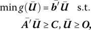 |
then their associated Lagrangians may be written, respectively, as
where ![]() is an (m + n × 1) vector of nonnegative primal slack variables, i.e.
is an (m + n × 1) vector of nonnegative primal slack variables, i.e.
In this light, we now look to Theorem 12.5.
By way of interpretation: (i) if the primal slack variable ![]() corresponding to the ith primal structural constraint is positive, then the associated dual variable
corresponding to the ith primal structural constraint is positive, then the associated dual variable ![]() must equal zero. Conversely, if
must equal zero. Conversely, if ![]() is positive, then the ith primal structural constraint must hold as an equality with
is positive, then the ith primal structural constraint must hold as an equality with ![]() Before turning to point (ii), let us examine the form of the jth dual structural constraint. Since A = [α1, …, αn],
Before turning to point (ii), let us examine the form of the jth dual structural constraint. Since A = [α1, …, αn],

and thus the jth dual structural constraint appears as ![]() In this light, (ii) if the jth primal variable
In this light, (ii) if the jth primal variable ![]() is different from zero, then the dual surplus variable
is different from zero, then the dual surplus variable ![]() associated with the jth dual structural constraint
associated with the jth dual structural constraint ![]() equals zero. Conversely, if
equals zero. Conversely, if ![]() then the jth dual structural constraint is not binding and thus the jth primal variable
then the jth dual structural constraint is not binding and thus the jth primal variable ![]() must be zero.
must be zero.