6.1 The Symmetric Dual

Given a particular linear programming problem, there is associated with it another (unique) linear program called its dual. In general, duality theory addresses itself to the study of the connection between two related linear programming problems, where one of them, the primal, is a maximization (minimization) problem and the other, the dual, is a minimization (maximization) problem. Moreover, this association is such that the existence of an optimal solution to any one of these two problems guarantees an optimal solution to the other, with the result that their extreme values are equal. To gain some additional insight into the role of duality in linear programming, we note briefly that the solution to any given linear programming problem may be obtained by applying the simplex method to either its primal or dual formulation, the reason being that the simplex process generates an optimal solution to the primal‐dual pair of problems simultaneously. So with the optimal solution to one of these problems obtainable from the optimal solution of its dual, there is no reason to solve both problems separately. Hence the simplex technique can be applied to whichever problem requires the least computational effort.

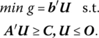
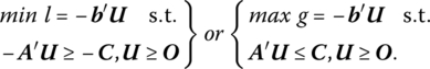
We now turn to the expression of the primal problem in canonical form and then look to the construction of its associated dual. Specifically, if the primal problem appears as

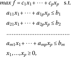
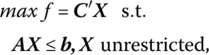
then its dual is

Henceforth, this form of the dual will be termed the symmetric dual, i.e. in this instance, the primal and dual problems are said to be mutually symmetric. In matrix form, the symmetric primal‐dual pair of problems appears as

Primal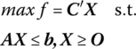

Symmetric Dual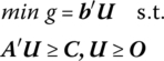

where X and C are of order (p × 1), U and b are of order (m × 1), and A is of order (m × p). In standard form, the primal and its symmetric dual may be written as

Primal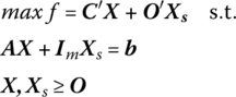

Symmetric Dual

where X_s, U_s denote (m × 1) and (p × 1) vectors of primal slack and dual surplus variables, respectively.

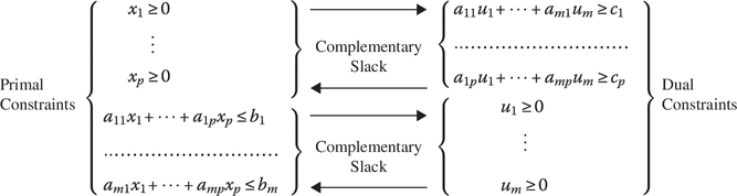
An examination of the structure of the primal and symmetric dual problems reveals the following salient features:

1. If the primal problem involves maximization, then the dual problem involves minimization, and conversely. A new set of variables appears in the dual.
2. In this regard, if there are p variables and m structural constraints in the primal problem, there will be m variables and p structural constraints in the dual problem, and conversely. In particular, there exists a one‐to‐one correspondence between the jth primal variable and the jth dual structural constraint, and between the ith dual variable and the ith primal structural constraint.
3. The primal objective function coefficients become the right‐hand sides of the dual structural constraints and, conversely. The coefficient matrix of the dual structural constraint system is the transpose of the coefficient matrix of the primal structural constraint system, and vice‐versa. Thus, the coefficients on x_j in the primal problem become the coefficients of the jth dual structural constraint.
4. The inequality signs in the structural constraints of the primal problem are reversed in the dual problem, and vice‐versa.

6.2 Unsymmetric Duals

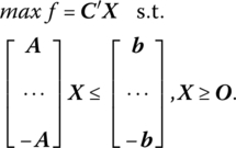
This section will develop a variety of duality relationships and forms that result when the primal maximum problem involves structural constraints other than of the “≤” variety and variables that are unrestricted in sign. In what follows, our approach will be to initially write the given primal problem in canonical form, and then, from it, obtain the corresponding symmetric dual problem. To this end, let us first assume that the primal problem appears as

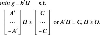
In this instance two sets of inequality structural constraints are implied by AX = b, i.e. AX ≤ b, − AX ≤  − b must hold simultaneously. Then the above primal problem has the canonical form

The symmetric dual associated with this problem becomes

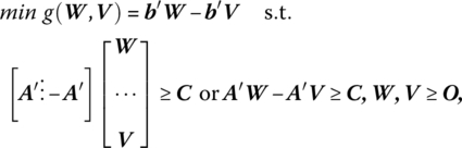
where the dual variables W, V are associated with the primal structural constraints AX ≤ b, −AX ≤ −b, respectively.

If U = W − V, then we ultimately obtain

since if both W, V ≥ O, their difference may be greater than or equal to, less than or equal to, or exactly equal to, the null vector.

Next, suppose the primal problem appears as

In canonical form, we seek to

The symmetric dual associated with this problem is

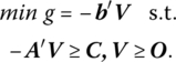
If U = −V, then we finally

Lastly, if the primal problem is of the form

then, with X expressible as the difference between the two vectors X₁, X₂ whose components are all nonnegative, the primal problem becomes

The symmetric dual of this latter problem is

To summarize, let us assume that the primal maximum problem contains a mixture of structural constraints. Then:

1. If the primal variables are all nonnegative, the dual minimum problem has the following properties:
   1. The form of the dual structural constraint system is independent of the form of the primal structural constraint system, i.e. the former always appears as A^′U ≥ C. Moreover, only the dual variables are influenced by the primal structural constraints. Specifically:
   2. The dual variable u_r corresponding to the rth “≤” primal structural constraint is nonnegative.
   3. The dual variable u_s corresponding to the sth “≥” primal structural constraint is nonpositive.
   4. The dual variable u_t corresponding to the tth “=” primal structural constraint is unrestricted in sign.
2. If some variable x_j in the primal problem is unrestricted in sign, then the jth dual structural constraint will hold as an equality.

6.3 Duality Theorems

To further enhance our understanding of the relationship between the primal and dual linear programming problems, let us consider the following sequence of duality theorems (Theorems 6.1–6.3).

The implication of this theorem is that it is immaterial which problem is called the dual.

The next two theorems address the relationship between the objective function values of the primal‐dual pair of problems. First,

In this regard, the dual objective function value provides an upper bound to the value of the primal objective function. Second,

In addition, either both the primal maximum and dual minimum problems have optimal vectors X₀, U₀, respectively, with C^′X₀ = b^′U₀, or neither has an optimal vector.

We noted in Chapter 4 that it is possible for the primal objective function to be unbounded over the feasible region K. What is the implication of this outcome as far as the behavior of the dual objective is concerned? As will be seen in Example 6.4, if the primal maximum (dual minimum) problem possesses a feasible solution and C^′X(b^′U) is unbounded from above (below), then the dual minimum (primal maximum) problem is infeasible. Looked at in another fashion, one (and thus both) of the primal maximum and dual minimum problems has an optimal solution if and only if either C^′X or b^′U is bounded on its associated nonempty feasible region.

We now turn to what may be called the fundamental theorems of linear programming. In particular, we shall examine the existence, duality, and complementary slackness theorems.

We first state Theorem 6.4.

We next have Theorem 6.5.

We now turn to the third fundamental theorem of linear programming, namely a statement of the complementary slackness conditions. Actually, two such theorems will be presented – the strong and the weak cases. We first examine the weak case provided by Theorem 6.6.

That is, for optimal solutions to the primal maximum and dual minimum problems, respectively:

1. If a primal slack variable is positive, then the ith dual variable must equal zero. Conversely, if is positive, then equals zero;
2. If the jth primal variable is positive, then the dual surplus variable equals zero. Conversely, if is positive, then must equal zero.

How may we interpret (6.1)? Specifically, implies that either and or and or both Similarly, implies that either and or and or both Alternatively, if the constraint system for the primal‐dual pair of problems is written as

and (6.1) is rewritten as

(6.1.1)

it is easily seen that if the kth dual variable is positive, then its complementary primal structural constraint is binding (i.e. holds as an equality). Conversely, if the kth primal structural constraint holds with strict inequality, then its complementary dual variable is zero. Likewise, if the lth primal variable is positive, then its complementary dual structural constraint is binding. Conversely, if the lth dual structural constraint holds as a strict inequality, its complementary primal variable is zero. In short, and as well as and are complementary slack since within each pair of inequalities at least one of them must hold as an equality.

As a final observation, the geometric interpretation of the weak complementary slackness conditions is that at an optimal solution to the primal‐dual pair of problems, the vector of primal variables X₀ is orthogonal to the vector of dual surplus variables (U_s)₀ while the vector of dual variables U₀ is orthogonal to the vector of primal slack variables (X_s)₀.

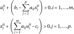
It is important to note that the weak complementary slackness conditions (6.1), (6.1.1) must hold for every pair of optimal solutions to the primal and dual problems. However, it may happen that, say, for some particular value of j (i), both vanish at the said solutions. In this instance, can we be sure that there exists at least one pair of optimal solutions to the primal and dual problems for which this cannot occur? The answer is in the affirmative, as Theorem 6.7 demonstrates.

By way of an interpretation: implies that either and or and but not both ; while , implies that either and or and but not both

Let us now establish the connection between the weak and strong complementary slackness conditions by first rewriting (6.2) as

(6.2.1)

Then, for the strong case, if the kth dual variable is zero, then its complementary primal structural constraint holds as a strict inequality. Conversely, if the kth primal structural constraint is binding, then its complementary dual variable is positive. Note that this situation cannot prevail under the weak case since if it does not follow that i.e. under the weak conditions implies that Similarly (again considering the strong case), if the lth primal variable is zero, it follows that its complementary dual structural constraint holds with strict inequality. Conversely, if the lth dual structural constraint is binding, it follows that its complementary primal variable is positive. Here, too, a comparison of the strong and weak cases indicates that, for the latter, if we may conclude that but not that as in the former.

To summarize:

Weak Complementary Slackness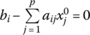 implies and implies while implies and implies

Strong Complementary Slackness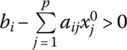 implies and implies while implies and implies

6.4 Constructing the Dual Solution

It was mentioned in the previous section that either both of the primal‐dual pair of problems have optimal solutions, with the values of their objective functions being the same, or neither has an optimal solution. Hence, we can be sure that if one of these problems possesses an optimal solution, then the other does likewise. In this light, let us now see exactly how we may obtain the optimal dual solution from the optimal primal solution. To this end, let us assume that the primal maximum problem

has an optimal basic feasible solution consisting of

As an alternative to expressing the optimal value of the primal objective function in terms of the optimal values of the primal basic variables x_Bi, i = 1, …, m, let us respecify the optimal value of the primal objective function in terms of the optimal dual variables by defining the latter as

(6.3)

where c_Bi, i = 1, …, m, is the ith component of C_B and β_ij, i, j = 1, …, m, is the element in the ith row and jth column of B⁻¹. Then f = U^′b so that the value of f corresponding to an optimal basic feasible solution may be expressed in terms of the optimal values of either the primal or dual variables. Moreover, if the primal optimality criterion is satisfied, the U is a feasible solution to the dual structural constraints. And since U is an optimal solution to the dual minimum given that X represents the optimal basic feasible solution to the primal maximum problem.

By way of an interpretation of these dual variables we have Theorem 6.8.

We noted earlier that the simplex method can be applied to either the primal or dual formulation of a linear programming problem, with the choice of the version actually solved determined by considerations of computational ease. In this regard, if the dual problem is selected, how may we determine the optimal values of the primal variables from the optimal dual solution? Given that the dual problem appears as

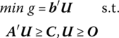
or

we may utilize the M‐penalty method to derive the artificial simultaneous augmented form

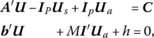
where U_a denotes an (m × 1) vector of nonnegative artificial variables and the associated simplex matrix is

Relative to this system the (p + 1 × p + 1) basis matrix and its inverse may be written, respectively, as

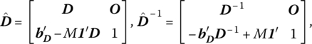
where D depicts the (m × m) basis matrix associated with the dual artificial structural constraint system. Then

(6.5)

yields a basic feasible solution to the dual minimum problem, where the vectors associated with the artificial variables, i.e. those corresponding to the third partitioned column of (6.5), have been deleted since the artificial vectors have been driven from the basis. If we assume that the optimality criterion is satisfied, then the optimal values of the primal variables appear as the circled array of elements in the objective function row of (6.5), i.e. X^′ = b_DD⁻¹ ≥ O^′. In addition, from the augmented primal structural constraint system AX + I_mX_s = b, we may isolate the primal slack variables as But this expression corresponds to the double‐circled array of elements in the objective function row of (6.5). To summarize, our rules for isolating the optimal values of the primal variables (original and slack) may be determined as follows:

1. To find the values of the primal variables X that correspond to an optimal basic feasible solution of the dual minimum problem, look in the last row of the final dual simplex matrix under those columns that were, in the original simplex matrix, the columns of the negative of the identity matrix. The jth primal variable x_j, j = 1, …, p, will appear under the column that was initially the jth column of the negative of the identity matrix.
2. To find the values of the primal slack variables X_s that correspond to an optimal basic feasible solution of the dual minimum problem, look in the last row of the final dual simplex matrix under those columns that were, in the original simplex matrix, the columns of the matrix A^′. The ith primal slack variable x_p + i, i = 1, …, m, will appear under the column that was initially the ith column of A^′.

In this section we have demonstrated how the dual (primal) variables may be obtained from the optimal primal (dual) simplex matrix. Hence, no matter which of the primal‐dual pair of problems is solved, all of the pertinent information generated by an optimal basic feasible solution is readily available, i.e. from either the final primal or dual simplex matrix we can isolate both the primal and dual original variables as well as the primal slack and dual surplus variables.

6.5 Dual Simplex Method (Lemke 1954)

In attempting to generate an optimal basic feasible solution to a linear programming problem, our procedure, as outlined in Chapters 4 and 5, was to employ the simplex method or, as we shall now call it, the primal simplex method. To briefly review this process, we start from an initial basic feasible solution for which the optimality criterion is not satisfied, i.e. not all (the dual problem is infeasible). We then make changes in the basis, one vector at a time, maintaining nonnegativity of the basic variables at each iteration until we obtain a basic feasible solution for which all (so that dual feasibility now holds). Hence the primal simplex method is a systematic technique that preserves primal feasibility while striving for primal optimality, thereby reducing, at each round, dual infeasibility, until primal optimality, and thus dual feasibility, is ultimately achieved. This last observation precipitates a very interesting question. Specifically, can we solve a linear programming problem by a procedure that works in a fashion opposite to that of the primal simplex algorithm? That is to say, by a method which relaxes primal feasibility while maintaining primal optimality. As we shall now see, the answer is yes. In this regard, we now look to an alternative simplex routine called the dual simplex method, so named because it involves an application of the simplex method to the dual problem, yet is constructed so as to have its pivotal operations carried out within the standard primal simplex matrix. Here the starting point is an initial basic but nonfeasible solution to the primal problem for which optimality (and thus dual feasibility) holds. As is the usual case, we move from this solution to an optimal basic feasible solution through a sequence of pivot operations which involve changing the status of a single basis vector at a time. Hence the dual simplex method preserves primal optimality (dual feasibility) while reducing, at each iteration, primal infeasibility, so that an optimal basic feasible solution to both the primal and dual problems is simultaneously achieved. Moreover, while the primal objective starts out at a suboptimal level and monotonically increases to its optimal level, the dual objective starts out at a superoptimal level and monotonically decreases to its optimal feasible value.

6.6 Computational Aspects of the Dual Simplex Method

One important class of problems that lends itself to the application of the dual simplex method is when the primal problem is such that a surplus variable is added to each “≥” structural constraint. As we shall see below, the dual simplex method enables us to circumvent the procedure of adding artificial variables to the primal structural constraints. For instance, if the primal problem appears as:

then the (symmetric) dual problem may be formed as

To determine an initial basic solution to the primal problem, let us examine its associated simplex matrix:

(6.6)

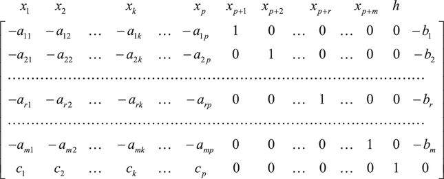
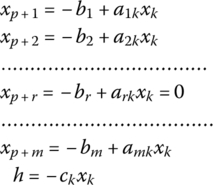
where x_p + 1, …, x_p + m are nonnegative slack variables. If the basic variables are taken to be those corresponding to the m + 1 unit column vectors in (6.6), then

(6.7)

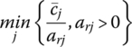
and thus our initial primal basic solution amounts to x_p + i =  − b_i, i = 1, …, m, and h = 0. Since this current solution is dual feasible (primal optimal) but not primal feasible, let us reduce primal infeasibility by choosing the vector to be removed from the basis according to

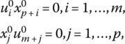
Hence, column p + r is deleted from the current basis so that x_p + r decreases in value to zero. By virtue of the weak complementary slackness conditions

it is evident that the dual variable u_r can increase in value from zero to a positive level. To determine the largest allowable increase in u_r that preserves dual feasibility, let us construct the simplex matrix associated with the dual problem as

(6.8)

wherein u_m + 1, …, u_m + p are nonnegative slack variables. From the m + 1 unit column vectors in (6.8) we have

(6.9)

Thus, an initial dual basic feasible solution consists of u_m + j = c_j, j = 1, …, p, and g = 0. If u_r is to enter the set of dual basic variables, (6.9) becomes

(6.9.1)

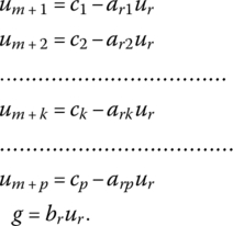
As u_r increases in value from zero, the new values of u_m + j, j = 1, …, p, must remain feasible, i.e. we require that

(6.9.2)

Under what conditions will this set of inequalities be satisfied? If a_rj ≤ 0, then u_m + j > 0 for any positive level of u_r, whence (6.9.1) indicates that g is unbounded from above and thus the primal problem is infeasible. Hence, we need only concern ourselves with those a_rj > 0. In this regard, when at least one of the coefficients a_rj within the rth row of (6.8) is positive, there exists an upper bound to an increase in u_r that will not violate (6.9.2). Rearranging (6.9.2) yields so that any increase in u_r that equals

preserves dual feasibility. Let us assume that, for j = k,

(6.10)

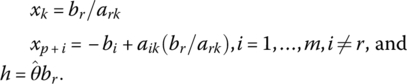
i.e. the dual basic variable u_m + k decreases in value to zero. But in terms of the preceding complementary slackness conditions, if u_m + k = 0, then x_k can increase to a positive level. Hence, from (6.6), column k replaces column p + r in the primal basis and thus x_k becomes a basic variable while x_p + r turns nonbasic. From (6.9.1), our new dual basic feasible solution becomes:

In terms of the primal problem, since

is equivalent to (6.10), x_k enters the set of primal basic variables and thus (6.7) simplifies to

or

As noted earlier, the dual simplex method is constructed so as to have its pivotal operations carried out within the standard primal simplex matrix. So from (6.6), if x_k is to replace x_p + r in the set of primal basic variables, a pivot operation with −a_rk as the pivotal element may be performed to express the new set of basic variables x_p + i, i = 1, …, m, i ≠ r, x_k, and h in terms of the nonbasic variables x₁, …, x_k − 1, x_k + 1, …, x_p, and x_p + r. To this end, (6.6) is transformed to

(6.11)

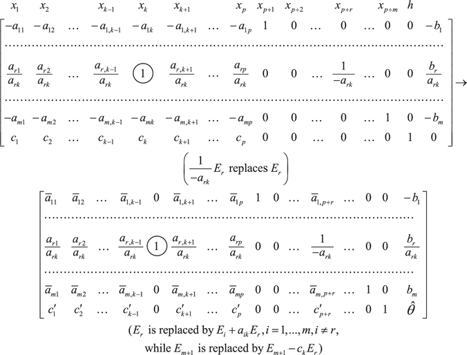
where

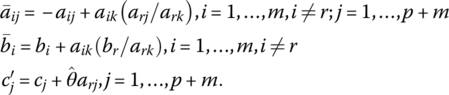
Hence our new primal basic solution is readily obtainable from (6.11) as

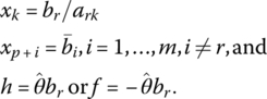
This pivotal process is continued until we obtain a basic feasible solution to the primal problem, in which case we have derived optimal basic feasible solutions to both the primal and dual problems.

6.7 Summary of the Dual Simplex Method

Let us now consolidate our discussion of the theory and major computational aspects of the dual simplex method. If we abstract from the possibility of degeneracy, then a summary of the principal steps leading to an optimal basic feasible solution to both the primal and dual problems simultaneously is:

1. Obtain an initial dual feasible (primal optimal) solution with
2. If primal feasibility also holds, then the current solution is an optimal basic feasible solution to both the primal and dual problems. If not all x_Bi ≥ 0, i = 1, …, m (primal feasibility is relaxed), then proceed with the next step.
3. Find 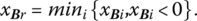The vector b_r corresponding to the minimum is to be removed from the basis.
4. Determine whether −a_rj ≥ 0, j = 1, …, m. If the answer is yes, the process is terminated since, in this instance, the primal problem is infeasible and thus the dual objective function is unbounded. If the answer is no, step 5 is warranted.
5. Compute 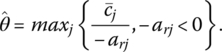If replaces b_r in the basis.

At this point, let us contrast the pivot operation involved in the dual simplex method with the one encountered previously in the primal simplex method. First, only negative elements can serve as pivotal elements in the dual simplex method whereas only positive pivotal elements are admitted in the primal simplex routine. Second, the dual simplex method first decides which vector is to leave the basis and next determines the vector to enter the basis. However, just the opposite order of operations for determining those vectors entering and leaving the basis holds for the primal simplex method.

2. Determine the new dual feasible (primal optimal) solution by pivoting on −a_rk. Return to step 2.

   By continuing this process of replacing a single vector in the basis at a time, we move to a new dual feasible solution with the value of the dual objective function diminished and primal infeasibility reduced. The process is terminated when we attain our first primal feasible solution, in which case we attain an optimal basic feasible solution to both the primal and dual problems.