14.1 Introduction

(Charnes et al. 1978; Banker et al. 1984; Seiford and Thrall 1990; and Banker and Thrall 1992)

In this chapter we shall examine an important applications area of linear programming, namely the technique of data envelopment analysis (DEA) that was first introduced by Charnes, Cooper, and Rhodes (1978). Generally speaking, DEA is a computational procedure used to estimate multiple‐input, multiple‐output production correspondences so that the productive efficiency of decision making units (DMUs) can be scrutinized. It accomplishes this by using linear programming modeling to measure the productive efficiency of a DMU relative to that of a set of baseline DMUs. In particular, linear programming is used to estimate what is called a best‐practice extremal frontier. It does so by constructing a piecewise linear surface, which essentially “rests on top” of the observations. This frontier “envelops” the data and enables us to determine a set of efficient projections to the envelopment surface. The nature of the projection path to the said surface depends on whether the linear program is input‐oriented or output‐oriented:

• Input‐oriented DEA – the linear program is formulated so as to determine the amount by which input usage of a DMU could be contracted in order to produce the same output levels as best practice DMUs.
• Output‐oriented DEA – the linear program is formulated so as to determine a DMU’s potential output given its inputs if it operated as efficiently as the best‐practice DMUs.

Moreover, the envelopment surface obtained depends on the scale assumptions made, e.g. we can posit either constant returns to scale (CRS) (output changes by the same proportion as the inputs change) or variable returns to scale (VRS) (the production technology can exhibit increasing, constant, or decreasing returns to scale).

Additional features of DEA models include the following:

1. They are nonparametric in that no specific functional form is imposed on the model, thus mitigating the chance of confounding the effects of misspecification of the functional form with those of inefficiency.
2. They are nonstochastic in that they make no accommodation for the effects of statistical noise on measuring the relative efficiency of a DMU.
3. They build on the individual firm efficiency measures of Farrell (1957) by extending the basic (engineering) ratio approach to efficiency measurement from a single‐output, single‐input efficiency index to multiple‐output, multiple‐input instances without requiring preassigned weights. This is accomplished by the extremal objective incorporated in the model, thus enabling the model to envelop the observations as tightly as possible.
4. They measure the efficiency of a DMU relative to all other DMUs under the restriction that all DMUs lie on or below the efficient or envelopment frontier.

Before we look to the construction of DEA models proper, some additional conceptual apparatus needs to be developed, namely: the set theoretic representation of a production technology, output, and input distance functions (IDFs), and various efficiency measures.

14.2 Set Theoretic Representation of a Production Technology

(Färe et al. 2008; Lovell 1994; Färe and Lovell 1978; and Fried et al. 2008)

Suppose x is an (n × 1) variable input vector in is an (m × 1) variable output vector in Then a multi‐input, multi‐output production technology can be described by the technology set

(14.1)

(T is also termed the production possibility set or the graph of the technology.) Clearly T contains all feasible correspondences of inputs x capable of producing output levels q. Moreover, the DMUs operate in T; and once T is determined, the location of a DMU within it enables us to gauge its relative efficiency and (local) returns to scale.

Looking to the properties of the technology set T(x, q) we note that: T is closed (it contains all of its boundary points); bounded (it has a finite diameter); and satisfies strong disposability, i.e. if (x, q) ∈ T, then (x₁, q₁) ∈ T for all (x₁, −q₁) ≥ (x, −q) or x₁ ≥ x and q₁ ≤ q.

The technology set T(x, q) contains its isoquants

(14.2)

(for (x, q) ∈ T, decreasing inputs by a fraction δ, 0 < δ < 1, does not allow us to increase outputs), which, in turn, contain efficient subsets

(14.3)

A multi‐input, multi‐output production technology can equivalently be represented by output and input correspondences derived from the technology set T. The output correspondence or output setP(x) is the set of all output vectors q that can be produced using the input vector x. Thus

(14.4)

Here P maps inputs x into subsets P(x) of outputs. In terms of the properties of P(x), for each x, P(x) satisfies:

1. 
2. Nonzero output levels cannot be produced from x = O.
3. P(x) is closed (P(x) contains all of its boundary points).
4. P(x) is bounded above (unlimited outputs cannot be produced from a given x).
5. P(x) is convex (i.e. if q₁and q₂ lie within P(x), then q^* = θq₁ + (1 − θ)q₂ ∈ P(x), 0 ≤ θ ≤ 1. So if q₁and q₂ can each be produced from a given x, then any internal average of these output vectors can also be produced).
6. P(x) satisfies strong (free) disposability of outputs (if q ∈ P(x) and q^* ≤ q, then q^* ∈ P(x)). Looked at in an alternative fashion, we can say that outputs are strongly disposable if they can be disposed of without resource use or cost.¹
7. P(x) satisfies strong disposability of inputs (if q can be produced from x, then q can be produced from any x^* ≥ x).

Output sets P(x) contain their output isoquants

(14.5)

which, in turn, contain their output efficient subsets

(14.6)

A moment’s reflection reveals that Eff P(x) ⊆ Isoq P(x) ⊆ P(x) (see Figure 14.1a). The output set P(x) is the area with the piecewise linear boundary OABCDEF, the output isoquant Isoq P(x) is ABCDEF, and the output efficient subset of the output isoquant is BCDE (it has no horizontal or vertical components).

The input correspondence or input set L(q) is the set of all input vectors x that can produce the output vector q. Hence

(14.7)

Looking to the properties of L(q), for each q, L(q) satisfies:

1. L(q) is closed (L(q) contains all of its boundary points).
2. L(q) is bounded below.
3. L(q) is convex (i.e. if x₁, x₂ ∈ L(q), then x^* = θx₁ + (1 − θ)x₂ ∈ L(q), 0 ≤ θ ≤ 1).
4. L(q) satisfies strong disposability of inputs (if x ∈ L(q) and if x^* ≥ x, then x^* ∈ L(q)).

   (Inputs are weakly disposable if x ∈ L(q) implies that, for all λ ≥ 1, λx ∈ L(q).)

Input sets L(q) contain their input isoquants

(14.8)

which, in turn, contain their input efficient subsets

(14.9)

Given these constructs, it is readily seen that Eff L(q) ⊆ Isoq L(q) ⊆ L(q) (Figure 14.1b). The input set L(q) is the area to the right and above the piecewise linear boundary ABCDE, the input isoquant Isoq L(q) is ABCDE, and the input efficient subset of the input isoquant is BCD (it has no horizontal or vertical elements).

On the basis of the preceding discussion, we can redefine the output set P(x) (Eq. (14.4)) and input set L(q) (Eq. (14.7)) as

(14.4.1)

and

(14.7.1)

respectively. This enables us to obtain the input and output correspondences from one another since if q ∈ P(x), then x ∈ L(q). Hence P(x) and L(q), being inversely related, contain the same information.

14.3 Output and Input Distance Functions

(Färe and Lovell 1978; Fried et al. 2008; Coelli et al. 2005; and Shephard 1953, 1970)

Output and input distance functions serve as an alternative way of describing a multi‐output, multi‐input technology. Moreover, as we shall see in the next section, such functions will be utilized to measure the efficiency of a DMU in production.

We start with the output distance function (ODF) – considers a maximal proportional expansion of the output vector q, given an input vector x. The ODF is defined on the output set P(x) as

(14.10)

(assuming that the minimum is actually attained).

To evaluate (14.10), let us see how δ is determined. Looking to Figure 14.2a, suppose δ^* = min {δ|(q/δ) ∈ P(x)}, q is located at point A, with (q/δ^*) found at point B. Then the ODF at Point A is δ^* = OA/OB < 1 so that (q/δ^*) lies on Isoq P(x). By definition, δ^* is the smallest δ that puts (q/δ^*) on the boundary of P(x). (Clearly the value of the ODF at points B and C is 1.)

Key properties of the ODF are:

1. 
2. d₀(x, q) is nonincreasing in x and nondecreasing in q.
3. d₀(x, q) is linearly homogeneous (or homogeneous of degree 1) in q.²
4. if q ∈ P(x), then d₀(x, q) ≤ 1.
5. if q ∈ Isoq P(x), then d₀(x, q) = 1.
6. d₀(x, q) is quasi‐convex³ in x and convex⁴ in q.

We next examine the input distance function (IDF). Specifically, the IDF characterizes a production technology by specifying the minimal proportional contraction of the input vector x, given the output vector q. In this regard, the IDF can be expressed as

(14.11)

(It is assumed that the maximum is realized.)

How is ρ to be determined? In Figure 14.2b, let ρ^* = max {ρ|(x/ρ) ∈ L(q)} with x found at point A and (x/ρ^*) located at point B. Then the IDF at point A is ρ^* = OA/OB > 1 so that (x, ρ^*) lies on Isoq L(q). By definition, ρ^* is the largest ρ which puts (x/ρ^*) on the boundary of L(q). (Note that the IDF at points B and C is 1.)

Properties of the IDF are:

1. d_I(x, q) is nondecreasing in x and nonincreasing in q.
2. d_I(x, q) is linearly homogeneous (or homogeneous of degree 1) in x.
3. If x ∈ L(q), then d_I(x, q) ≥ 1.
4. If x ∈ Isoq L(q), then d_I(x, q) = 1.
5. d_I(x, q) is concave⁵ in x and quasi‐concave⁶ in q.

What is the connection between the output and IDFs? It should be evident that if q ∈ P(x), then x ∈ L(q). Moreover, if inputs and outputs are weakly disposable, then it can be shown that d₀(x, q) ≤ 1 if and only if d_I(x, q) ≥ 1. And if the technology is subject to CRS, then d₀(x, q) = 1/d_I(x, q) for all x, q.

14.4 Technical and Allocative Efficiency

As indicated above, the principal focus of DEA is the assessment of the relative efficiency of a DMU. Generally speaking, the efficiency of a DMU consists of two components: technical and allocative. Specifically, technical efficiency (TE) can have an input‐conserving orientation or an output‐augmenting orientation, i.e.

1. Input‐conserving orientation – given the technology and output vector q, the DMU utilizes as little of the inputs x as possible;
2. Output‐augmenting orientation – given the technology and input vector x, the DMU maximizes the outputs q produced.⁷(14.12)

Next, allocative efficiency (AE) refers to the use of inputs in optimal proportions given their market prices and the production technology. In what follows, we shall develop in greater detail the notion of technical and AE (see Sections 14.4.1 and 14.4.2, respectively).

14.4.1 Measuring Technical Efficiency

(Debreu 1951; Farrell 1957)

Let us assume that the production process exhibits CRS. In two dimensions, TE will be measured along a ray from the origin to the observed production point. (This obviously holds the relative proportions of inputs constant.) In this regard, the measures or indexes of TE that follow are termed radial measures of TE. Given this convention, we may modify our definitions of input‐oriented and output‐oriented TE (14.12a, b) to read:

1. Input‐conserving orientation – we are interested in determining the amount by which input quantities can be proportionately reduced without changing the output quantities produced.
2. Output‐augmenting orientation – we are interested in determining the amount by which output quantities can be proportionately increased without changing the input quantities used.(14.13)

Let us first examine the input‐oriented case. Suppose that a DMU uses two inputs to produce a single output. If the production function appears as q = f(x₁,x₂), then, under CRS, k = 1 in footnote 1. Set so that Hence, the technology can be represented by the unit isoquant. In this regard, let the unit isoquant of fully efficient DMUs be depicted as II′ in Figure 14.3. Suppose P represents the observed input combination x that produces a unit of output. Then the (absolute) technical inefficiency of the DMU is represented by the distance QP – the amount by which all inputs could be proportionately reduced without a reduction in output so that QP/OP is the percentage by which all inputs need to be reduced to attain production efficiency. Since QP = OP−OQ, set

(14.14)

so that we can measure the degree of input‐oriented TE of a DMU as

(14.15)

Here, TE_I depicts the ratio of inputs needed to produce q to the inputs actually used to produce q, given x. (Note: if TE_I = 1, then a DMU is fully efficient since its input combination lies on the unit isoquant II′, e.g. point Q in Figure 14.3.) Point Q is therefore point P’s technically efficient projection point on the unit isoquant. More formally, we can state the input‐oriented measure of TE (Debreu 1951; Farrell 1957). A radial measure of the TE of input vector x in the production of output vector q is

(14.16)

So for x ∈ L(q), TE_I(x, q) ≤ 1. Hence θ = 1 indicates radial TE (x ∈ Isoq L(q)) and θ < 1 indicates the degree of radial technical inefficiency.

(In Figure 14.3, let θ = 1 − QP/OP. Then θP puts us at point Q on the unit isoquant.) A moment’s reflection reveals that: (i) Eff L(q) ⊆ Isoq L(q) = {x|TE_I(x, q) = 1}; and (ii) TE_I(x, q) = 1/d_I(x, q). (For a fully efficient DMU, TE_I(x, q) = 1 = d_I(x, q).)

Second, we turn our attention to the output‐oriented case. Let us assume that a DMU produces two outputs (q₁ and q₂) from a single input x. If the production possibility curve can be written as x = g(q₁, q₂), then, under CRS, we can obtain g(q₁/x, q₂/x, ) = 1. Hence, the technology can be represented by the unit production possibility curve and thus the unit production possibility curve of fully efficient DMUs can be denoted PP′ in Figure 14.4. Let point A represent the observed output combination that utilizes 1 unit of x. Then the (absolute) technical inefficiency of the DMU is depicted by the distance AB – the amount by which output could be proportionately increased without requiring more input so that AB/OA is the percent by which all outputs could be increased to attain production efficiency. Given that AB = OB − OA, set

(14.17)

so that we can measure the degree of output‐oriented TE of a DMU as

(14.18)

It is instructive to note that, whether measuring input‐oriented or output‐oriented TE, we are always forming the ratio between the optimal production point and the actual production point, e.g. see TE_I = OQ/OP (Figure 14.3) and TE₀ = OB/OA(Figure 14.4). We may view TE₀ as indicating the ratio of outputs efficiently produced by x to the outputs actually produced by x, given q. (Note: if TE₀ = 1, then a DMU is fully efficient since its output combination lies on the unit production possibility curve PP′, i.e. point B in Figure 14.4.) Point B is thus A’s technically efficient projection point on the unit production possibility curve. In this regard we can now state that output‐oriented measure of TE (Debreu 1951; Farrell 1957). A radial measure of the TE of output vector q produced by input vector x is

(14.19)

So for q ∈ P(x), TE₀(x, q) ≥ 1. That is, ϕ = 1 indicates radial TE (q ∈ Isoq P(x)) and ϕ > 1 indicates the degree of radial technical inefficiency.

(In Figure 14.4, let ϕ = 1 + AB/OA. Then ϕA puts us at point B on the unit production possibility curve.) It is also true that: (i) Eff P(x) ⊆ Isoq P(x) = {q|TE₀(x, q) = 1}; and (ii) TE₀(x, q) = 1/d₀(x, q). (For a fully efficient DMU, TE₀ (x, q) = 1 = d₀(x, q).)

14.4.2 Allocative, Cost, and Revenue Efficiency

(Lovell 1994; Coelli et al. 2005)

Suppose a DMU uses the inputs (x₁ and x₂) to produce a single output (q) under CRS. (The unit isoquant of fully efficient firms is again denoted II′ in Figure 14.5.) Moreover, if the input prices (w₁ and w₂) are known and assumed fixed, then the isocost line AA′ with slope −w₁/w₂ can also be plotted in Figure 14.5. Here P depicts the actual production point with input vector x; Q is P’s technically efficient projection point with input vector x; and S denotes the cost‐minimizing point with input vector x^*. Given the isocost line AA′, we know that AE involves the selection of an input mix that assigns factors of production to their optimal or best alternative uses based upon their opportunity costs. Clearly point S minimizes the cost of producing the single unit of output depicted by II′. Since the cost at R is the same as that of the allocatively efficient point S, and is less than that incurred at the technically efficient point Q, we can measure AE as AE = OR/OQ.⁸ In addition, since RQ represents the reduction in production cost that would occur if production were carried out at S instead of Q, then, under a parallel shift of the isocost line AA′ to BB′, RQ/OQ depicts the proportionate reduction in cost associated with a movement from Q to S.

		P	Q	S
Efficiency	Technically efficient	No	Yes	Yes
Status	Allocatively efficient	No	No	Yes

Since TE and AE are measured along the same ray from the origin to the inefficient point P, the inefficient input proportions are held constant so that the efficiency measures TE and AE must be independent. In this regard, given TE = OQ/OP, the overall cost efficiency (CE) of the DMU can be expressed as the composite index

(14.20)

(Note: CE ≤ TE; and CE ≤ 1/d_I(x, q).)

It should be evident that AE and CE are input‐oriented concepts. We now turn to an output‐oriented measure of efficiency, namely revenue efficiency (RE). To this end, let the outputs q₁ and q₂ be produced by the single fixed input x under CRS. Then the unit production possibility curve of fully efficient DMUs can be represented as PP′ in Figure 14.6. Additionally, if the output prices (p₁and p₂) are observed and assumed fixed, then the isorevenue line EE′ with slope −p₁/p₂ can also be plotted in Figure 14.6. Here A depicts the actual output point with output vector q; B represents A’s technically efficient projection point with output vector ; and D denotes the revenue maximizing point with output vector q^*.⁹

		A	B	D
Efficiency	Technically efficient	No	Yes	Yes
Status	Allocatively efficient	No	No	Yes

Let us express the TE of output point A as TE = OA/OB while the AE of the DMU can be determined as AE = OB/OC. Then the overall RE of the DMU is

(14.21)

(Note: RE ≤ TE; and RE ≥ 1/d₀(x, q).)

14.5 Data Envelopment Analysis (DEA) Modeling

(Charnes et al. 1978; Cooper et al. 2007; Lovell 1994; Banker et al. 1984; Banker and Thrall 1992)

In the models that follow, we shall employ linear programming techniques to construct a nonparametric, piecewise linear surface (or frontier) to cover or envelop the data points. Efficiency measures are then determined relative to this surface. Suppose we have N inputs, M outputs, and I DMUs. Then to calculate these efficiency measures, a set of input weights w_r, r = 1, …, N, and output weights u_s, s = 1, …, M, will be derived from the data and not taken in advance to be fixed. As will be noted below, a group of DMUs is used to evaluate each other, with each DMU displaying various degrees of managerial freedom in pursuing its individual goals.

For the jth DMU, the input and output vectors are, respectively,

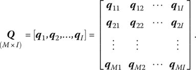
where x_rj is the amount of the rth input used by DMU_j and q_sj is the amount of the sth output produced by the DMU_j. (All components of these input and output vectors are assumed to be nonnegative, with at least one component within each taken to be positive. Thus x_j, q_j are semi‐positive, i.e. x_j ≥ 0 and x_j ≠ 0; q_j ≥ 0 and q_j ≠ 0.) Then the (N × I) input matrix X can be written as

and the (M × I) output matrix Q can be expressed as

Next, let the (N × 1) vector of input weights and the (M × 1) vector of output weights be denoted, respectively, as

14.6 The Production Correspondence

We noted earlier that DMU_j has at least one positive value in both the input and output vectors x_j ∈ R^N and q_j ∈ R^M, respectively. Let us refer to each pair of semi‐positive input and output vectors (x_j, q_j) as an activity. The set of feasible activities is termed the production possibility setR with these properties:

1. Observed activities (x_j, q_j), j = 1, …, I, belong to R.
2. If an activity (x, q) ∈ R, then (tx, tq) ∈ R for t, a positive real scalar (the CRS assumption).
3. If activity (x, q) ∈ R, then any semi‐positive activity with 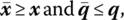belongs to R.
4. Any semi‐positive linear combination of observed activities belongs to R (i.e. R is a convex set).

Under these properties, if we observe I DMUs with activities (x_j, q_j), j = 1, …, I, then, given the input and output matrices X and Q, respectively, and a semi‐positive vector λ ∈ R^I, we can define the production possibility set as

Looking to the structure of R we see that for the activity (x, q), x ≥ Xλ (think of Xλ as the input vector of the combined activities) or

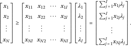
Here, represents the sum of weighted inputs that cannot exceed x_r, r = 1, …, N. Also, q ≤ Qλ (we may view Qλ as the output vector of the combined activities) or

Thus, depicts the sum of weighted outputs which cannot fall short of q_s, s = 1, …, M. These inequalities stipulate that R cannot contain activities (x, q) which are more efficient than linear combinations of observed activities.

14.7 Input‐Oriented DEA Model under CRS

(Charnes et al. 1978)

Given the set of input and output observations, let us define the total factor productivity of a given DMU, say DMU_o, as

(14.22)

where U′q_o is a (virtual) measure of aggregate output produced and W′x_o is a (virtual) measure of aggregate input used. Given (14.22), we can form the following fractional program so as to obtain the input and output weights w_r, r = 1, …, N, and u_s, s = 1, …, M, respectively. Since these weights are the unknowns or variables, the said program is structured as

(14.23)

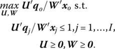
Clearly this problem involves finding the values of the input and output weights such that the total factor productivity (our efficiency measure) of DMU_o is maximized subject to the normalizing constraints that all efficiency measures must be less than or equal to unity. Since j = 1, …, I, we need I separate optimizations, one for each DMU to be evaluated, where the particular DMU under consideration receives the “o” designation. Hence each DMU is assigned its own set of optimal input and output weights.

Given that the fractional program (14.23) is nonlinear, it can be converted to a linear program in multiplier form via the following change of variables (see CCR 1978) from W, U to ν, μ. That is, for μ = tU, ν = tW and t = (W′x_o)⁻¹, set in (14.23) so as to obtain

(14.23.1)

Since 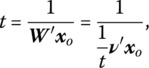it follows that ν′x_o = 1. Hence (14.23.1) can ultimately be rewritten as

(14.23.2)

the multiplier form of the DEA input‐oriented problem. Here (14.23.2) involves M + N variables in I + 1 structural constraints.

We note briefly that: (i) the fractional program (14.23.1) is equivalent to the linear program (14.23.2); and (ii) the optimal objective function values in (14.23.1) and (14.23.2) are independent of the units in which the inputs and outputs are measured (given that each DMU uses the same units of measurement). Hence our measures of efficiency are units invariant.

The optimal solution to (14.23.2) will be denoted as λ^*, μ^*, and ν^*, where μ^*and ν^* represent optimal price vectors. Given this solution, let us consider the concept of CCR‐efficiency. Specifically, CCR‐efficiency: (i) DMU_o is CCR‐efficient if γ^* = 1 and there exists at least one optimal set of price vectors (μ^*, ν^*) with μ^* > 0, ν^* > 0; and (ii) otherwise DMU_o is CCR‐inefficient.

Hence DMU_o is CCR‐inefficient if either (i) γ^* < 1 or (ii) γ^* = 1 and at least one element of (μ^*, ν^*) is zero for every optimal solution to (PLP_o). Suppose DMU_o is CCR‐inefficient with γ^* < 1. Then there must be at least one DMU whose constraint in (μ^*)′Q − (ν^*)′X ≤ 0′ holds as a strict equality since, otherwise, γ^* is suboptimal. Let the set of such j ∈ J = {1, …, I} be denoted as

Let the subset be composed of CCR‐efficient DMUs. It will be termed DMU_o’s reference set or peer group. Clearly, it is the existence of this collection of efficient DMUs that renders DMU_o inefficient. The set spanned by E_o is DMU_o’s efficient frontier. Thus, all inefficient DMUs are measured relative to their individual reference sets.

The dual of the multiplier problem (14.23.2) is termed the input‐oriented envelopment form of the DEA problem and appears as

(14.24)

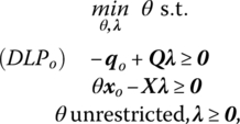
where θ is a real dual variable and λ is an I + 1 vector of nonnegative dual variables. Here (14.24) involves I + 1 variables and M + N constraints.

Let us examine the structure of (PLP_o) and (DLP_o) in greater detail. Looking to their objectives:

• (PLP_o) – seeks to determine the vectors of input and output multipliers (or normalized shadow prices) that will maximize the value of output q_o.
• (DLP_o) – seeks to determine a vector λ that combines the observed activities of the I firms and a scalar θ that depicts the level of input contraction required to adopt a technically efficient production technology. In this regard, θ(≤1) will be termed the efficiency score for the jth DMU. And if θ = 1, then the DMU is on the frontier and consequently is termed technically efficient. As indicated earlier, this program must be solved I times (once for each DMU).

Additionally, the usual complementarity between primal variables and dual structural constraints and between dual variables and primal structural constrains holds (see Table 14.3).

Due to the nonzero restriction on the input and output data, the dual constraint −q_o + Qλ ≥ 0 requires that λ ≠ 0 since q_o ≥ 0 and q_o ≠ 0. Thus, from θx_o − Xλ ≥ 0, we have θ > 0 so that the optimal value of θ, θ^* must satisfy 0 < θ^* ≤ 1. Moreover, from linear programming duality (Theorem 6.2), μ′q_o ≤ θ at a feasible solution and, at the optimum, (μ^*)′q_o = θ^* ≤ 1. Clearly input‐oriented radial efficiency requires (μ^*)′q_o = θ^* = 1.

What is the connection between the production possibility set R and the dual problem (DLP_o)? The constraints of (DLP_o) restrict the activity (θx_o, q_o) to R while the objective in (DLP_o) seeks the θ that produces the smallest (radial) contraction of the input vector x_o while remaining in R. Hence, we are looking for an activity in R that produces at least q_o of DMU_o while shrinking x_o proportionately to its smallest feasible level.

14.8 Input and Output Slack Variables

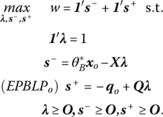
When θ^* < 1, the proportionately reduced input vector θ^*x_o indicates the fraction of x_o that is needed to produce q_o efficiently, with (1 − θ^*) serving as the maximal proportional reduction allowed by the production possibility set if input proportions are to be kept invariant. Hence input excesses and output shortfalls can obviously exist. In this regard, from (DLP_o), let us define the slack variables s⁻ ∈ R^N and s⁺ ∈ R^M, respectively, as wasted inputss⁻ = θx_o − Xλ ≥ 0 and forgone outputss⁺ =  − q_o + Qλ ≥ 0. To determine any input excesses or output shortfalls, let us employ the following two‐phase approach:

• Phase I. Solve (DLP_o) in order to obtain θ^*. (Remember that, at optimality, θ^* equals the (PLP_o) objective value and that serves as the Farrell efficient or CCR‐efficient value.)
• Phase II Extension of (DLP_o). Given θ^*, determine the optimal λ that maximizes the input slacks s⁻ = θ^*x_o − Xλ and output slacks s⁺ = Qλ − q_o. Given that λ, s⁻, and s⁺ are all variables, this Phase II linear program is

(14.25)

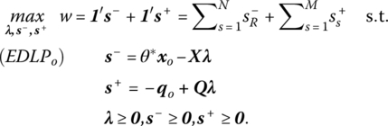
Clearly, this Phase II problem seeks a solution that maximizes the input excesses and output shortfalls while restricting θ to its Phase I value θ^*.

A couple of related points concerning this two‐phase scheme merit our attention. First, an optimal solution (λ^*, (S⁻)^*, (S⁺)^*) to (14.25) is called a maximal‐slack solution. If any such solution has (S⁻)^*  = O^N and (S⁺)^*  = O^M, then it is termed a zero‐slack solution. Second, if an optimal solution (θ^*, λ⁺, (S⁻)^*, (S⁺)^*) to the two‐phase routine has θ^* = 1 (it is radially efficient) and is zero‐slack, then DMU_o is CCR‐efficient. Thus, DMU_o is CCR‐efficient if no radial contraction in the input vector x_o is possible and there are no positive slacks. Relative to some of our preceding efficiency concepts, we note briefly that:

1. if θ^* = 1 with (S⁻)^*  ≥ 0 or (S⁺)^*  ≥ 0, then DMU_o is Farrell efficient; but
2. if θ^* = 1 and (S⁻)^*  = O^N, (S⁺)^*  = O^M, then DMU_o is Koopmans efficient.

14.9 Modeling VRS

(BCC 1984; Cooper et al. 2007; Banker and Thrall 1992 and Banker et al. 1996)

14.9.1 The Basic BCC (1984) DEA Model

The CCR (1978) DEA model considered earlier was specified under the assumption of CRS. We may modify the CCR (1978) model to accommodate the presence of VRS by looking to the DEA formulation offered by BCC (1984).

To introduce VRS, BCC (1984) add 1′λ = 1 to the constraint system in the envelopment form of the input‐oriented DEA problem. This additional constraint (called the convexification constraint) admits only convex combinations of DMUs when the efficient production frontier is formed. This convexification constraint essentially shrinks the production possibility set T to a new production possibility set (so that ) and thus converts a CRS technology to a VRS technology, where the letter production possibility set has the form

This revised technology set satisfies strong disposability and convexity but not homogeneity; it amounts to a polyhedral convex free disposal hull. In fact, it is the smallest set satisfying the convexity and strong disposability property subject to the condition that each activity (x_j, q_j), j = 1, ⋯, I, belongs to . As we shall see below, the convexification constraint leads to the definition of a new variable that determines whether production is carried out in regions of increasing, decreasing, or CRS. Hence, we shall examine returns to scale locally at a point on the efficiency frontier, and ultimately relate it to the sign of this new variable.

The input‐oriented BCC (1984) model is designed to evaluate the efficiency of DMU₀ by generating a solution to the envelopment form of the (primal) linear program

(14.26)

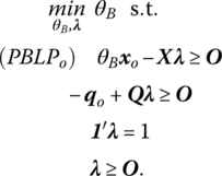
The dual to (PBLP_o) is its multiplier form

(14.27)

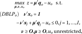
where u_o is the dual variable associated with the convexification constraint 1′λ = 1 in (14.26).¹⁰

It is instructive to examine the geometric nature of an optimal solution to the dual problem (DBLP_o). If the I constraint inequalities in (14.27) are replaced by −v′X + μ′Q − u_o1 ≤ O, then we can interpret this inequality as a supporting hyperplane to at the optimum. In this regard, the vector of coefficients (v^*, μ^*, u_o^*) of the supporting hyperplane to is an optimal solution to the dual problem (14.27).

14.9.2 Solving the BCC (1984) Model

Let us focus on the envelopment form (PBLP_o). A solution to this problem can be obtained by employing a two‐phase routine similar to that used to solve the CCR dual program (DBLP_o), i.e.

• Phase I. Solve (PBLP_o) in order to obtain
• Phase II Extension of (PBLP_o). Given , determine the optimal λ which maximizes the input slacks s⁻ and the output slacks s⁺. Thus, the Phase II linear program is

(14.29)

Let an optimal solution to (14.29) be denoted as An important characterization of this solution is provided by the notion of BCC‐Efficiency: (i) If program (EPBLP_o) generates an optimal solution for (PBLP_o) with and (s⁻)^* = O^N, (s⁺)^* = O^M, then DMU_o is termed BCC‐efficient; (ii) otherwise, it is called BCC‐inefficient.

Moreover, if DMU_o is BCC‐efficient, its reference setE_o can be expressed as

Given the possibility of multiple optimal solutions to (14.29), any one of them may be selected to determine

(14.30)

so that an improved activity can be calculated (via the BCC‐projection) as

(14.31)

In addition, it can be demonstrated that this improved activity is BCC‐efficient (on all this see Cooper et al. 2007).

14.9.3 BCC (1984) Returns to Scale

We noted in the preceding section that u_o is a dual variable associated with the convexification constraint 1′λ = 1 in (14.26). It was also mentioned that the constraint −v′X + μ′Q − u_o1 ≤ O in the dual problem (DBLP_o) is a supporting hyperplane to at an optimal solution (ν^*, μ^*, u_o^*). Thus, (ν^*, μ^*, u_o^*) is an optimal solution to the dual problem (DBLP_o) associated with the primal problem (PBLP_o). So if DMU_o is BCC‐efficient, the vector of coefficients (ν^*, μ^*, u_o^*) of the supporting hyperplane to at (x_o, q_o) renders an optimal solution to (PBLP_o), and vice versa. So, when a DMU is BCC‐efficient, we can rely on the sign of to describe returns to scale (specifically, returns to scale as described in Banker and Thrall (1992)). Given that (x_o, q_o) is on the efficient frontier:

1. Increasing returns to scale exist at (x_o, q_o) if and only if for all optimal solutions.
2. Decreasing returns to scale exist at (x_o, q_o) if and only if for all optimal solutions.
3. Constant returns to scale exist at (x_o, q_o) if and only if in any optimal solution.

It is instructive to examine a simplified application of (i)–(iii). Let us consider the single‐input, single‐output case (Figure 14.8). In this instance, the supporting hyperplane to has the form −vx + uq = u_o. Additionally, we know that the average product AP = q/x is calculated as the slope of a ray from the origin to the VRS frontier. Clearly, AP is increasing as x increases from 0 to x_o (e.g. see the plane of support which is tangent to along edge AB). AP reaches a maximum at Point B (when x = x_o with u_o = 0) and then begins to decrease as x is increased beyond x_o (e.g. is tangent to along edge BC). Hence we have a range of increasing returns from 0 to x_o (with ), constant returns at x_o (where u_o = 0), and a range of decreasing returns beyond x_o (with ).

Suppose we have obtained an optimal solution to the (PBLP_o) envelopment problem (14.26). Then we may project (x_o, q_o) into a point on the efficient frontier using the BCC‐projection

(14.32)

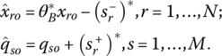
Additional details on the use of (14.32) in forming a modified dual (multiplier) problem can be found in Banker et al. (1996) and in Cooper et al. (2007).

14.10 Output‐Oriented DEA Models

We noted at the outset of this chapter that, in general, an input‐oriented DEA model focuses on the minimization of input usage while producing at least the observed output level. That is, it identifies TE as the proportionate reduction in input usage, with output levels kept constant. In contrast to this modeling approach, an output‐oriented DEA model maximizes output while using no more than the observed inputs. Now TE is measured as the proportionate increase in output, with input levels held fixed. These two efficiency measures are equivalent or render the same objective function value under CRS but display unequal objective values when VRS is assumed.

Let us first consider the output‐oriented DEA model under CRS. It is structured in envelopment form as

(14.33)

As one might have anticipated, there exists a direct correspondence between the input‐oriented model (14.24) and the output‐oriented model (14.33). That is, the solution to (14.33) can be derived directly from the solution to (14.24). To see this, let

(14.34)

Then substituting (14.34) into (14.24) results in the output‐oriented model (14.33). So at optimal solutions to problems (14.33) and (14.24),

(14.34.1)

Since θ^* ≤ 1, it follows that η^* ≥ 1, i.e. as η^* increases in value, the efficiency of DMU_o concomitantly decreases. And while θ^* represents the input reduction rate, η^* depicts the output expansion rate, where η^* − 1 represents the proportionate increase in outputs that is achievable by DMU_o given that input levels are held constant. The TE for DMU_o is given by So if DMU_o is efficient in terms of its input‐oriented model, then it must also be efficient in terms of its associated output‐oriented model. Thus, the solution of the output‐oriented model (14.33) can be obtained from the solution to the input‐oriented model (14.24). In fact, the improvement in (x_o, q_o) can be obtained from

(14.35)

where t⁻ = x_o − Xμ and t⁺ = Qμ − ηq_o are the vectors of slack variables for (14.33). Additionally, at optimal solutions to problems (14.33) and (14.24),

(14.36)

Moreover, both the input‐ and output‐oriented DEA models will determine exactly the same efficient frontier, and thus label the same set of DMUs as efficient.

The dual of (14.33) is the output‐oriented multiplier problem

(14.37)

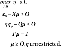
If we impose the assumption of VRS, then the appropriate output‐oriented DEA model (in envelopment form) appears as

(14.38)

Then the dual (multiplier) form of (14.38) is

(14.39)

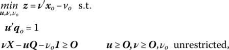
where v_o is the scalar associated with 1′μ = 1 in the envelopment form (14.38).