8
Sensitivity Analysis
8.1 Introduction
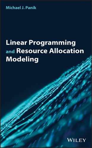
Throughout this chapter we shall invoke the assumption that we have already obtained an optimal basic feasible solution to a linear programming problem in standard form, i.e. to a problem of the form
We then seek to employ the information contained within the optimal simplex matrix to gain some insight into the solution of a variety of linear programming problems that are essentially slight modifications of the original one. Specifically, we shall undertake a sensitivity analysis of the initial linear programming problem, i.e. this sort of post‐optimality analysis involves the introduction of discrete changes in any of the components of the matrices ![]() , in which case the values of cj, bi, or aij, i = 1, …, m; j = 1, …, n − m, respectively, are altered (increased or decreased) in order to determine the extent to which the original problem may be modified without violating the feasibility or optimality of the original solution. (It must be remembered, however, that any change in, say, the objective function coefficient ck is a ceteris paribus change, e.g. all other cj’s are held constant. This type of change also holds for the components of
, in which case the values of cj, bi, or aij, i = 1, …, m; j = 1, …, n − m, respectively, are altered (increased or decreased) in order to determine the extent to which the original problem may be modified without violating the feasibility or optimality of the original solution. (It must be remembered, however, that any change in, say, the objective function coefficient ck is a ceteris paribus change, e.g. all other cj’s are held constant. This type of change also holds for the components of ![]() )
)
8.2 Sensitivity Analysis
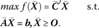
Turning again to our linear programming problem in standard form, let us
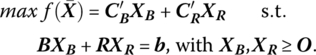
Then, as previously determined, with
It follows that if XR = O, the resulting solution is basic (primal) feasible if XB = B−1b ≥ O and optimal (dual feasible) if ![]()
8.2.1 Changing an Objective Function Coefficient
If we now change ![]() to
to ![]() then
then

Since XB = B−1b is independent of ![]() this new basic solution remains primal feasible while, if
this new basic solution remains primal feasible while, if ![]() dual feasibility or primal optimality holds. Since our discussion from this point on will be framed in terms of examining selected components within the optimal simplex matrix, it is evident from the last row of the same that primal optimality or dual feasibility is preserved if
dual feasibility or primal optimality holds. Since our discussion from this point on will be framed in terms of examining selected components within the optimal simplex matrix, it is evident from the last row of the same that primal optimality or dual feasibility is preserved if ![]() Let us now consider the various subcases that may obtain.
Let us now consider the various subcases that may obtain.
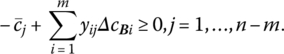
If ΔCB = O (so that an objective function coefficient associated with a nonbasic variable changes), it follows that optimality is preserved if ![]() i.e. if
i.e. if
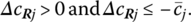
How may changes in cRj affect (8.1)? First, if cRj decreases in value so that ΔcRj < 0, then (8.1) is still satisfied. In fact, cRj may decrease without bound and still not violate (8.1). Hence the lower limit to any decrease in cRj is −∞. Next, if cRj increases so that ΔcRj > 0, then (8.1) will hold so long as cRj increases by no more than ![]() . Hence the only circumstance in which xRj becomes basic is if its objective function coefficient cRj increases by more than
. Hence the only circumstance in which xRj becomes basic is if its objective function coefficient cRj increases by more than ![]() . If
. If ![]() where
where ![]() is the new level of cRj, then the upper limit on
is the new level of cRj, then the upper limit on ![]() to which cRj can increase without violating primal optimality is
to which cRj can increase without violating primal optimality is ![]() .
.
If ΔCR = O (so that an objective function coefficient associated with a basic variable changes), it follows that the optimality criterion is not violated if ![]() i.e. if
i.e. if
Let us assume that cBk changes. Hence (8.2) becomes
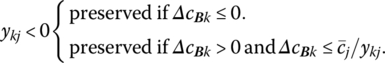
We now consider the circumstances under which changes in cBk preserve the sense of this inequality. First, if ykj = 0, then (8.2.1) holds regardless of the direction or magnitude of the change in cBk. Second, if ykj > 0, then (8.2.1) is satisfied if ΔcBk ≥ 0, i.e. ΔcBk may increase without bound. Hence, (8.2.1) is affected only when cBk decreases or ΔcBk < 0. Since (8.2.1) implies that ![]() it is evident that the lower limit to which ΔcBk can decrease without violating optimality is
it is evident that the lower limit to which ΔcBk can decrease without violating optimality is ![]() Hence, xRj remains nonbasic as long as its objective function coefficient does not decrease by more than
Hence, xRj remains nonbasic as long as its objective function coefficient does not decrease by more than ![]() Now, it may be the case that ykj > 0 for two or more nonbasic variables. To ensure that (8.2.1) is satisfied for all such j, the lower limit to which ΔcBk can decrease without violating the optimality of the current solution is
Now, it may be the case that ykj > 0 for two or more nonbasic variables. To ensure that (8.2.1) is satisfied for all such j, the lower limit to which ΔcBk can decrease without violating the optimality of the current solution is
Finally, if ykj < 0, (8.2.1) holds if ΔcBk ≤ 0, i.e. ΔcBk may decrease without bound without affecting primal optimality. Thus, the optimality criterion is affected by changes in cBk only when ΔcBk > 0. In this instance (8.2.1) may be written as ![]() so that the upper limit to any change in cBk is
so that the upper limit to any change in cBk is ![]() Hence xRj maintains its nonbasic status provided that the increase in cBk does not exceed
Hence xRj maintains its nonbasic status provided that the increase in cBk does not exceed ![]() . If ykj < 0 for two or more nonbasic variables, then (8.2.1) holds for all relevant j if the upper limit to which ΔcBk can increase is specified as
. If ykj < 0 for two or more nonbasic variables, then (8.2.1) holds for all relevant j if the upper limit to which ΔcBk can increase is specified as
Actually, the optimality criterion (8.2.1) will be maintained if both the lower and upper limits (8.3), (8.4), respectively, are subsumed under the inequality
Hence (8.5) provides the bounds within which ΔcBk may decrease or increase without affecting the optimality of the current solution. As an alternative to the approach pursued by defining (8.3), (8.4), we may express these limits in terms of the new level of cBk, call it ![]() , by noting that, for
, by noting that, for ![]() (8.3) becomes
(8.3) becomes
while (8.4) may be rewritten as
Hence (8.3.1) (8.4.1) specifies the lower (upper) limit to which cBk can decrease (increase) without violating the optimality criterion (8.2.1). In view of this modification, (8.5) appears as
One final point is in order. If cBk changes in a fashion such that (8.5) and (8.5.1) are satisfied, then the current basic feasible solution remains optimal but the value of the objective function changes to ![]()
Table 8.1 Limits to which cR1, cR2, and cR3 can increase or decrease without violating primal optimality.
| Nonbasic variables | Objective function coefficients | Lower limit | Upper limit |
| xR1 = x1 | cR1 = c1 = 2 | −∞ |
|
| xR2 = x4 | cR2 = c4 = 0 | −∞ |
|
| xR3 = x5 | cR3 = c5 = 0 | −∞ |
|
Table 8.2 Limits to which cB1, cB2 can increase or decrease while preserving primal optimality.
| Basic variables | Objective function coefficients | Lower limit | Upper limit |
| xB1 = x3 | cB1 = c3 = 4 |
|
|
| xB2 = x2 | cB2 = c2 = 3 |
|
|
8.2.2 Changing a Component of the Requirements Vector
If we next change b to b + Δb, the new vector of basic variables becomes
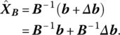
If this new basic solution is primal feasible ![]() , then, since
, then, since ![]() is independent of
is independent of ![]() , primal optimality or dual feasibility is also preserved. For Δb′ = (Δb1, …, Δbm), (8.6) becomes
, primal optimality or dual feasibility is also preserved. For Δb′ = (Δb1, …, Δbm), (8.6) becomes
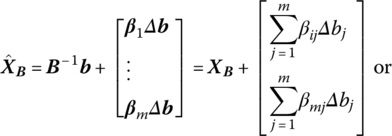
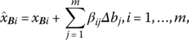
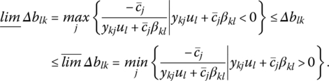
where βi = (βi1, …, βim), i = 1, …, m, denotes the ith row of B−1. Let us assume that bk changes. In order for this change to ensure the feasibility of the resulting basic solution, we require, by virtue of (8.7.1), that
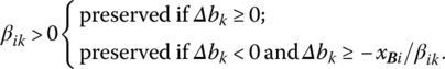
Under what conditions do changes in bk preserve the sense of this inequality? First, if βik = 0, then (8.7.2) holds for any Δbk. Second, for βik > 0, (8.7.2) is satisfied if Δbk ≥ 0, i.e. Δbk may increase without bound so that its upper limit is +∞. Thus, the feasibility of the new solution is affected only when Δbk < 0. Since (8.7.2) implies that −xBi/βik ≤ Δbk, i = 1, …, m, it follows that the lower limit to which Δbk can decrease without violating primal feasibility is −xBi/βik, βik > 0. Hence xBi remains in the set of basic variables as long as bk does not decrease by more than −xBi/βik. If βik > 0 for two or more basic variables xBi, then, to ensure that (8.7.2) is satisfied for all such i, the lower limit to which Δbk can decrease without violating the feasibility of the new primal solution is
Finally, if βik < 0, (8.7.2) holds if Δbk < 0, i.e. Δbk can decrease without bound so that its lower limit is −∞. Thus, the feasibility of the new basic solution is affected by changes in bk only when Δbk > 0. In this instance (8.7.2) may be rewritten as −xBi/βik ≥ Δbk, i = 1, …, m, so that the upper limit to Δbk is −xBi/βik, βik < 0. Hence xBi maintains its basic status provided that bk does not increase by more than −xBi/βik. And if βik < 0 for more than one basic variable xBi, then (8.7.2) holds for all relevant i if the upper limit to which Δbk can increase is specified as
If we choose to combine the lower and upper limits (8.8), (8.9), respectively, into a single expression, then (8.7.2) will be maintained if
Hence (8.10) provides the bounds within which Δbk may decrease or increase without affecting the feasibility of ![]() As an alternative to (8.10), we may express the limits contained therein in terms of the new level of bk, call it
As an alternative to (8.10), we may express the limits contained therein in terms of the new level of bk, call it ![]() by noting that, since
by noting that, since ![]()

What about the effect of a change in a component of the requirements vector on the optimal value of the objective function? By virtue of the preceding discussion, if (8.10) or (8.10.1) is satisfied, those variables that are currently basic remain so. However, a change in any of the requirements bi, i = 1. …, m, alters the optimal values of these variables, which in turn affect the optimal value of f. If bk alone changes, the magnitude of the change in f precipitated by a change in bk is simply Δf = ukΔbk since, as noted in Chapter 6, uk = Δf/Δbk represents a measure of the amount by which the optimal value of the primal objective function changes per unit change in the kth requirement bk.
Table 8.3 Limits within which b1, b2 can decrease or increase without violating primal optimality.
| Basic variables | Original requirements | Lower limit | Upper limit |
| xB1 = x3 | b1 = 100 | b1 − xB1/β11 = 26.67 | b1 − xB2/β21 = 320 |
| xB2 = x2 | b2 = 80 | b2 − xB2/β22 = 25 | b2 − xB1/β12 = 300 |
8.2.3 Changing a Component of the Coefficient Matrix
We now look to the effect on the optimal solution of a change in a component of the coefficient matrix ![]() associated with the structural constraint system
associated with the structural constraint system ![]() Since
Since ![]() was previously partitioned as
was previously partitioned as ![]() it may be the case that some component rij, i = 1, …, m; j = 1, …, n − m, of a nonbasic vector rj changes; or a component bki, i, k = 1, …, m, of a basic vector bi changes.
it may be the case that some component rij, i = 1, …, m; j = 1, …, n − m, of a nonbasic vector rj changes; or a component bki, i, k = 1, …, m, of a basic vector bi changes.
Let us begin by assuming that the lth component of the nonbasic vector ![]() changes to
changes to ![]() so that rk is replaced by
so that rk is replaced by ![]() Hence the matrix of nonbasic vectors may now be expressed as
Hence the matrix of nonbasic vectors may now be expressed as ![]() With
With ![]() independent of Δrlk at a basic feasible solution (since
independent of Δrlk at a basic feasible solution (since ![]() ), it follows that this nonbasic solution is primal feasible while, if
), it follows that this nonbasic solution is primal feasible while, if ![]() dual feasibility or primal optimality is also preserved. Since
dual feasibility or primal optimality is also preserved. Since

and ![]() it is evident that primal optimality is maintained if
it is evident that primal optimality is maintained if
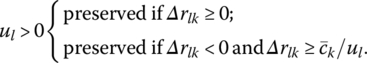
Under what circumstances will changes in rlk preserve the sense of this inequality? First, if ul = 0, then (8.12) holds regardless of the direction or magnitude of the change in rlk. Second, for ul > 0, (8.12) is satisfied if Δrlk ≥ 0, i.e. Δrlk may increase without bound so that its upper limit becomes +∞. Hence (8.12) is affected only when rlk decreases or Δrlk < 0. Since (8.12) implies that ![]() it is evident that the lower limit to which Δrlk can decrease without violating optimality is
it is evident that the lower limit to which Δrlk can decrease without violating optimality is ![]() Thus,
Thus, ![]() enters the basis (or
enters the basis (or ![]() enters the set of basic variables) only if the decrease in rlk is greater than
enters the set of basic variables) only if the decrease in rlk is greater than ![]() If we express this lower limit in terms of the new level of
If we express this lower limit in terms of the new level of ![]() then, for
then, for ![]()
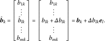
Next, let us assume that the lth component of the basis vector ![]() changes to
changes to ![]() so that bk is replaced in the basis matrix B = [b1, …, bk, …, bm] by
so that bk is replaced in the basis matrix B = [b1, …, bk, …, bm] by
Hence our initial problem becomes one of obtaining the inverse of the new basis matrix ![]() Then once
Then once ![]() is known, it can be shown that
is known, it can be shown that
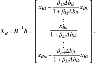
For ![]() primal feasible, we require that
primal feasible, we require that
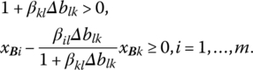
If 1 + βklΔblk > 0, then upon solving the second inequality for Δblk,

Since these inequalities must hold for all i ≠ k when 1 + βklΔblk > 0, the lower and upper limits to which Δblk can decrease or increase without violating primal feasibility may be expressed, from (8.14 a, b), respectively, as
If we re‐express these limits in terms of the new level of ![]() then, for
then, for ![]() (8.15) becomes
(8.15) becomes
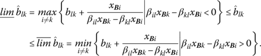
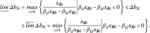
What is the effect of a change in blk upon the primal optimality (dual feasibility) requirement ![]() ? Here, too, it can be shown that the lower and upper limits to which Δblk can decrease or increase without violating primal optimality may be written as
? Here, too, it can be shown that the lower and upper limits to which Δblk can decrease or increase without violating primal optimality may be written as
Alternatively, we may write these limits in terms of the new level of ![]() since, if
since, if ![]() (8.16) becomes
(8.16) becomes

We next determine the effect of a change in the element blk upon the optimal value of the objective function. Again dispensing with the derivation we have the result that the new value of f is
Table 8.4 Limits to which r11, r21 can decrease or increase without violating primal optimality. Table 8.5 Limits to which b11, b21, b12 and b22 can decrease or increase without violating primal feasibility. Table 8.6 Limits to which b11, b21, b12, and b22 can decrease or increase without violating primal optimality. Table 8.7 Limits within which b11, b21, b12, and b22 can decrease or increase, without violating either primal feasibility or optimality.
Component of r1
Lower limit
Upper limit
r11 = 2
![]()
+∞
r21 = 1
![]()
+∞
Component of bi, i = 1, 2
Lower limit
Upper limit
b11 = 4
![]()
+∞
b21 = 1
−∞
![]()
b12 = 1
−∞
![]()
b22 = 3
![]()
+∞
Component of bi, i = 1, 2
Lower limit
Upper limit
b11 = 4
![]()
![]()
b21 = 1
−∞
![]()
b12 = 1
−∞
![]()
b22 = 3
![]()
+∞
Component of bi, i = 1, 2
Lower limit
Upper limit
b11 = 4
1.34
5.33
b21 = 1
−∞
2
b12 = 1
−∞
2
b22 = 3
0.80
+∞
8.3 Summary of Sensitivity Effects
- Changing an Objective Function Coefficient.
- Primal feasibility. Always preserved.
- Primal optimality.
- Changing the coefficient cRj of a nonbasic variable xRj:
- preserved if ΔcRj < 0.
- preserved if
- Changing the coefficient cBk of a basic variable xBk:
- preserved if ykj = 0.
-

- preserved if more than one

-
- preserved if more than one

- Changing the coefficient cRj of a nonbasic variable xRj:
- Changing a Component of the Requirement Vector.
- Primal optimality. Always preserved.
- Primal feasibility, i.e. conditions under which all xBi ≥ 0. Changing the requirement bk:
- preserved if βik = 0.
-
- preserved if more than one

-

- preserved if more than one

- Changing a Component of an Activity Vector.
- Changing a Component rlk of a Nonbasic Activity Vector rk.
- Primal feasibility. Always preserved.
- Primal optimality:
- Preserved if ul = 0.
-
- Changing a Component blk of a Basic Activity Vector bk.
- Primal feasibility, i.e. conditions under which all xBi ≥ 0.

- Primal optimality, i.e. conditions under which all


- Primal feasibility, i.e. conditions under which all xBi ≥ 0.
- Changing a Component rlk of a Nonbasic Activity Vector rk.