10
Parametric Programming
10.1 Introduction
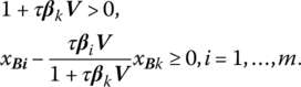
In Chapter 8 we considered an assortment of post‐optimality problems involving discrete changes in only selected components of the matrices ![]() Therein emphasis was placed on the extent to which a given problem may be modified without breaching its feasibility or optimality. We now wish to extend this sensitivity analysis a bit further to what is called parametric analysis. That is, instead of just determining the amount by which a few individual components of the aforementioned matrices may be altered in some particular way before the feasibility or optimality of the current solution is violated, let us generate a sequence of basic solutions that, in turn, become optimal, one after the other, as all of the components of
Therein emphasis was placed on the extent to which a given problem may be modified without breaching its feasibility or optimality. We now wish to extend this sensitivity analysis a bit further to what is called parametric analysis. That is, instead of just determining the amount by which a few individual components of the aforementioned matrices may be altered in some particular way before the feasibility or optimality of the current solution is violated, let us generate a sequence of basic solutions that, in turn, become optimal, one after the other, as all of the components of ![]() b, or a column of
b, or a column of ![]() vary continuously in some prescribed direction. In this regard, the following parametric analysis will involve a marriage between sensitivity analysis and simplex pivoting.
vary continuously in some prescribed direction. In this regard, the following parametric analysis will involve a marriage between sensitivity analysis and simplex pivoting.
10.2 Parametric Analysis
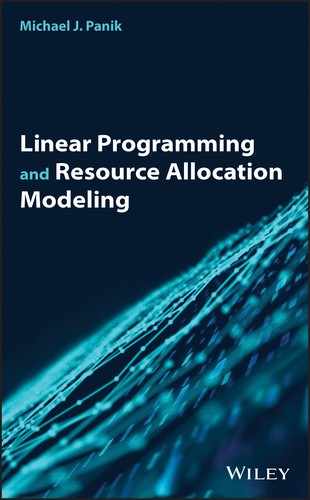
If we seek to
then an optimal basic feasible solution emerges if XB = B−1b ≥ O and ![]() (or, in terms of the optimal simplex matrix
(or, in terms of the optimal simplex matrix ![]() ) with
) with ![]() Given this result as our starting point, let us examine the process of parameterizing the objective function.
Given this result as our starting point, let us examine the process of parameterizing the objective function.
10.2.1 Parametrizing the Objective Function
Given the above optimal basic feasible solution, let us replace ![]() by
by ![]() where θ is a nonnegative scalar parameter and S is a specified, albeit arbitrary, (n × 1) vector that determines a given direction of change in the coefficients cj, j = 1, …, n. In this regard, the c*j, j = 1, …, n, are specified as linear functions of the parameter θ. Currently,
where θ is a nonnegative scalar parameter and S is a specified, albeit arbitrary, (n × 1) vector that determines a given direction of change in the coefficients cj, j = 1, …, n. In this regard, the c*j, j = 1, …, n, are specified as linear functions of the parameter θ. Currently, ![]() or
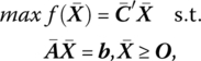
or ![]() If C* is partitioned as
If C* is partitioned as
where SB (SR) contains the components of S corresponding to the components of ![]() within CB(CR), then, when C* replaces
within CB(CR), then, when C* replaces ![]() . The revised optimality condition becomes
. The revised optimality condition becomes

or, in terms of the individual components of (10.1),
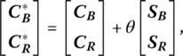
(Note that the parametrization of f affects only primal optimality and not primal feasibility since XB is independent of ![]() .) Let us now determine the largest value of θ (known as its critical value, θc) for which (10.1.1) holds. Upon examining this expression, it is evident that the critical value of θ is that for which any increase in θ beyond θc makes at least one of the
.) Let us now determine the largest value of θ (known as its critical value, θc) for which (10.1.1) holds. Upon examining this expression, it is evident that the critical value of θ is that for which any increase in θ beyond θc makes at least one of the ![]() values negative, thus violating optimality.
values negative, thus violating optimality.
How large of an increase in θ preserves optimality? First, if ![]() or
or ![]() the θ can be increased without bound while still maintaining the revised optimality criterion since, in this instance, (10.1.1) reveals that
the θ can be increased without bound while still maintaining the revised optimality criterion since, in this instance, (10.1.1) reveals that ![]() Next, if
Next, if ![]() for some particular value of j, then
for some particular value of j, then ![]() for
for
Hence, the revised optimality criterion is violated when θ > θc for some nonbasic variable xRj. Moreover, if ![]() for two or more nonbasic variables, then
for two or more nonbasic variables, then
So if θ increases and the minimum in (10.2) is attained for j = k, it follows that ![]() or
or ![]() With
With ![]() the case of multiple optimal basic feasible solutions obtains, i.e. the current basic feasible solution (call it
the case of multiple optimal basic feasible solutions obtains, i.e. the current basic feasible solution (call it ![]() ) remains optimal and the alternative optimal basic feasible solution (denoted
) remains optimal and the alternative optimal basic feasible solution (denoted ![]() ) emerges when rk is pivoted into the basis (or xRk enters the set of basic variables). And as θ increases slightly beyond θc,
) emerges when rk is pivoted into the basis (or xRk enters the set of basic variables). And as θ increases slightly beyond θc, ![]() so that
so that ![]() becomes the unique optimal basic feasible solution.
becomes the unique optimal basic feasible solution.
What about the choice of the direction vector S? As indicated above, S represents the direction in which the objective function coefficients are varied. So while the components of S are quite arbitrary (e.g. some of the cj values may be increased while others are decreased), it is often the case that only a single objective function coefficient cj is to be changed, i.e. S = ej (or −ej). Addressing ourselves to this latter case, if ![]() and xk is the nonbasic variable xRk, then (10.1.1) reduces to
and xk is the nonbasic variable xRk, then (10.1.1) reduces to ![]() for j ≠ k; while for j = k,
for j ≠ k; while for j = k, ![]() If θ increases so that
If θ increases so that ![]() or
or ![]() then the preceding discussion dictates that the column within the simplex matrix associated with xk is to enter the basis, with no corresponding adjustment in the current value of f warranted. Next, if xk is the basic variable xBk, (10.1.1) becomes
then the preceding discussion dictates that the column within the simplex matrix associated with xk is to enter the basis, with no corresponding adjustment in the current value of f warranted. Next, if xk is the basic variable xBk, (10.1.1) becomes ![]() In this instance (10.2) may be rewritten as
In this instance (10.2) may be rewritten as
If the minimum in (10.2.1) is attained for j = r, then ![]() Then rr may be pivoted into the basis so that, again, the case of multiple optimal basic feasible solutions holds. Furthermore, when xRr is pivoted into the set of basic variables, the current value of f must be adjusted by an amount Δf = ΔcBkxk = θcxBk as determined in Chapter 8.
Then rr may be pivoted into the basis so that, again, the case of multiple optimal basic feasible solutions holds. Furthermore, when xRr is pivoted into the set of basic variables, the current value of f must be adjusted by an amount Δf = ΔcBkxk = θcxBk as determined in Chapter 8.
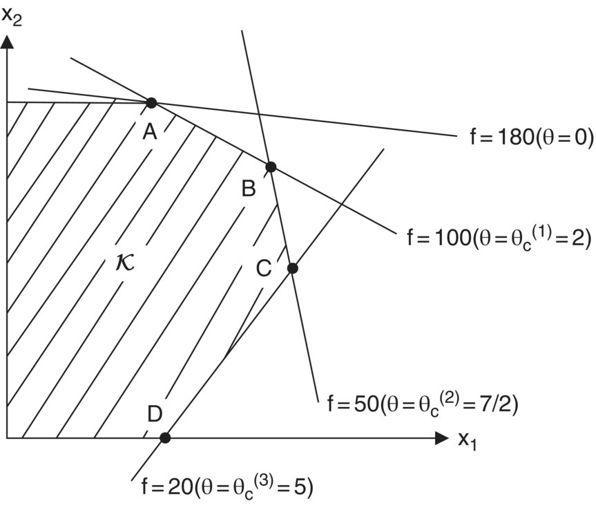
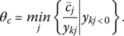
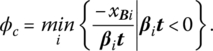
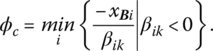
Figure 10.1 Generating the sequence A, B, C, and D of optimal extreme points parametrically.
Figure 10.2 Parametric path of x1, x2, and max f.
10.2.2 Parametrizing the Requirements Vector
Given that our starting point is again an optimal basic feasible solution to a linear programming problem, let us replace b by b* = b + φt, where φ is a nonnegative scalar parameter and t is a given (arbitrary) (m × 1) vector that specifies the direction of change in the requirements bi, i = 1, …, m. Hence, the ![]() vary linearly with the parameter φ. Currently, primal feasibility holds for XB = B−1b ≥ O or xBi ≥ 0, i = 1, …, m. With b* replacing b, the revised primal feasibility requirement becomes
vary linearly with the parameter φ. Currently, primal feasibility holds for XB = B−1b ≥ O or xBi ≥ 0, i = 1, …, m. With b* replacing b, the revised primal feasibility requirement becomes
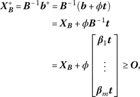
where βi devotes the ith row of B−1. In terms of the individual components of (10.3),
(Since the optimality criterion is independent of b, the parametrization of the latter affects only primal feasibility and not primal optimality.) What is the largest value of φ for which (10.3.1) holds? Clearly the implied critical value of φ, φc, is that for which any increase in φ beyond φc violates feasibility, i.e. makes at least one of the ![]() values negative.
values negative.
To determine φc, let us first assume that βit ≥ 0, i = 1, …, m. Then φ can be increased without bound while still maintaining the revised feasibility criterion since, in this instance, ![]() Next, if βit < 0 for some i,
Next, if βit < 0 for some i, ![]() for
for
Hence, the revised feasibility criterion is violated when φ > φc for some basic variable xBi. Moreover, if βit < 0 for two or more basic variables, then
Now, if φ increases and the minimum in (10.4) is attained for i = k, it follows that ![]() And as φ increases beyond
And as φ increases beyond ![]() so that bk must be removed from the basis to preserve primal feasibility, with its replacement vector determined by the dual simplex entry criterion.
so that bk must be removed from the basis to preserve primal feasibility, with its replacement vector determined by the dual simplex entry criterion.
Although the specification of the direction vector t is arbitrary, it is frequently the case that only a single requirement bi is to be changed, so that t = ei(or − ei). With respect to this particular selection of t, if b* = b + φek, then (10.3.1) simplifies to ![]() For this choice of t then, (10.4) may be rewritten as
For this choice of t then, (10.4) may be rewritten as
If the minimum in (10.4.1) is attained for ![]() If φ then increases above this critical value,
If φ then increases above this critical value, ![]() turns negative so that bl is pivoted out of the basis to maintain primal feasibility. Moreover, as bk changes, f must be modified by an amount Δf = ukΔbk = ukφc.
turns negative so that bl is pivoted out of the basis to maintain primal feasibility. Moreover, as bk changes, f must be modified by an amount Δf = ukΔbk = ukφc.

Figure 10.3 Generating the sequence B, E, and F of optimal extreme points parametrically.


Figure 10.4 Parametric path of x1, x2, b3, and max f.
One final point is in order. In the preceding two example problems, we parametrized b directly. However, if we consider the associated dual problems, then parametrizing b can be handled in the same fashion as parametrizing the objective function.
10.2.3 Parametrizing an Activity Vector
Given that we have obtained an optimal basic feasible solution to the problem
let us undertake the parametrization of a column of the activity matrix ![]() With
With ![]() previously partitioned as
previously partitioned as ![]() it may be the case that: some nonbasic vector rj is replaced by
it may be the case that: some nonbasic vector rj is replaced by ![]() or a basic vector bi is replaced by
or a basic vector bi is replaced by ![]() where τ represents a nonnegative scalar parameter and V is an arbitrary (m × 1) vector that determines the direction of change in the components of either rj or bi. In each individual case, the said components are expressed as linear functions of τ.
where τ represents a nonnegative scalar parameter and V is an arbitrary (m × 1) vector that determines the direction of change in the components of either rj or bi. In each individual case, the said components are expressed as linear functions of τ.
Let us initially assume that rk is replaced by ![]() in R = [r1, …, rk, …, rn − m] so that the new matrix of nonbasic vectors appears as
in R = [r1, …, rk, …, rn − m] so that the new matrix of nonbasic vectors appears as ![]() Since the elements within the basis matrix B are independent of the parametrization of rk, primal feasibility is unaffected (we still have XB = B−1b ≥ O) but primal optimality may be compromised. In this regard, for
Since the elements within the basis matrix B are independent of the parametrization of rk, primal feasibility is unaffected (we still have XB = B−1b ≥ O) but primal optimality may be compromised. In this regard, for ![]()
![]() Upon parametrizing rk, the revised optimality criterion becomes
Upon parametrizing rk, the revised optimality criterion becomes
where
and ![]() is a (1 × m) vector of nonnegative dual variables. Since
is a (1 × m) vector of nonnegative dual variables. Since ![]() primal optimality will be preserved if (10.5) holds. Now, as τ increases, primal optimality must be maintained. Given this restriction, what is the largest value of τ (its critical value, τc) for which (10.5) holds?
primal optimality will be preserved if (10.5) holds. Now, as τ increases, primal optimality must be maintained. Given this restriction, what is the largest value of τ (its critical value, τc) for which (10.5) holds?
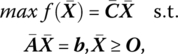
To find τc, we shall first assume that U′V ≥ 0. Then τ can be increased indefinitely while still maintaining the revised optimality criterion. Next, if U′V < 0, then ![]() for
for
In this regard, as τ increases to τc, it follows that ![]() so that the case of multiple optimal solutions emerges. That is, the current basic feasible solution (call it
so that the case of multiple optimal solutions emerges. That is, the current basic feasible solution (call it ![]() ) remains optimal and an alternative optimal basic feasible solution (
) remains optimal and an alternative optimal basic feasible solution (![]() ) obtains when rk is pivoted into the basis, with the primal simplex criterion determining the vector to be removed from the current basis. And as τ increases a bit beyond τc, it follows that
) obtains when rk is pivoted into the basis, with the primal simplex criterion determining the vector to be removed from the current basis. And as τ increases a bit beyond τc, it follows that ![]() so that
so that ![]() becomes the unique optimal basic feasible solution.
becomes the unique optimal basic feasible solution.
As indicated above, the choice of the direction vector V is completely arbitrary. However, if only a single component rik of the activity vector rk is to change, then V = ei(or − ei). In this regard, if ![]() then (10.5) becomes
then (10.5) becomes ![]() So for this choice of V, with ul ≥ 0, τ may be increased without bound while still preserving primal optimality. Next if
So for this choice of V, with ul ≥ 0, τ may be increased without bound while still preserving primal optimality. Next if ![]() (10.5) simplifies to
(10.5) simplifies to ![]() In this instance, (10.6) may be rewritten as
In this instance, (10.6) may be rewritten as
If τ then increases above this critical value, ![]() turns negative so that rk is pivoted into the basis to maintain primal optimality.
turns negative so that rk is pivoted into the basis to maintain primal optimality.
When τ is increased slightly above ![]() it may be the case that: τ may be increased without bound while still preserving primal optimality; or there exists a second critical value of τ beyond which the new basis ceases to yield an optimal feasible solution. Relative to this latter instance, since rk has entered the optimal basis, we now have to determine a procedure for parametrizing a basis vector. Before doing so, however, let us examine Example 10.4.
it may be the case that: τ may be increased without bound while still preserving primal optimality; or there exists a second critical value of τ beyond which the new basis ceases to yield an optimal feasible solution. Relative to this latter instance, since rk has entered the optimal basis, we now have to determine a procedure for parametrizing a basis vector. Before doing so, however, let us examine Example 10.4.
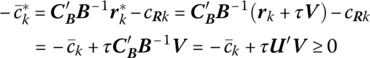
Next, to parametrize a vector within the optimal basis, let us replace the kth column bk of the basis matrix ![]() so as to obtain
so as to obtain ![]() Since
Since ![]() it follows that
it follows that

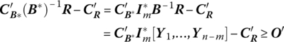
From (10.A.1) of Appendix 10.A,
And from (10.A.2), ![]() and thus
and thus

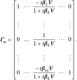
Since ![]() must be primal feasible, we require that
must be primal feasible, we require that
If 1 + τβkV > 0, then, upon solving the second inequality for τ and remembering that τ must be strictly positive,
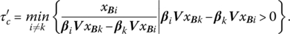
Since (10.7) must hold for all i ≠ k when 1 + τβkV > 0, it follows that the upper limit or critical value to which τ can increase without violating primal feasibility is
To determine the effect of parametrizing the basis vector upon primal optimality, let us express the revised optimality criterion as
or, in terms of its components

If we now add and subtract the term
on the left‐hand side of (10.9), the latter simplifies to
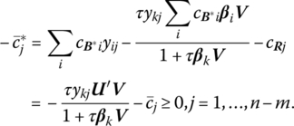
If 1 + τβkV > 0, and again remembering that τ must be strictly positive, we may solve (10.9.1) for τ as
Since (10.10) is required to hold for all j = 1, …, n − m when 1 + τβkV > 0, we may write the critical value to which τ can increase while still preserving primal optimality as

As we have just seen, the parametrization of a basis vector may affect both the feasibility and optimality of the current solution. This being the case, the critical value of τ that preserves both primal feasibility and optimality simultaneously is simply
Finally, the effect on the optimal value of f parametrizing bk can be shown to be
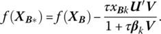
As far as the specification of the arbitrary direction vector V is concerned, it is sometimes the case that only a single component of bi is to change, i.e. V = ei (or − ei) so that ![]()
Now that we have seen how the various component parts of the primal program can be parametrized, we turn to Chapter 11 where the techniques developed in this chapter are applied in deriving output supply functions; input demand functions; marginal revenue productivity functions; marginal, total, and variable cost functions; and marginal and average productivity functions.
10.A Updating the Basis Inverse
We know that to obtain a new basic feasible solution to a linear programming problem via the simplex method, we need change only a single vector in the basis matrix at each iteration. We are thus faced with the problem of finding the inverse of a matrix ![]() that has only one column different from that of a matrix B whose inverse is known. So given B = [b1, …, bm] with B−1 known, we wish to replace the rth column br of B by rj so as obtain the inverse of
that has only one column different from that of a matrix B whose inverse is known. So given B = [b1, …, bm] with B−1 known, we wish to replace the rth column br of B by rj so as obtain the inverse of ![]() Since the columns of B form a basis for Rm, rj = BYj. If the columns of
Since the columns of B form a basis for Rm, rj = BYj. If the columns of ![]() are also to yield a basis for Rm, then it must be true that yrj ≠ 0. So if
are also to yield a basis for Rm, then it must be true that yrj ≠ 0. So if

with yrj ≠ 0, then

 Hence br has been removed from the basis with rj entered in its stead. If we next replace the rth column of the mth order identity matrix
 ![]() we obtain
we obtain
where, as previously defined, ej is the jth unit column vector. Now it is easily demonstrated that ![]() so that
so that