
Chapter 9
Calibration Techniques
One of the key challenges in steganalysis is that most features vary a lot within each class, and sometimes more than between classes. What if we could calibrate the features by estimating what the feature would have been for the cover image?
Several such calibration techniques have been proposed in the literature. We will discuss two of the most well-known ones, namely the JPEG calibration of Fridrich et al. (2002) and calibration by downsampling as introduced by Ker (2005b). Both of these techniques aim to estimate the features of the cover image. In Section 9.4, we will discuss a generalisation of calibration, looking beyond cover estimates.
9.1 Calibrated Features
We will start by considering calibration techniques aiming to estimate the features of the cover image, and introduce key terminology and notation.
We view a feature vector as a function ![]() , where
, where ![]() is the image space (e.g.
is the image space (e.g. ![]() for 8-bit grey-scale images). A reference transform is any function
for 8-bit grey-scale images). A reference transform is any function ![]() . Given an image
. Given an image ![]() , the transformed image
, the transformed image ![]() is called the reference image.
is called the reference image.
If, for any cover image ![]() and any corresponding steganogram
and any corresponding steganogram ![]() , we have
, we have
9.1 ![]()
we say that ![]() is a cover estimate with respect to
is a cover estimate with respect to ![]() . This clearly leads to a discriminant if additionally
. This clearly leads to a discriminant if additionally ![]() . We could then simply compare
. We could then simply compare ![]() and
and ![]() of an intercepted image
of an intercepted image ![]() . If
. If ![]() we can assume that the image is clean; otherwise it must be a steganogram.
we can assume that the image is clean; otherwise it must be a steganogram.
The next question is how we can best quantify the relationship between ![]() and
and ![]() to get some sort of calibrated features. Often it is useful to take a scalar feature
to get some sort of calibrated features. Often it is useful to take a scalar feature ![]() and use it to construct a scalar calibrated feature
and use it to construct a scalar calibrated feature ![]() as a function of
as a function of ![]() and
and ![]() . In this case, two obvious choices are the difference or the ratio:
. In this case, two obvious choices are the difference or the ratio:
where ![]() is a scalar. Clearly, we would expect
is a scalar. Clearly, we would expect ![]() and
and ![]() for a natural image
for a natural image ![]() , and some other value for a steganogram. Depending on the feature
, and some other value for a steganogram. Depending on the feature ![]() , we may or may not know if the calibrated feature of a steganogram is likely to be smaller or greater than that of a natural image.
, we may or may not know if the calibrated feature of a steganogram is likely to be smaller or greater than that of a natural image.
The definition of ![]() clearly extends to a vector function
clearly extends to a vector function ![]() ; whereas
; whereas ![]() would have to take the element-wise ratio for a vector function, i.e.
would have to take the element-wise ratio for a vector function, i.e.
We will refer to ![]() as a difference calibrated feature and to
as a difference calibrated feature and to ![]() as a ratio calibrated feature.
as a ratio calibrated feature.
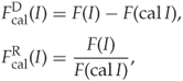
Figure 9.1 illustrates the relationship we are striving for in a 2-D feature space. The original feature vectors, ![]() and
and ![]() , indicated by dashed arrows are relatively similar, both in angle and in magnitude. Difference calibration gives us feature vectors
, indicated by dashed arrows are relatively similar, both in angle and in magnitude. Difference calibration gives us feature vectors ![]() and
and ![]() , indicated by solid arrows, that are
, indicated by solid arrows, that are ![]() –
–![]() apart. There is a lot of slack in approximating
apart. There is a lot of slack in approximating ![]() for the purpose of illustration.
for the purpose of illustration.
Figure 9.1 Suspicious image and (difference) calibrated image in feature space
Calibration can in principle be applied to any feature ![]() . However, a reference transform may be a cover estimate for one feature vector
. However, a reference transform may be a cover estimate for one feature vector ![]() , and not for another feature vector
, and not for another feature vector ![]() . Hence, one calibration technique cannot be blindly extended to new features, and has to be evaluated for each feature vector considered.
. Hence, one calibration technique cannot be blindly extended to new features, and has to be evaluated for each feature vector considered.
The ratio and difference have similar properties, but the different scales may very well make a serious difference in the classifier. We are not aware of any systematic comparison of the two in the literature, whether in general or in particular special cases. Fridrich (2005) used the difference of feature vectors, and Ker (2005b) used the ratio of scalar discriminants.
The calibrated features ![]() and
and ![]() are clearly good discriminants if the approximation in (9.1) is good and the underlying feature
are clearly good discriminants if the approximation in (9.1) is good and the underlying feature ![]() has any discriminating power whatsoever. Therefore, it was quite surprising when Kodovský and Fridrich (2009) re-evaluated the features of Pevný and Fridrich (2007) and showed that calibration actually leads to inferior classification. The most plausible explanation is that the reference transform is not a good cover estimate for all images and for all the features considered.
has any discriminating power whatsoever. Therefore, it was quite surprising when Kodovský and Fridrich (2009) re-evaluated the features of Pevný and Fridrich (2007) and showed that calibration actually leads to inferior classification. The most plausible explanation is that the reference transform is not a good cover estimate for all images and for all the features considered.
The re-evaluation by Kodovský and Fridrich (2009) led to the third approach to feature calibration, namely the Cartesian calibrated feature. Instead of taking a scalar function of the original and calibrated features, we simply take both, as the Cartesian product ![]() for each scalar feature
for each scalar feature ![]() . The beauty of this approach is that no information is discarded, and the learning classifier can use all the information contained in
. The beauty of this approach is that no information is discarded, and the learning classifier can use all the information contained in ![]() and
and ![]() for training. Calibration then becomes an implicit part of learning. We will return to this in more detail in Section 9.2.2.
for training. Calibration then becomes an implicit part of learning. We will return to this in more detail in Section 9.2.2.
9.2 JPEG Calibration
The earliest and most well-known form of calibration is JPEG calibration. The idea is to shift the ![]() grid by half a block. The embedding distortion, following the original
grid by half a block. The embedding distortion, following the original ![]() grid, is assumed to affect features calculated along the original grid only. This leads to the following algorithm.
grid, is assumed to affect features calculated along the original grid only. This leads to the following algorithm.
JPEG calibration was introduced for the blockiness attack, using 1-norm blockiness as the only feature. The technique was designed to be a cover estimate, and the original experiments confirmed that it is indeed a cover estimate with respect to blockiness. The reason why it works is that blockiness is designed to detect the discontinuities on the block boundaries caused by independent noise in each block. By shifting the grid, we get a compression domain which is independent of the embedding domain, and the discontinuities at the boundaries are expected to be weaker. This logic does not necessarily apply for other features.
9.2.1 The FRI-23 Feature Set
The idea of using JPEG calibration with learning classifiers was introduced by Fridrich (2005), creating a 23-dimensional feature vector which we will call FRI-23. Most of the 23 features are created by taking the 1-norm ![]() of an underlying, multi-dimensional, difference calibrated feature vector, as follows.
of an underlying, multi-dimensional, difference calibrated feature vector, as follows.
![]()
Note that this definition applies to a scalar feature ![]() as well, where the
as well, where the ![]() -norm reduces to the absolute value
-norm reduces to the absolute value ![]() . The features underlying FRI-23 are the same as for NCPEV-219, as we discussed in Chapter 8. Fridrich used 17 multi-dimensional feature vectors and three scalar features, giving rise to 20 features using Definition 9.2.2. She used a further three features not based on this definition. The 23 features are summarised in Table 9.1. The variation and blockiness features are simply the difference calibrated features from
. The features underlying FRI-23 are the same as for NCPEV-219, as we discussed in Chapter 8. Fridrich used 17 multi-dimensional feature vectors and three scalar features, giving rise to 20 features using Definition 9.2.2. She used a further three features not based on this definition. The 23 features are summarised in Table 9.1. The variation and blockiness features are simply the difference calibrated features from ![]() ,
, ![]() and
and ![]() from NCPEV-219.
from NCPEV-219.
Table 9.1 Overview of the calibrated features used by Fridrich (2005) and Pevný and Fridrich (2007)
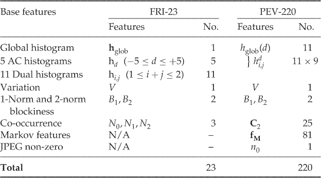
For the histogram features, Definition 9.2.2 allows us to include the complete histogram. Taking just the norm keeps the total number of features down. The feature vectors used are:
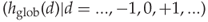 (global histogram);
 (dual histogram) for
  ; and
; and (per-frequency AC histograms) for
  .
.
Each of these feature vectors gives one calibrated feature. Note that even though the same underlying features occur both in the local and the dual histogram, the resulting Fridrich calibrated features are distinct.
The last couple of features are extracted from the co-occurrence matrix. These are special in that we use the signed difference, instead of the unsigned difference of the 1-norm in Definition 9.2.2.
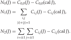
According to Fridrich, the co-occurrence matrix tends to be symmetric around ![]() , giving a strong positive correlation between
, giving a strong positive correlation between ![]() for
for ![]() and for
and for ![]() . Thus, the elements which are added for
. Thus, the elements which are added for ![]() and for
and for ![]() above will tend to enforce each other and not cancel each other out, making this a good way to reduce dimensionality.
above will tend to enforce each other and not cancel each other out, making this a good way to reduce dimensionality.
9.2.2 The Pevný Features and Cartesian Calibration
An important pioneer in promoting calibration techniques, FRI-23 seems to have too few features to be effective. Pevný and Fridrich (2007) used the difference-calibrated feature vector ![]() directly, instead of the Fridrich-calibrated features, where
directly, instead of the Fridrich-calibrated features, where ![]() is NCPEV-219.
is NCPEV-219.
The difference-calibrated features intuitively sound like a very good idea. However, in practice, they are not always as effective as they were supposed to be. Kodovský and Fridrich (2009) compared PEV-219 and NCPEV-219. Only for JP Hide and Seek did PEV-219 outperform NCPEV-219. For YASS, the calibrated features performed significantly worse. For the other four algorithms tested (nsF5, JSteg, Steghide and MME3), there was no significant difference.
The failure of difference-calibrated features led Kodovský and Fridrich to propose a Cartesian-calibrated feature vector, CCPEV-438, as the Cartesian product of NCPEV-219 calculated from the image ![]() and NCPEV-219 calculated from
and NCPEV-219 calculated from ![]() .
.
Table 9.2 shows some experimental results with different forms of calibration. The first test is based on Pevný's features, and it is not a very strong case for calibration of any kind. We compare the uncalibrated features (NCPEV-219), the difference-calibrated features (PEV-219), and the Cartesian features (PEV-438). We have also shown the features calculated only from ![]() as CPEV-219. We immediately see that the original uncalibrated features are approximately even with Cartesian calibration and better than difference calibration.
as CPEV-219. We immediately see that the original uncalibrated features are approximately even with Cartesian calibration and better than difference calibration.
Table 9.2 Comparison of accuracies of feature vectors for JPEG steganography
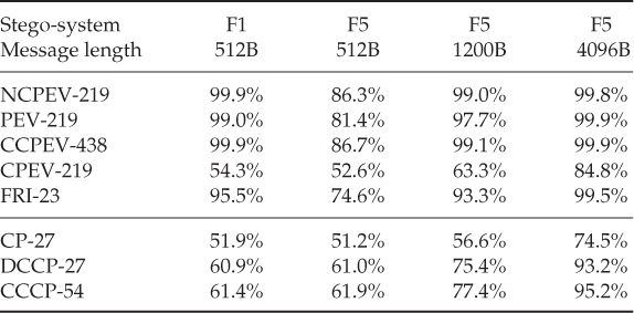
A better case for calibration is found by considering other features, like the conditional probability features CP-27. Calibrated versions improve the accuracy significantly in each of the cases tested. Another case for calibration was offered by Zhang and Zhang (2010), where the accuracy of the 243-D Markov feature vector was improved using Cartesian calibration.
When JPEG calibration does not improve the accuracy for NCPEV-219, the most plausible explanation is that it is not a good cover estimate. This is confirmed by the ability of CPEV-219 to discriminate between clean images and steganograms for long messages. This would have been impossible if ![]() . Thus we have confirmed what we hinted earlier, that although JPEG calibration was designed as a cover estimate with respect to blockiness, there is no reason to assume that it will be a cover estimate with respect to other features.
. Thus we have confirmed what we hinted earlier, that although JPEG calibration was designed as a cover estimate with respect to blockiness, there is no reason to assume that it will be a cover estimate with respect to other features.
JPEG calibration can also be used as a cover estimate with respect to the histogram (Fridrich et al., 2003b). It is not always very good, possibly because calibration itself introduce new artifacts, but it can be improved. A blurring filter applied to the decompressed image will even out the high-frequency noise caused by the original sub-blocking. Fridrich et al. (2003b) recommended applying the following blurring filter before recompression (between Steps 2 and 3 in Algorithm 9.2.1):
The resulting calibrated image had an AC histogram closely matching that of the original cover image, as desired.
9.3 Calibration by Downsampling
Downsampling is the action of reducing the resolution of a digital signal. In the simplest form a group of adjacent pixels is averaged to form one pixel in the downsampled image. Obviously, high-frequency information will be lost, while the low-frequency information will be preserved. Hence, one may assume that a downsampling of a steganogram ![]() will be almost equal to the downsampling of the corresponding cover image
will be almost equal to the downsampling of the corresponding cover image ![]() , as the high-frequency noise caused by embedding is lost. Potentially, this gives us a calibration technique, which has been explored by a number of authors.
, as the high-frequency noise caused by embedding is lost. Potentially, this gives us a calibration technique, which has been explored by a number of authors.
Ker (2005b) is the pioneer on calibration based on downsampling. The initial work was based on the HCF-COM feature of Harmsen (2003) (see Section 6.1.1). The problem with HCF-COM is that its variation, even within one class, is enormous, and even though it is statistically greater for natural images than for steganograms, this difference may not be significant. In this situation, calibration may give a baseline for comparison and to improve the discrimination.
Most of the work on downsampling has aimed to identify a single discriminating feature which in itself is able to discriminate between steganograms and clean images. This eliminates the need for a classification algorithm; only a threshold ![]() needs to be chosen. If
needs to be chosen. If ![]() is the discriminating feature, we predict one class label for
is the discriminating feature, we predict one class label for ![]() and the alternative class for
and the alternative class for ![]() . Therefore we will not discuss feature vectors in this section. However, there is no reason why one could not combine a number of the proposed statistics, or even intermediate quantities, into feature vectors for machine learning. We have not seen experiments on such feature vectors, and we leave it as an exercise for the reader.
. Therefore we will not discuss feature vectors in this section. However, there is no reason why one could not combine a number of the proposed statistics, or even intermediate quantities, into feature vectors for machine learning. We have not seen experiments on such feature vectors, and we leave it as an exercise for the reader.
9.3.1 Downsampling as Calibration
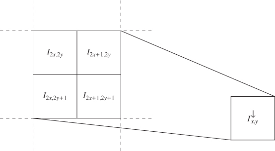
Ker (2005b) suggests downsampling by a factor of two in each dimension. Let ![]() denote the down sampled version of an image
denote the down sampled version of an image ![]() . Each pixel of
. Each pixel of ![]() is simply the average of four (
is simply the average of four (![]() ) pixels of
) pixels of ![]() , as shown in Figure 9.2. Mathematically we write
, as shown in Figure 9.2. Mathematically we write
Except for the rounding, this is equivalent to the low-pass component of a (2-D) Haar wavelet decomposition.
Figure 9.2 Downsampling á la Ker
Downsampling as calibration is based on the assumption that the embedding distortion ![]() is a random variable, identically and independently distributed for each pixel
is a random variable, identically and independently distributed for each pixel ![]() . Taking the average of four pixels, we reduce the variance of the distortion. To see this, compare the downsampled pixels of a clean image
. Taking the average of four pixels, we reduce the variance of the distortion. To see this, compare the downsampled pixels of a clean image ![]() and a steganogram
and a steganogram ![]() :
:
9.2 
9.3 
If ![]() are identically and independently distributed, the variance of
are identically and independently distributed, the variance of ![]() is a quarter of the variance of
is a quarter of the variance of ![]() . If
. If ![]() has zero mean, this translates directly to the distortion power on
has zero mean, this translates directly to the distortion power on ![]() being a quarter of the distortion power on
being a quarter of the distortion power on ![]() .
.
Intuitively one would thus expect downsampling to work as a cover estimate with respect to most features ![]() . In particular, we would expect that
. In particular, we would expect that
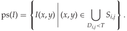
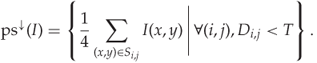
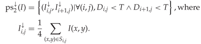
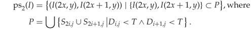
9.4 ![]()
9.5 ![]()
If this holds, a natural image can be recognised as having ![]() , whereas
, whereas ![]() for steganograms.
for steganograms.
We shall see later that this intuition is correct under certain conditions, whereas the rounding (floor function) in (9.3) causes problems in other cases. In order to explore this, we need concrete examples of features using calibration. We start with the HCF-COM.
9.3.2 Calibrated HCF-COM
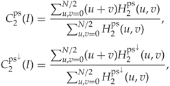
The initial application of downsampling for calibration (Ker, 2005b) aimed to adapt HCF-COM (Definition 4.3.5) to be effective for grey-scale images. We remember that Harmsen's original application of HCF-COM depended on the correlation between colour channels, and first-order HCF-COM features are ineffective on grey-scale images. Downsampling provides an alternative to second-order HCF-COM on grey-scale images. The ratio-calibrated HCF-COM feature used by Ker is defined as
![]()
where ![]() is the HCF-COM of image
is the HCF-COM of image ![]() . Ker's experiment showed that
. Ker's experiment showed that ![]() had slightly better accuracy than
had slightly better accuracy than ![]() against LSB
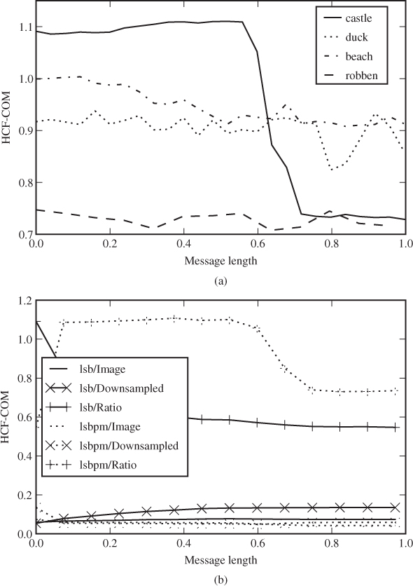
against LSB![]() at 50% of capacity, and significantly better at 100% of capacity. In Figure 9.3 we show how the HCF-COM features vary with the embedding rate for a number of images. Interestingly, we see that for some, but not all images,
at 50% of capacity, and significantly better at 100% of capacity. In Figure 9.3 we show how the HCF-COM features vary with the embedding rate for a number of images. Interestingly, we see that for some, but not all images, ![]() show a distinct fall around 50–60% embedding.
show a distinct fall around 50–60% embedding.
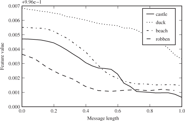
Figure 9.3 HCF-COM: (a) calibrated for various images; (b) calibrated versus non-calibrated
In Figure 9.3(b), we compare ![]() ,
, ![]() and
and ![]() for one of the images where
for one of the images where ![]() shows a clear fall. We observe that neither
shows a clear fall. We observe that neither ![]() nor
nor ![]() shows a similar dependency on the embedding rate, confirming the usefulness of calibration. However, we can also see that downsampling does not at all operate as a cover estimate, as
shows a similar dependency on the embedding rate, confirming the usefulness of calibration. However, we can also see that downsampling does not at all operate as a cover estimate, as ![]() can change more with the embedding rate than
can change more with the embedding rate than ![]() does.
does.
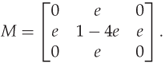
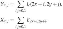
Ker (2005b) also considered the adjacency HCF-COM, as we discussed in Section 4.3. The calibrated adjacency HCF-COM is defined as the scalar feature ![]() given as
given as
Our experiments with uncompressed images in Figure 9.4 show a more consistent trend than we had with the regular HCF-COM.
Figure 9.4 Calibrated adjacency HCF-COM for various images
9.3.3 The Sum and Difference Images
Downsampling as calibration works well in some situations, where it is a reasonable cover estimate. In other situations, it is a poor cover estimate, even with respect to the features ![]() and
and ![]() . We will have a look at when this happens, and how to amend the calibration technique to be more robust.
. We will have a look at when this happens, and how to amend the calibration technique to be more robust.
We define
Clearly, we can rewrite (9.2) and (9.3) defining the downsampled images as ![]() and
and ![]() .
.
The critical question is the statistical distribution of ![]() . With a uniform distribution, both
. With a uniform distribution, both ![]() and
and ![]() will be close to 1 for natural images and significantly less for steganograms. Assuming that
will be close to 1 for natural images and significantly less for steganograms. Assuming that ![]() is uniformly distributed, Ker (2005a) was able to prove that
is uniformly distributed, Ker (2005a) was able to prove that
![]()
and it was verified empirically that
![]()
According to Ker, uniform distribution is typical for scanned images. However, images decompressed from JPEG would tend to have disproportionately many groups for which ![]() .
.
We can see that if ![]() , a positive embedding distortion
, a positive embedding distortion ![]() will disappear in the floor function in the definition of
will disappear in the floor function in the definition of ![]() , while negative distortion
, while negative distortion ![]() will carry through. This means that the embedding distortion
will carry through. This means that the embedding distortion ![]() is biased, with a negative expectation. It can also cause the distortion to be stronger in
is biased, with a negative expectation. It can also cause the distortion to be stronger in ![]() than in
than in ![]() , and not weaker as we expected. The exact effect has not been quantified in the literature, but the negative implications can be observed on some of the proposed features using calibration. They do not give good classifiers for previously compressed images.
, and not weaker as we expected. The exact effect has not been quantified in the literature, but the negative implications can be observed on some of the proposed features using calibration. They do not give good classifiers for previously compressed images.
The obvious solution to this problem is to avoid the rounding function in the definition ![]() :
:
In fact, the only reason to use this definition is to be able to treat ![]() as an image of the same colour depth as
as an image of the same colour depth as ![]() . However, there is no problem using the sum image
. However, there is no problem using the sum image
![]()
as the calibrated image. The only difference between ![]() and
and ![]() is that the latter has four times the colour depth, that is a range
is that the latter has four times the colour depth, that is a range ![]() if
if ![]() is an 8-bit image.
is an 8-bit image.
The increased colour depth makes ![]() computationally more expensive to use than
computationally more expensive to use than ![]() . If we want to calculate HAR3D-3, using a joint histogram across three colour channels and calculating a 3-D HCF using the 3-D DFT, the computational cost increases by a factor of 64 or more. A good compromise may be to calculate a sum image by adding pairs in one dimension only (Ker, 2005a), that is
. If we want to calculate HAR3D-3, using a joint histogram across three colour channels and calculating a 3-D HCF using the 3-D DFT, the computational cost increases by a factor of 64 or more. A good compromise may be to calculate a sum image by adding pairs in one dimension only (Ker, 2005a), that is
![]()
Thus the pixel range is doubled instead of quadrupled, saving some of the added computational cost of the DFT. For instance, when a 3-D DFT is used, the cost factor is 8 instead of 64.
The HCF of ![]() will have twice as many terms as that of
will have twice as many terms as that of ![]() , because of the increased pixel range. In order to get comparable statistics for
, because of the increased pixel range. In order to get comparable statistics for ![]() and for
and for ![]() , we can use only the lower half of frequencies for
, we can use only the lower half of frequencies for ![]() . This leads to Ker's (2005a) statistic
. This leads to Ker's (2005a) statistic
with ![]() for an 8-bit image
for an 8-bit image ![]() . It is the high-frequency components of the HCF of
. It is the high-frequency components of the HCF of ![]() that are discarded, meaning that we get rid of some high-frequency noise. There is no apparent reason why
that are discarded, meaning that we get rid of some high-frequency noise. There is no apparent reason why ![]() would not be applicable to grey-scale images, but we have only seen it used with colour images as discussed below in Section 9.3.4.
would not be applicable to grey-scale images, but we have only seen it used with colour images as discussed below in Section 9.3.4.
The discussion of 2-D histograms and difference matrices in Chapter 4 indicate that the greatest effect of embedding can be seen in the differences between neighbour pixels, rather than individual pixels or even pixel pairs. Pixel differences are captured by the high-pass Haar transform. We have already seen the sum image ![]() , which is a a low-pass Haar transform across one dimension only. The difference image can be defined as
, which is a a low-pass Haar transform across one dimension only. The difference image can be defined as
![]()
and it is a high-pass Haar transform across one dimension. Li et al. (2008a) suggested using both the difference and sum images, using the HCF-COM ![]() and
and ![]() as features. Experimentally, Li et al. show that
as features. Experimentally, Li et al. show that ![]() is a better detector than both
is a better detector than both ![]() and
and ![]() .
.
The difference matrix ![]() differs from the difference matrix of Chapter 4 in two ways. Firstly, the range is adjusted to be
differs from the difference matrix of Chapter 4 in two ways. Firstly, the range is adjusted to be ![]() instead of
instead of ![]() . Secondly, it is downsampled by discarding every other difference; we do not consider
. Secondly, it is downsampled by discarding every other difference; we do not consider ![]() . The idea is also very similar to wavelet analysis, except that we make sure to use an integer transform and use it only along one dimension.
. The idea is also very similar to wavelet analysis, except that we make sure to use an integer transform and use it only along one dimension.
Since the sum and difference images ![]() and
and ![]() correspond respectively to the low-pass and high-pass Haar wavelets applied in one dimension only, the discussion above, combined with the principles of Cartesian calibration, may well be used to justify features calculated from the wavelet domain.
correspond respectively to the low-pass and high-pass Haar wavelets applied in one dimension only, the discussion above, combined with the principles of Cartesian calibration, may well be used to justify features calculated from the wavelet domain.
9.3.4 Features for Colour Images
In the grey-scale case we saw good results with a two-dimensional adjacency HCF-COM. If we want to use this in the colour case, we can hardly simultaneously consider the three colour channels jointly, because of the complexity of a 6-D Fourier transform. One alternative would be to deal with each colour channel separately, to get three features.
Most of the literature on HCF-COM has aimed to find a single discriminating feature, and to achieve this Ker (2005a) suggested adding all the three colour components together and then taking the adjacency HCF-COM. Given an RGB image ![]() , this gives us the totalled image
, this gives us the totalled image
![]()
This can be treated like a grey-scale image with three times the usual pixel range, and the usual features ![]() for
for ![]() as features of
as features of ![]() .
.
The final detector recommended by Ker is calculated using the totalled image and calibrated with the sum image:
where ![]() is half the pixel range of
is half the pixel range of ![]() and
and ![]() the pixel range of
the pixel range of ![]() .
.
9.3.5 Pixel Selection
The premise of calibrated HCF-COM is that ![]() . The better this approximation is, the better we can hope the feature to be. Downsampling around an edge, i.e. where the
. The better this approximation is, the better we can hope the feature to be. Downsampling around an edge, i.e. where the ![]() pixels being merged have widely different values, may create new colours which were not present in the original image
pixels being merged have widely different values, may create new colours which were not present in the original image ![]() . Li et al. (2008b) improved the feature by selecting only smooth pixel groups from the image.
. Li et al. (2008b) improved the feature by selecting only smooth pixel groups from the image.
Define a pixel group as
![]()
Note that the four co-ordinates of ![]() indicate the four pixels contributing to
indicate the four pixels contributing to ![]() . We define the ‘smoothness’ of
. We define the ‘smoothness’ of ![]() as
as
and we say that a pixel group ![]() is ‘smooth’ if
is ‘smooth’ if ![]() for some suitable threshold. Li et al. recommend
for some suitable threshold. Li et al. recommend ![]() based on experiments, but they have not published the details.
based on experiments, but they have not published the details.
The pixel selection image is defined (Li et al., 2008b) as
Forming the downsampled pixel-selection of ![]() , we get
, we get
Based on these definitions, we can define the calibrated pixel-selection HCF-COM as
![]()
It is possible to create second-order statistics using pixel selection, but it requires a twist. The 2-D HCF-COM according to Ker (2005b) considers every adjacent pair, including pairs spanning two pixel groups. After pixel selection there would be adjacency pairs formed with pixels that were nowhere near each other before pixel selection. In order to make it work, we need to adapt both the pixel selection and the second-order histogram.
The second-order histogram is modified to count only pixel pairs within a pixel group ![]() , i.e.
, i.e.
![]()
The pixel selection formula is modified with an extra smoothness criterion on an adjacent pixel group. To avoid ambiguity, we also define the pixel selection as a set ![]() of adjacency pairs, so that the adjacency histogram can be calculated directly as a standard (1-D) histogram of
of adjacency pairs, so that the adjacency histogram can be calculated directly as a standard (1-D) histogram of ![]() .
.
We define ![]() first, so that both elements of each pair satisfy the criterion
first, so that both elements of each pair satisfy the criterion ![]() . Thus we write
. Thus we write
We now want to define ![]() to include all adjacent pixel pairs of elements taken from an element
to include all adjacent pixel pairs of elements taken from an element ![]() used in
used in ![]() . Thus we write
. Thus we write
Let ![]() be the histogram of
be the histogram of ![]() and
and ![]() be its DFT. Likewise, let
be its DFT. Likewise, let ![]() be the histogram of
be the histogram of ![]() and
and ![]() its DFT. This allows us to define the pixel selection HCF-COM as follows:
its DFT. This allows us to define the pixel selection HCF-COM as follows:
and the calibrated pixel selection HCF-COM is
9.3.6 Other Features Based on Downsampling
Li et al. (2008b) introduced a variation of the calibrated HCF-COM. They applied ratio calibration directly to each element of the HCF, defining
![]()
We can think of this as a sort of calibrated HCF. Assuming that downsampling is a cover estimate with respect to the HCF, we should have ![]() for a cover image
for a cover image ![]() . According to previous arguments, the HCF should increase for steganograms so that
. According to previous arguments, the HCF should increase for steganograms so that ![]() . For this reason, Li et al. capped
. For this reason, Li et al. capped ![]() from below, defining
from below, defining
![]()
and the new calibrated feature is defined as
where ![]() are some weighting parameters. Li et al. suggest both
are some weighting parameters. Li et al. suggest both ![]() and
and ![]() , and decide that
, and decide that ![]() gives the better performance.
gives the better performance.
The very same approach also applies to the adjacency histogram, and we can define an analogous feature as
where ![]() and Li et al. use
and Li et al. use ![]() .
.
Both ![]() and
and ![]() can be combined with other techniques to improve performance. Li et al. (2008b) tested pixel selection and noted that it improves performance, as it does for other calibrated HCF-based features. Li et al. (2008a) note that the high-frequency elements of the HCF are more subject to noise, and they show that using only the first
can be combined with other techniques to improve performance. Li et al. (2008b) tested pixel selection and noted that it improves performance, as it does for other calibrated HCF-based features. Li et al. (2008a) note that the high-frequency elements of the HCF are more subject to noise, and they show that using only the first ![]() elements in the sums for
elements in the sums for ![]() and
and ![]() improves detection. Similar improvements can also be achieved for the original calibrated HCF-COM feature
improves detection. Similar improvements can also be achieved for the original calibrated HCF-COM feature ![]() .
.
9.3.7 Evaluation and Notes
All the calibrated HCF-COM features in this section have been proposed and evaluated in the literature as individual discriminants, and not as feature sets for learning classifiers. However, there is no reason not to combine them with other feature sets for use with SVM or other classifiers.
There are many variations of these features as well. There is Ker's original HCF-COM and the ![]() and
and ![]() features of Li et al., each of which is in a 1-D and a 2-D variant. Each feature can be calculated with or without pixel selection, and as an alternative to using all non-redundant frequencies, one can reduce this to 64 or 128 low-frequency terms. One could also try Cartesian calibration
features of Li et al., each of which is in a 1-D and a 2-D variant. Each feature can be calculated with or without pixel selection, and as an alternative to using all non-redundant frequencies, one can reduce this to 64 or 128 low-frequency terms. One could also try Cartesian calibration ![]() (see Section 9.4) instead of the ratio
(see Section 9.4) instead of the ratio ![]() .
.
Experimental comparisons of a good range of variations can be found in Li et al. (2008b) and Li et al. (2008a), but for some of the obvious variants, no experiments have yet been reported in the literature. The experiments of Li et al. (2008b) also give inconsistent results, and the relative performance depends on the image set used. Therefore, it is natural to conclude that when fine-tuning a steganalyser, all of the variants should be systematically re-evaluated.
9.4 Calibration in General
So far we have discussed cover estimates only. We will now turn to other classes of reference transforms. The definitions of ratio- and difference-calibrated feature ![]() and
and ![]() from Section 9.1 are still valid.
from Section 9.1 are still valid.
An obvious alternative to cover estimates would be a stego estimate, where the reference transform aims to approximate a steganogram, so that ![]() . When the embedding replaces cover data, as it does in LSB replacement and JSteg, we can estimate a steganogram by embedding a new random message at 100% of capacity. The resulting transform will be exactly the same steganogram, regardless of whether we started with a clean image or one containing a hidden message. The old hidden message would simply be erased by the new one. Fridrich et al. (2003a) used this transform in RS steganalysis.
. When the embedding replaces cover data, as it does in LSB replacement and JSteg, we can estimate a steganogram by embedding a new random message at 100% of capacity. The resulting transform will be exactly the same steganogram, regardless of whether we started with a clean image or one containing a hidden message. The old hidden message would simply be erased by the new one. Fridrich et al. (2003a) used this transform in RS steganalysis.
Stego estimation is much harder when the distortion of repeated embeddings adds together, as it would in LSB matching or F5. Double embedding with these stego-systems can cause distortion of ![]() in a single coefficient. Thus the transform image would be a much more distorted version than any normal steganogram.
in a single coefficient. Thus the transform image would be a much more distorted version than any normal steganogram.
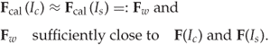
Both cover and stego estimates are intuitive to interpret and use for steganalysis. With cover estimates, ![]() for covers so any non-zero value indicates a steganogram. With stego estimates it is the other way around, and
for covers so any non-zero value indicates a steganogram. With stego estimates it is the other way around, and ![]() for steganograms.
for steganograms.
Kodovský and Fridrich (2009) also discuss other types of reference transforms. The simplest example is a parallel reference, where
![]()
for some constant ![]() . This is clearly degenerate, as it is easy to see that
. This is clearly degenerate, as it is easy to see that
![]()
so that the difference-calibrated feature vector contains no information about whether the image is a steganogram or not.
The eraser transform is in a sense similar to stego and cover transforms. The eraser aims to estimate some abstract point which represents the cover image, and which is constant regardless of whether the cover is clean or a message has been embedded. This leads to two requirements (Kodovský and Fridrich, 2009):
The second requirement is a bit loosely defined. The essence of it is that ![]() must depend on the image
must depend on the image ![]() /
/![]() . Requiring that the feature vector of the transform is ‘close’ to the feature vectors of
. Requiring that the feature vector of the transform is ‘close’ to the feature vectors of ![]() and
and ![]() is just one way of achieving this.
is just one way of achieving this.
Both stego and cover estimates result in very simple and intuitive classifiers. One class will have ![]() (or
(or ![]() ), and the other class will have something different. This simple classifier holds regardless of the relationship between
), and the other class will have something different. This simple classifier holds regardless of the relationship between ![]() and
and ![]() , as long as they are ‘sufficiently’ different. This is not the case with the eraser transform. For the eraser to provide a simple classifier, the shift
, as long as they are ‘sufficiently’ different. This is not the case with the eraser transform. For the eraser to provide a simple classifier, the shift ![]() caused by embedding must be consistent.
caused by embedding must be consistent.
The last class of reference transforms identified by Kodovský and Fridrich (2009) is the divergence transform, which serves to boost the difference between clean image and steganogram by pulling ![]() and
and ![]() in different directions. In other words,
in different directions. In other words, ![]() and
and ![]() , where
, where ![]() .
.
It is important to note that the concepts of cover and stego estimates are defined in terms of the feature space, whereas the reference transform operates in image space. We never assume that ![]() or
or ![]() ; we are only interested in the relationship between
; we are only interested in the relationship between ![]() and
and ![]() or
or ![]() . Therefore the same reference transform may be a good cover estimate with respect to one feature set, but degenerate to parallel reference with respect to another.
. Therefore the same reference transform may be a good cover estimate with respect to one feature set, but degenerate to parallel reference with respect to another.
9.5 Progressive Randomisation
Over-embedding with a new message has been used by several authors in non-learning, statistical steganalysis. Rocha (2006) also used it in the context of machine learning; see Rocha and Goldenstein (2010) for the most recent presentation of the work. They used six different calibrated images, over-embedding with six different embedding rates, namely
![]()
Each ![]() leads to a reference transform
leads to a reference transform ![]() by over-embedding with LSB at a rate
by over-embedding with LSB at a rate ![]() of capacity, forming a steganogram
of capacity, forming a steganogram ![]() .
.
Rocha used the reciprocal of the ratio-calibrated feature discussed earlier. That is, for each base feature ![]() , the calibrated feature is given as
, the calibrated feature is given as
![]()
where ![]() is the intercepted image.
is the intercepted image.
This calibration method mainly makes sense when we assume that intercepted steganograms will have been created with LSB embedding. In a sense, the reference transform ![]() will be a stego estimate with respect to any feature, but the hypothetical embedding rate in the stego estimate will not be constant. If we have an image of size
will be a stego estimate with respect to any feature, but the hypothetical embedding rate in the stego estimate will not be constant. If we have an image of size ![]() with
with ![]() bits embedded with LSB embedding, and we then over-embed with
bits embedded with LSB embedding, and we then over-embed with ![]() bits, the result is a steganogram with
bits, the result is a steganogram with ![]() embedded bits, where
embedded bits, where
9.6 ![]()
This can be seen because, on average, ![]() of the new bits will just overwrite parts of the original message, while
of the new bits will just overwrite parts of the original message, while ![]() bits will use previously unused capacity. Thus the calibration will estimate a steganogram at some embedding rate
bits will use previously unused capacity. Thus the calibration will estimate a steganogram at some embedding rate ![]() , but
, but ![]() depends not only on
depends not only on ![]() , but also on the message length already embedded in the intercepted image.
, but also on the message length already embedded in the intercepted image.
Looking at (9.6), we can see that over-embedding makes more of a difference to a natural image ![]() than to a steganogram
than to a steganogram ![]() . The difference is particularly significant if
. The difference is particularly significant if ![]() has been embedded at a high rate and the over-embedding will largely touch pixels already used for embedding.
has been embedded at a high rate and the over-embedding will largely touch pixels already used for embedding.
Even though Rocha did not use the terminology of calibration, their concept of progressive randomisation fits well in the framework. We note that the concept of a stego estimate is not as well-defined as we assumed in the previous section, because steganograms with different message lengths are very different. Apart from this, progressive randomisation is an example of a stego estimate. No analysis was made to decide which embedding rate ![]() gives the best reference transform
gives the best reference transform ![]() , leaving this problem instead for the learning classifier.
, leaving this problem instead for the learning classifier.
We will only give a brief summary of the other elements making up Rocha's feature vector. They used a method of dividing the image into sub-regions (possibly overlapping), calculating features from each region. Two different underlying features were used. The first one is the ![]() statistic which we discussed in Chapter 2. The second one is a new feature, using Maurer's (1992) method to measure the randomness of a bit string. Maurer's measure is well suited for bit-plane analysis following the ideas from Chapter 5. If we consider the LSB plane as a 1-D vector, it should be a random-looking bit sequence for a steganogram, and may or may not be random-looking for a clean image, and this is what Maurer's test is designed to detect.
statistic which we discussed in Chapter 2. The second one is a new feature, using Maurer's (1992) method to measure the randomness of a bit string. Maurer's measure is well suited for bit-plane analysis following the ideas from Chapter 5. If we consider the LSB plane as a 1-D vector, it should be a random-looking bit sequence for a steganogram, and may or may not be random-looking for a clean image, and this is what Maurer's test is designed to detect.