Chapter 10

Simulation and Evaluation

In Chapter 3 we gave a simple framework for testing and evaluating a classifier using accuracy, and with the subsequent chapters we have a sizeable toolbox of steganalysers. There is more to testing and evaluation than just accuracy and standard errors, and this chapter will dig into this problem in more depth. We will look at the simulation and evaluation methodology, and also at different performance heuristics which can give a more detailed picture than the accuracy does.

10.1 Estimation and Simulation

One of the great challenges of science and technology is incomplete information. Seeking knowledge and understanding, we continuously have to make inferences from a limited body of data. Evaluating a steganalyser, for instance, we desire information about the performance of the steganalyser on the complete population of images that we might need to test in the future. The best we can do is to select a sample (test set) of already known images to check. This sample is limited both by the availability of images and by the time available for testing.

Statistics is the discipline concerned with quantitative inferences drawn from incomplete data. We will discuss some of the basics of statistics while highlighting concepts of particular relevance. Special attention will be paid to the limitations of statistical inference, to enable us to take a critical view on the quantitative assessments which may be made of steganalytic systems. For a more comprehensive introduction to statistics, we recommend Bhattacharyya and Johnson (1977).

10.1.1 The Binomial Distribution

Let us start by formalising the concept of accuracy and the framework for estimating it. In testing a classifier, we are performing a series of independent experiments or trials. Each trial considers a single image, and it produces one out of two possible outcomes, namely success (meaning that the object was correctly classified) or failure (meaning that the object was misclassified).

Such experiments are known as Bernoulli trials, defined by three properties:

1. Each trial has two possible outcomes, often labelled ‘success’ () and ‘failure’ ().

2. Every trial in the series has the same probabilities and .

3. The trials are independent, so that the probabilities and are invariant, and do not change as a function of previous outcomes.

Evaluating a classifier according to the framework from Chapter 3, we are interested in the probability of success, or correct classification. Thus the accuracy is equal to the success probability, i.e. .

A Bernoulli trial can be any kind of independent trial with a binary outcome. The coin toss, which has ‘head’ () or ‘tail’ () as the two possible outcomes, is the fundamental textbook example. Clearly the probability is , unless the coin is bent or otherwise damaged. In fact, we tend to refer to any Bernoulli trial with as a coin toss. Other examples include:

• testing a certain medical drug on an individual and recording if the response is positive () or negative ();
• polling an individual citizen and recording if he is in favour of () or against () a closer fiscal union in the EU;
• polling an individual resident and recording whether he/she is unemployed () or not ();
• catching a salmon and recording whether it is infected with a particular parasite () or not ().

Running a series of Bernoulli trials and recording the number of successes gives rise to the binomial distribution. The stochastic variable can take any value in the range , and the probability that we get exactly successes is given as

and the expected number of successes is

The test phase in the development of a steganalyser is such a series of Bernoulli trials. With a test set of images, we expect to get correct classifications on average, but the outcome is random so we can get more and we can get less. Some types of images may be easier to classify than others, but since we do not know which ones are easy, this is just an indistinguishable part of the random process.

10.1.2 Probabilities and Sampling

Much of our interest centres around probabilities; the most important one so far being the accuracy, or probability of correct classification. We have used the word probability several times, relying on the user's intuitive grasp of the concept. An event which has a high probability is expected to happen often, while one with low probability is expected to be rare. In reality, however, probability is an unusually tricky term to define, and definitions will vary depending on whether you are a mathematician, statistician, philosopher, engineer or layman.

A common confusion is to mistake probabilities and rates. Consider some Bernoulli trial which is repeated times and let denote the number of successes. The success rate is defined as . In other words, the rate is the outcome of an experiment. Since is a random variable, we will most likely get a different value every time we run the experiment.

It is possible to interpret probability in terms of rates. The success probability can be said to be the hypothetical success rate one would get by running an infinite number of trials. In mathematical terms, we can say that

Infinity is obviously a point we will never reach, and thus no experiment will ever let us measure the exact probability. Statistics is necessary when we seek information about a population of objects which is so large that we cannot possibly inspect every object, be it infinite or large but finite. If we could inspect every object, we would merely count them, and we could measure precisely whatever we needed to know.

In steganalysis, the population of interest is the set of all images we might intercept. All the images that Alice sends and Wendy inspects are drawn randomly from according to some probability distribution , which depends on Alice's tastes and interests. The accuracy is the probability that the classifier will give the correct prediction when it is presented with an image drawn from .

Trying to estimate , or any other parameter of or , the best we can do is to study a sample . Every parameter of the population has an analogue parameter defined on the sample space. We have the population accuracy or true accuracy, and we have a sample accuracy that we used as an estimate for the population accuracy. We can define these parameters in terms of the sample and the population. Let be a steganalyser. For any image , we write for the predicted class of and for the true class. We can define the population accuracy as

where if the statement is true and otherwise. The sample accuracy is defined as

If the sample is representative for the probability distribution on the population, then . But here is one of the major open problems in steganalysis. We know almost nothing about what makes a representative sample of images. Making a representative sample in steganalysis is particularly hard because the probability distribution is under adversarial control. Alice can choose images which she knows to be hard to classify.

10.1.3 Monte Carlo Simulations

It would be useful if we could test the steganalyser in the field, using real steganograms exchanged between real adversaries. Unfortunately, it is difficult to get enough adversaries to volunteer for the experiment. The solution is to use simulations, where we aim to simulate, or mimic, Alice's behaviour.

Simulation is not a well-defined term, and it can refer to a range of activities and techniques with rather different goals. Our interest is in simulating random processes, so that we can synthesise a statistical sample for analysis. Instead of collecting real statistical data in the field, we generate pseudo-random data which just simulates the real data. This kind of simulation is known as Monte Carlo simulation, named in honour of classic applications in simulating games.

Our simulations have a lot in common with applications in communications theory and error control coding, where Monte Carlo simulations are well established and well understood as the principal technique to assess error probabilities (Jeruchim et al., 2000). The objective, both in error control coding and in steganalysis, is to estimate the error probability of a system, and we get the estimate by simulating the operating process and counting error events.

Monte Carlo simulations are designed to generate pseudo-random samples from some probability distribution, and this is commonly used to calculate statistics of the distribution. The probability distribution we are interested in is that of classification errors in the classifier, that is a distribution on the sample space , but without knowledge of the error probability we cannot sample it directly. What we can do is use Monte Carlo processes to generate input (images) for the classifier, run the classifier to predict a class label and then compare it to the true label. A sample Monte Carlo system is shown in Figure 10.1.

Figure 10.1 Monte Carlo simulator system for steganalysis. All the white boxes are either random processes or processes which we cannot model deterministically

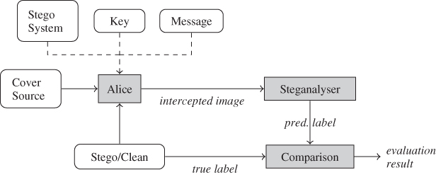
The input to the classifier is the product of several random processes, or unknown processes which can only be modelled as random processes. Each of those random processes poses a Monte Carlo problem; we need some way to generate pseudo-random samples. The key will usually be a random bit string, so that poses no challenge. The message would also need to be random or random-looking, assuming that Alice compresses and/or encrypts it, but the message length is not, and we know little about the distribution of message lengths. Then we have Alice's choice of whether to transmit a clean image or a steganogram, which gives rise to the class skew. This is another unknown parameter. The cover image comes from some cover source chosen by Alice, and different sources have different distributions.

The figure illustrates the limitations of straight-forward Monte Carlo simulations. We still have five input processes to simulate, and with the exception of the key, we have hardly any information about their distribution. By pseudo-randomly simulating the five input processes, for given message length, cover source, stego algorithm and class skew, Monte Carlo simulations can give us error probabilities for the assumed parameters. We would require real field data to learn anything about those input distributions, and no one has attempted that research yet.

10.1.4 Confidence Intervals

Confidence intervals provide a format to report estimates of some parameter , such as an accuracy or error probability. The confidence interval is a function of the observed data , and it has an associated confidence level . The popular, but ambiguous, interpretation is that the true value of is contained in the confidence interval with probability . Mathematically, we write it as

The problem with this interpretation is that it does not specify the probability distribution considered. The definition of a confidence interval is that the a priori probability of the confidence interval containing , when is drawn randomly from the appropriate probability distribution, is . Thus both and are considered as random variables.

A popular misconception occurs when the confidence interval is calculated for a given observation , and the confidence level is thought of as a posterior probability. The a posteriori probability

may or may not be approximately equal to the a priori probability . Very often the approximation is good enough, but for instance MacKay (2003) gives instructive examples to show that it is not true in general. In order to relate the confidence level to probabilities, it has to be in relation to the probability distribution of the observations .

The confidence interval is not unique; any interval which satisfies the probability requirement is a confidence interval. The most common way to calculate a confidence interval coincides with the definition of error bounds as introduced in Section 3.2. Given an estimator of , we define an error bound with confidence level as

where is the standard deviation of and is the point such that for a standard normally distributed variable . Quite clearly, satisfies the definition of a confidence interval with a confidence level of , if is normally distributed, which is the case if the underlying sample of observations is large according to the central limit theorem. In practice, we do not know , and replacing by some estimate, we get an approximate confidence interval.

Error bounds imply that some estimator has been calculated as well, so that the estimate is quoted with the bounds. A confidence interval, in contrast, is quoted without any associated estimator. Confidence intervals and error bounds can usually be interpreted in the same way. Confidence intervals provide a way to disclose the error bounds, without explicitly disclosing the estimator.

10.2 Scalar Measures

We are familiar with the accuracy and the error rate , as well as the empirical estimators. As a performance indicator, they are limited, and hide a lot of detail about the actual performance of our classifier. Our first step is to see that not all errors are equal.

10.2.1 Two Error Types

Presented with an image , our steganalyser will return a verdict of either ‘stego’ or ‘non-stego’. Thus we have two possible predicted labels, and also two possible true labels, for a total of four possible outcomes of the test, as shown in the so-called confusion matrix (Fawcett, 2006) in Figure 10.2. The columns represent what actually is, while the rows represent what the steganalyser thinks it is. Both the upper-right and lower-left cells are errors:

Figure 10.2 The confusion matrix

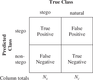
In many situations, these two error types may have different associated costs. Criminal justice, for instance, has a very low tolerance for accusing the innocent. In other words, the cost of false positives is considered to be very high compared to that of false negatives.

Let and denote the probability, respectively, of a false positive and a false negative. These are conditional probabilities

where and are, respectively, the set of all cover images and all steganograms. The detection probability , as a performance measure, is equivalent to the false negative probability, but is sometimes more convenient. As is customary in statistics, we will use the hat to denote empirical estimates. Thus, and denote the false positive and false negative rates, respectively, as calculated in the test phase.

The total error probability of the classifier is given as

10.1

In other words, the total error probability depends, in general, not only on the steganalyser, but also on the probability of intercepting a steganogram. This is known as the class skew. When nothing is known about the class skew, one typically assumes that there is none, i.e. . However, there is no reason to think that this would be the case in steganalysis.

Example 10.2.1

Provos and Honeyman (2003) ran an experiment to check if image steganography is in active use on eBay and on Usenet news. They used a web crawler to harvest images, and every image found was steganalysed. They found up to 2.1% positives (including false positives) testing for JP Hide on Usenet, and 1% on eBay. These rates are comparable to the false positive rates for the steganalyser, and thus the initial test gives no information as to whether steganography is being used.

In order to complete the test, they ran a secondary attack, consisting of dictionary attacks aiming to recover the password used by the stego-systems. Such password attacks are time-consuming, and thus constitute a cost of false positives. If the initial steganalyser has a high false positive rate, it will slow down the secondary attack before more candidate images must be tested.

In such a scientific experiment, where the aim was to verify or quantify the use of steganography in the wild, a high false negative rate is not an issue. Unless the number of steganograms in the sample set is negligibly small, we will find a certain number of steganograms, and if we multiply by we get a good estimate of the total number of steganograms. The FN rate just needs to be so low that we identify a statistically significant number of steganograms.

---

The examples are undoubtedly cases of extreme class skew. Most Internet users have probably not even heard of steganography, let alone considered using it. If, say, , it is trivial to make a classifier with error probability . We just hypothesise ‘non-stego’ regardless of the input, and we only have an error in the rare case that is a steganogram. In such a case, the combined error probability is irrelevant, and we would clearly want to estimate and separately.

10.2.2 Common Scalar Measures

Besides and , there is a large number of other measures which are used in the literature. It is useful to be aware of these, even though most of them depend very much on the class skew.

In practice, all measures are based on empirical statistics from the testing; i.e. we find distinct natural images, and create steganograms out of of them. We run the classifier on each image and count the numbers of false positives (), true positives (), false negatives () and true negatives (). Two popular performance indicators are the precision and the recall. We define them as follows:

The precision is the fraction of the predicted steganograms which are truly steganograms, whereas the recall is the number of actual steganograms which are correctly identified. Very often, a harmonic average of the precision and recall is used. This is defined as follows:

which can also be weighted by a constant . Both and are common:

Finally, we repeat the familiar accuracy:

which is the probability of correct classification. Of all of these measures, only the recall is robust to class skew. All the others use numbers from both columns in the confusion matrix, and therefore they will change when we change the class sizes and relative to each other.

10.3 The Receiver Operating Curve

So far we have discussed the evaluation of discrete classifiers which make a hard decision about the class prediction. Many classifiers return or can return soft information, in terms of a classification score for any object (image) . The hard decision classifier will then consist of two components; a model, or heuristic function which returns the classification score, and a threshold . The hard decision rule assigns one class for and the other for . Classification scores close to the threshold indicate doubt. If is large, the class prediction can be made with confidence.

The threshold can be varied to control the trade-off between the false negative rate and the false positive rate . When we move the threshold, one will increase and the other will decrease. This means that a soft decision classifier defined by leaves us some flexibility, and we can adjust the error rates by varying the threshold. How can we evaluate just the model universally, without fixing the threshold?

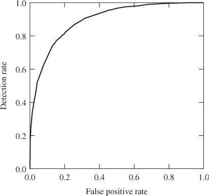
Figure 10.3 shows an example of the trade-off controlled by the threshold . We have plotted the detection rate on the -axis and the false positive rate on the -axis. Every point on the curve is a feasible point, by choosing a suitable threshold. Thus we can freely choose the false positive rate, and the curve tells us the resulting detection rate, or vice versa. This curve is known as the receiver operating characteristic (ROC). We will discuss it further below, starting with how to calculate it empirically.

Figure 10.3 Sample ROC curves for the PEV-219 feature vector against 512 bytes F5 embedding. The test set is the same as the one used in Chapter 8

10.3.1 The libSVM API for Python

Although the command line tools include everything that is needed to train and test a classifier, more advanced analysis is easier by calling libSVM through a general-purpose programming language. The libSVM distribution includes two SVM modules, svm and svmutil.

train   = svm.svm_problem( labels1, fvectors1 )
param   = svm.svm_parameter( )
model   = svmutil.svm_train( dataset, param )
(L,A,V) = svmutil.svm_predict( labels2, fvectors2, model )

Code Example 10.1 shows how training and testing of an SVM classifier can be done within Python. The output is a tuple . We will ignore , which includes accuracy and other performance measures. Our main interest is the list of classification scores, . The list of predicted labels is calculated from , with a threshold . Thus a negative classification score represents one class, and a positive score the other.

It may be instructive to see the classification scores visualised as a histogram. Figure 10.4 gives an example of classification scores from two different classifiers using Shi et al.'s Markov features. Steganograms (black) and natural images (grey) are plotted separately in the histogram. A threshold is chosen as a point on the -axis, so that scores to the left will be interpreted as negatives (natural image) and scores to the right as positives (steganograms). Grey bars to the right of the threshold point are false positives, while black bars to the left are false negatives.

Figure 10.4 Distribution of classification scores for an SVM steganalyser using Shi et al.'s Markov model features: (a) default libSVM parameters; (b) optimised SVM parameters

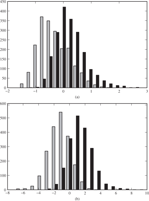
Clearly, we have a trade-off between false positives and false negatives. The further to the left we place our threshold, the more positives will be hypothesised. This results in more detections, and thus a lower false negative rate, but it also gives more false positives. Comparing the two histograms in Figure 10.4(b), it is fairly easy to choose a good threshold, almost separating the steganograms from the natural images. The steganalyser with default parameters has poor separation. Regardless of where we place the threshold, there will be a lot of instances on the wrong side. In this case the trade-off is very important, and we need to prioritise between the two error rates.

Code Example 10.2 : Generating the ROC plot in Python. The input parameters are a list of classification labels () Y and a list of classification scores V

def rocplot(Y,V):
   V1 = [ V[i] for i in range(len(V)) if Y[i] == −1 ]
   V2 = [ V[i] for i in range(len(V)) if Y[i] == +1 ]
   (mn,mx) = ( min(V), max(V) )
   bins = [ mn + (mx−mn)*i/250 for i in range(251) ]
   (H1,b) = np.histogram( V1, bins )
   (H2,b) = np.histogram( V2, bins )
   H1 = np.cumsum( H1.astype( float ) ) / len(V1)
   H2 = np.cumsum( H2.astype( float ) ) / len(V2)
   matplotlib.pyplot.plot( H1, H2 )

---

The ROC curve is also a visualisation of the classification scores. Let and be the sets of classification scores in testing of clean images and steganograms, respectively. We calculate the relative, cumulative histograms

The ROC plot is then defined by plotting the points for varying values of . Thus each point on the curve represents some threshold value , and it displays the two corresponding probability estimates and on the respective axes. Code Example 10.2 illustrates the algorithm in Python.

It may be necessary to tune the bin boundaries to make a smooth plot. Some authors suggest a more brute-force approach to create the ROC plot. In our code example, we generate 250 points on the curve. Fawcett (2006) generates one plot point for every distinct classification score present in the training set. The latter approach will clearly give the smoothest curve possible, but it causes a problem with vector graphics output (e.g. PDF) when the training set is large, as every point has to be stored in the graphics file. Code Example 10.2 is faster, which hardly matters since the generation of the data set Y and V would dominate, and more importantly, the PDF output is manageable regardless of the length of V.

10.3.2 The ROC Curve

The ROC curve visualises the trade-off between detection rate and false positives. By changing the classification threshold, we can move up and down the curve. Lowering the threshold will lead to more positive classifications, both increasing the detection (true positives) and false positives alike.

ROC stands for ‘receiver operating characteristic’, emphasising its origin in communications research. The acronym is widely used within different domains, and the origin in communications is not always relevant to the context. It is not unusual to see the C interpreted as ‘curve’. The application of ROC curves in machine learning can be traced back at least to Swets (1988) and Spackman (1989), but it has seen an increasing popularity in the last decade. Ker (2004b) interpreted ROC as region of confidence, which may be a more meaningful term in our applications. The region under the ROC curve describes the confidence we draw from the classifier.

The ROC space represents every possible combination of FP and TP probabilities. Every discrete classifier corresponds to a point in the ROC space. The perfect, infallible classifier would be at the point . A classifier which always returns ‘stego’ regardless of the input would sit at , and one which always returns ‘clean’ at .

The diagonal line, from to , corresponds to some naïve classifier which returns ‘stego’ with a certain probability independently of the input. This is the worst possible steganalyser. If we had a classifier operating under the main diagonal, i.e. where , we could easily convert it into a better classifier . We would simply run and let return ‘stego’ if returns ‘non-stego’ and vice versa. The resulting error probabilities and of would be given as

This conversion reflects any point on the ROC curve around the main diagonal and allows us to assume that any classifier should be above the main diagonal.

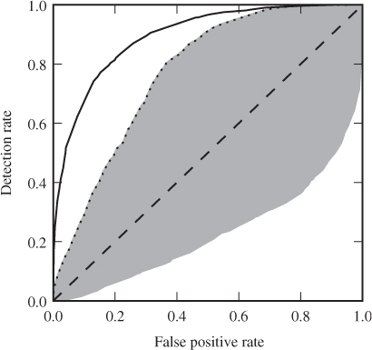
This is illustrated in Figure 10.5, where the worthless classifier is shown as the dashed line. Two classifiers, with and without grid search, are compared, and we clearly see that the one with grid search is superior for all values. We have also shown the reflection of the inferior ROC curve around the diagonal. The size of the grey area can be seen as its improvement over the worthless classifier.

Figure 10.5 Sample ROC curves for the PEV-219 feature vector against 512 bytes F5 embedding. The test set is the same as the one used in Chapter 8. The upper curve is from libSVM with grid search optimised parameters, whereas the lower curve is for default parameters. The shaded area represents the Giri coefficient of the non-optimised steganalyser. The features have been scaled in both cases

Where discrete classifiers correspond to a point in ROC space, classifiers with soft output, such as SVM, correspond to a curve. Every threshold corresponds to a point in ROC space, so varying the threshold will draw a curve, from corresponding to a threshold of to which corresponds to a threshold of .

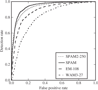
The ROC curve for a soft output classifier is good at visualising the performance independently of the selected threshold. Figure 10.6 shows an example comparing different feature vectors. As we can see, we cannot consistently rank them based on the ROC curve. Two of the curves cross, so that different feature vectors excel at different FP probabilities. Which feature vector we prefer may depend on the use case.

Figure 10.6 ROC plot comparing different feature vectors on a 10% LSB embedding

One of the important properties of the ROC curve is that it is invariant irrespective of class skew. This follows because it is the collection of just feasible points , and both and measure the performance for a single class of classifier input and consequently are invariant. We also note that classification scores are considered only as ordinal measures, that is, they rank objects in order of how plausibly they could be steganograms. The numerical values of the classification scores are irrelevant to the ROC plots, and thus we can compare ROC plots of different classifiers even if the classification scores are not comparable. This is important as it allows us to construct ROC plots for arbitrary classifier functions without converting the scores into some common scale such as likelihoods or -values. Any score which defines the same order will do.

10.3.3 Choosing a Point on the ROC Curve

There is a natural desire to search for one scalar heuristic to rank all classifiers according to their performance. What the ROC plot tells us is that there is no one such scalar. In Figure 10.6 we clearly see that one classifier may be superior at one point and inferior at another. Every point on the curve matters. Yet sometimes we need a scalar, and different authors have selected different points on the ROC curve for comparison. The following suggestions have been seen in the steganalysis literature, each with good theoretical reasons (Westfeld, 2007):

1. Fix , and use this combined error probability as the performance heuristic.

2. Fix , and use as the heuristic.

3. Fix , and use as the heuristic.

Using equal error rates is very common in for instance biometrics, and has the advantage that the total error probability in (10.1) becomes independent of class skew.

Aiming at a low false positive probability is natural when one targets applications where it is more serious to falsely accuse the innocent than fail to detect the guilty, which is the case in criminal law in most countries. Some early papers in steganalysis used zero false positives as their target point on the ROC curve. This would of course be great, with all innocent users being safe, if we could calculate it, but it is infeasible for two reasons. From a practical viewpoint, we should long have realised that no system is perfect, so even though we can get arbitrarily close to zero, we will never get equality. The theoretical viewpoint is even more absolute. Estimating probabilities close to 0 requires very large samples. As the probability to be estimated tends to zero, the required sample size will tend to infinity. The chosen point on the ROC curve has to be one which can be estimated with a reasonably small error bound. Using is quite arbitrary, but it is a reasonable trade-off between low FP probability and feasibility of estimation.

The last proposal, with , advocated by Ker (2004a), may sound strange. Intuitively, we may find 50% detection unacceptable for most applications. However, if the secret communications extend over time, and the steganalyst acts repeatedly, the steganography will eventually be detected. The advantage of is that the threshold is then equal to the median of the classifier soft output for steganograms, at which point the detection probability is independent of the variance of . This removes one unknown from the analysis, and less information is required about the statistical properties of steganograms.

10.3.4 Confidence and Variance

The ROC curves we learnt to draw in Section 10.3.1 are mere snapshots of performance on one single test set, just as a single observation of the sample accuracy would be. There has been a tendency in the machine learning literature to overstate observations from such ROC plots (Fawcett, 2003), by treating better as better without distinguishing between approximately equal and significantly better. In order to make confident conclusions, we need a notion of standard errors or confidence intervals.

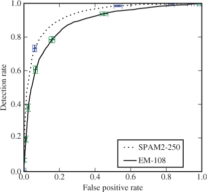
Variance and confidence intervals are defined for scalar points, and there is no one canonical way to generalise it for curves. However, since each point visualises two scalars, and , we can calculate confidence intervals or error bounds along each of the axes. This is shown in Figure 10.7, where the vertical and horizontal bars show a error bound for and respectively. The error bounds are calculated using the standard estimator for the standard error of the binomial parameter, namely

Figure 10.7 Example of ROC plot marking confidence intervals for and for some thresholds

where is the sample size. Note that there is no correspondence between points on the different curves. Each point corresponds to a given classifier threshold, but since classification scores are not comparable between different soft output classifiers, the thresholds are not comparable either.

In the example, we can observe that the confidence intervals are narrow and are far from reaching the other curve except for error rates close to . This method of plotting error bars gives a quick and visual impression of the accuracy of the ROC plot, and is well worth including.

Several authors have studied confidence intervals for ROC curves, and many methods exist. Fawcett (2003) gives a broad discussion of the problem, and the importance of considering the variance. Macskassy and Provost (2004) discuss methods to calculate confidence bands for the ROC curve. It is common to use cross-validation or bootstrapping to generate multiple ROC curves, rather than the simple method we described above, but further survey or details on this topic is beyond the scope of this book.

10.3.5 The Area Under the Curve

There is one well-known alternative to picking a single point on the ROC curve, namely measuring the area under the curve (AUC), that is, integrate the ROC curve on the interval :

where we consider as a function of , as visualised by the ROC curve. The worst possible classifier, namely the random guessing represented by a straight line ROC curve from to , has an AUC of . No realistic classifier should be worse than this. Hence the AUC has range to .

It may seem more natural to scale the heuristic so that the worst possible classifier gets a value of 0. A popular choice is the so-called Gini coefficient (Fawcett, 2003), which is equivalent to the reliability that Fridrich (2005) defined in the context of steganalysis. The Gini coefficient can be defined as

The measure corresponds to the shaded area in Figure 10.5. Clearly, the perfect classifier has and random guessing has .

The AUC also has another important statistical property. If we draw a random steganogram and a random clean image , and let and denote their respective classification scores, then

In other words, the AUC gives us the probability of correct pairwise ranking of objects from different classes.

Westfeld (2007) compared the stability of the four scalar heuristics we have discussed, that is, he sought the measure with the lowest variation when the same simulation is repeated. He used synthetic data to simulate the soft output from the classifier, assuming either Gaussian or Cauchy distribution. He used 1000 samples each for stego and non-stego, and repeated the experiment to produce 100 000 ROC curves. Westfeld concluded that the error rate at equal error rates and the Gini coefficient were very close in stability, with being the most stable for Cauchy distribution and being the most stable for Gaussian distribution. The false positive rate at 50% detection () was only slightly inferior to the first two. However, the detection rate at false positives was significantly less stable. This observation is confirmed by our Figure 10.7, where we can see a high variance for the detection rate at low false positive rates, and a low variance for when the detection rate is high.

Code Example 10.3 : Calculating the AUC. The input parameters are lists of the and coordinates of the points on the curve, that is the H1 and H2 variables calculated in Code Example 10.2

def auc(H1,H2):
   heights = [ (a+b)/2 for (a,b) in zip(H1[1:],H1[:−1]) ]
   widths  = [ (a−b) for (a,b) in zip(H2[1:],H2[:−1]) ]
   areas   = [ h*w for (h,w) in zip(heights,widths) ]
   return sum(areas)

---

The AUC can be calculated using the trapezoidal rule for numerical integration. For each pair of adjacent points on the ROC curve, and , we calculate the area of the trapezoid with corners at , , , . The area under the curve is (roughly) made up of all the disjoint trapezoids for , and we simply add them together. This is shown in Code Example 10.3.

10.4 Experimental Methodology

Experiments with machine learning can easily turn into a massive data management problem. Evaluating a single feature vector, a single stego-system and one cover source is straight forward and gives little reason to think about methodology. A couple of cases can be done one by one manually, but once one starts to vary the cover source, the stego-system, the message length and introduce numerous variations over the feature vectors, manual work is both tedious and error-prone. There are many tests to be performed, reusing the same data in different combinations. A robust and systematic framework to generate, store, and manage the many data sets is required.

Feature extraction is the most time-consuming part of the job, and we clearly do not want to redo it unnecessarily. Thus, a good infrastructure for performing the feature extraction and storing feature data is essential. This is a complex problem, and very few authors have addressed it. Below, we will discuss the most important challenges and some of the solutions which have been reported in the literature.

10.4.1 Feature Storage

The first question is how to store the feature vectors. The most common approach is to use text files, like the sparse format used by the libSVM command line tools. Text files are easy to process and portable between programs. However, text files easily become cumbersome when one takes an interest in individual features and sets out to test variations of feature vectors. Normally, one will only be able to refer to an individual feature by its index, which may change when new features are added to the system, and it is easy to get confused about which index refers to which feature. A data structure that can capture metadata and give easy access to sub-vectors and individual features is therefore useful.

In the experiments conducted in preparation for this book, the features were stored as Python objects, which were stored in binary files using the pickle module. This solution is also very simple to program, and the class can be furnished with any kind of useful metadata, including names and descriptions of individual features. It is relatively straight forward to support extraction of sub-vectors. Thus one object can contain all known features, and the different feature vectors of interest can be extracted when needed.

There are problems with this approach. Firstly, data objects which are serialised and stored using standard libraries, like pickle, will often give very large files, and even though disk space is cheap, reading and writing to such files may be slow. Secondly, when new features are added to the system, all the files need to be regenerated.

Ker (2004b) proposed a more refined and flexible solution. He built a framework using an SQL database to store all the features. This would tend to take more time and/or skill to program, but gives the same flexibility as the Python objects, and on top of that, it scales better. Ker indicated that more than several hundred million feature vector calculations were expected. Such a full-scale database solution also makes it easy to add additional information about the different objects, and one can quickly identify missing feature vectors and have them calculated.

It may be necessary to store the seeds used for the pseudo-random number generators, to be able to reproduce every object of a simulation exactly. It is clearly preferable to store just the seeds that are used to generate random keys and random messages, rather than storing every steganogram, because the image data would rapidly grow out of hand when the experiments are varied.

10.4.2 Parallel Computation

The feature extraction in the tests we made for Chapters 4–9 took about two minutes per spatial image and more for JPEG. With 5000 images, this means close to a CPU week and upwards. Admittedly, the code could be made more efficient, but programmer time is more expensive than CPU time. The solution is to parallellise the computation and use more CPUs to reduce the running time.

Computer jobs can be parallellised in many different ways, but it always breaks down to one general principle. The work has to be broken into small chunks, so that multiple chunks can be done independently on different CPU cores. Many chunks will depend on others and will only be able to start when they have received data from other, completed chunks. The differences between paradigms stem from differences in the chunk sizes and the amount of data which must be exchanged when each parallel set of chunks is complete.

For a steganalysis system, a chunk could be the feature extraction from one image. The chunks are clearly independent, so there is no problem in doing them in parallel, and we are unlikely to have more CPU cores than images, so there is no gain in breaking the problem into smaller chunks. This makes parallelism very simple. We can just run each feature extraction as an independent process, dumping the result to file. Thus the computation can easily be distributed over a large network of computers. Results can be accumulated either by using a networked file system, or by connecting to a central database server to record them.

The simplest way to run a large series of jobs on multiple computers is to use a batch queuing system like PBS, Torque or condor. The different jobs, one feature extraction job per image for instance, can be generated and submitted, and the system will distribute the work between computers so that the load is optimally balanced. Batch queue systems are most commonly found on clusters and supercomputers tailored for number crunching, but they can also run on heterogeneous networks. It is quite feasible to install a batch queue system in a student lab or office network to take advantage of idle time out of hours.

There may be good reasons to create a special-purpose queuing system for complex experiments. This can be done using a client–server model, where the server keeps track of which images have been processed and the clients prompt the server for parameters to perform feature extraction. Ker (2004b) recommended a system in which queued jobs were stored in the same MySQL database where the results were stored. This has the obvious advantage that the same system is used to identify missing data and to queue the jobs to generate them.

It is quite fortunate that feature extraction is both the most time-consuming part of the experiment and also simple to parallellise across independent processes. Thus, most of the reward can be reaped with the above simple steps. It is possible to parallellise other parts of the system, but it may require more fine-grained parallelism, using either shared memory (e.g. open-MP) or message passing (e.g. MPI). Individual matrix operations may be speeded up by running constituent scalar operations in parallel, and this would allow us both to speed up feature extractions for one individual image for faster interactive use, and also to speed up SVM or other classifiers. Unless one can find a ready-made parallel-processing API to do the job, this will be costly in man hours, but when even laptop CPUs have four cores or more, this might be the way the world is heading. It can be very useful to speed up interactive trial and error exercises.

Not all programming languages are equally suitable for parallellisation. The C implementation of Python currently employs a global interpreter lock (GIL) which ensures that computation cannot be parallellised. The justification for GIL is that it avoids the overhead of preventing parallel code segments from accessing the same memory. The Java implementation, Jython, does not have this limitation, but then it does not have the same libraries, such as numpy.

10.4.3 The Dangers of Large-scale Experiments

There are some serious pitfalls when one relies on complex series of experiments. Most importantly, running enough experiments you will always get some interesting, surprising – and false – results. Consider, for instance, the simple case of estimating the accuracy, where we chose to quote twice the standard error to get error bounds. Running one test, we feel rather confident that the true accuracy will be within the bound, and in low-risk applications this is quite justified.

However, if we run 20 tests, we would expect to miss the error bound almost once on average. Running a thousand tests we should miss the error bound 46 times on average. Most of them will be a little off, but on average one will fall outside three times the standard error. Even more extreme results exist, and if we run thousands of tests looking for a surprising result, we will find it, even if no such result is correct. When many tests are performed in the preparation of analysis, one may require a higher level of confidence in each test. Alternatively, one can confirm results of particular interest by running additional experiments using a larger sample.

The discussion above, of course, implicitly assumes that the tests are independent. In practice, we would typically reuse the same image database for many tests, creating dependencies between the tests. The dependencies will make the analysis less transparent. Quite possibly, there are enough independent random elements to make the analysis correct. Alternatively, it is possible that extreme results will not occur as often, but in larger number when they occur at all.

To conclude, when large suites of experiments are used, care must be taken to ensure the level of confidence. The safest simple rule of thumb is probably to validate surprising results with extra, independent tests with a high significance level.

10.5 Comparison and Hypothesis Testing

In Chapter 3 we gave some rough guidelines on how much different two empirical accuracies had to be in order to be considered different. We suggested that accuracies within two standard errors of each other should be considered (approximately) equal.

A more formal framework to compare two classifiers would be to use a statistical hypothesis test. We remember that we also encountered hypothesis testing for the pairs-of-values test in Chapter 2, and it has been used in other statistical steganalysers as well. It is in fact quite common and natural to phrase the steganalysis problem as a statistical hypothesis test. In short, there are many good reasons to spend some time on hypothesis testing as a methodology.

10.5.1 The Hypothesis Test

A common question to ask in steganalysis research is this: Does steganalyser have a better accuracy than steganalyser ? This is a question which is well suited for a hypothesis test. We have two hypotheses:

where and denote the accuracy of steganalyser and respectively. Very often the experimenter hopes to demonstrate that a new algorithm is better than the current state of the art. Thus represents the default or negative outcome, while denotes, in a sense, the desired or positive outcome. The hypothesis is known as the null hypothesis.

Statistical hypothesis tests are designed to give good control of the probability of a false positive. We want to ensure that the evidence is solid before we promote the new algorithm. Hence, we require a known probability model under the condition that is true, so that we can calculate the probability of getting a result leading us to reject when we should not. It is less important to have a known probability model under , although we would need it if we also want to calculate the false negative probability.

The test is designed ahead of time, before we look at the data, in such a way that the probability of falsely rejecting is bounded. The test is staged as a contest between the two hypotheses, with clearly defined rules. Once the contest is started there is no further room for reasoning or discussion. The winning hypothesis is declared according to the rules.

In order to test the hypothesis, we need some observable random variable which will have different distributions under and . Usually, that is an estimator for the parameters which occur in the hypothesis statements. In our case the hypothesis concerns the accuracies and , and we will observe the empirical accuracies and . If , then is plausible. If , it is reasonable to reject . The question is, how much larger ought to be before we can conclude that is a better steganalyser?

10.5.2 Comparing Two Binomial Proportions

The accuracy is the success probability of a Bernoulli trial in the binomial distribution, also known as the binomial proportion. There is a standard test to compare the proportions of two different binomial distributions, such as for two different classifiers and . To formulate the test, we rephrase the null hypothesis as

Thus we can consider the single random variable , rather than two variables.

If the training set is at least moderately large, then is approximately normally distributed. The expectation and variance of are given as follows:

which can be estimated as

Thus we have a known probability distribution under , as required. Under we expect , while any large value of indicates that is less plausible. For instance, we know that the probability . In other words, if we decide to reject if , we know that the probability of making a false positive is less than . The probability of falsely rejecting the null hypothesis is known as the significance level of the hypothesis test, and it is the principal measure of the reliability of the test.

We can transform the random variable to a variable with standard normal distribution under , by dividing by the standard deviation. We define

10.2

which has zero mean and unit variance under the null hypothesis. The standard normal distribution makes the observed variable easier to handle, as it can be compared directly to tables for the normal distribution.

So far we have focused on the null hypothesis , and its negation has implicitly become the alternative hypothesis:

This hypothesis makes no statement as to which of or might be the better, and we will reject regardless of which algorithm is better, as long as they do not have similar performance.

Very often, we want to demonstrate that a novel classifier is superior to an established classifier . If , it may be evidence that is implausible, but it hardly proves the point we want to make. In such a case, the alternative hypothesis should naturally be

Which alternative hypothesis we make has an impact on the decision criterion. We discussed earlier that in a test of against at a significance level of , we would reject the null hypothesis if . If we test against however, we do not reject the null hypothesis for . At a significance level of we should reject if , since .

Example 10.5.1

Suppose we want to check if Cartesian calibration as discussed in Chapter 9 improves the performance of the Pevný features. That is, we want to compare CCPEV-438 (classifier X) with NCPEV-219 (classifier Y). The hypotheses are given as

We observe the random variable as defined in (10.2). Let's choose a significance level of and test the algorithms on a sample of 4000 images. The experiment returns and , and we calculate

We can look up the value such that for a normally distributed variable in Python:

In [34]: import scipy.stats

In [35]: N = scipy.stats.norm()

In [36]: N.ppf( [ 0.95 ] )
Out[36]: array([ 1.64485363])

---

Here N is defined as a standard normal distribution and ppf() is the inverse cumulative density function. Thus , and we can reject at significance. We conclude that Cartesian calibration improves the Pevný features.

10.6 Summary

A much too frequent pitfall in steganalysis is to exaggerate conclusions based on very simplified heuristics. It would be useful to re-evaluate many well-known stego-systems, aiming to get a more balanced, complete and confident assessment. Most importantly, a notion of confidence, or statistical significance, is required. This is well understood in statistics, and in many disciplines it would be unheard of to publish results without an assessment of error bounds and significance. In steganalysis there are still open problems to answer, where the original authors have cut corners.

Furthermore one needs to be aware that different applications will require different trade-offs between false positives and false negatives, and knowledge of the full ROC curve is often necessary. We also know that classifier performance will vary depending on message lengths and cover sources. To get a good picture of field performance, more than just a few combinations must be tried. We will return to these questions in Chapter 14.