
Chapter 11
Support Vector Machines
Support vector machines (SVM) are a good algorithm for starters who enter the field of machine learning from an applied angle. As we have demonstrated in previous chapters, easy-to-use software will usually give good classification performance without any tedious parameter tuning. Thus all the effort can be put into the development of new features.
In this chapter, we will investigate the SVM algorithm in more depth, both to extend it to one-class and multi-class classification, and to cover the various components that can be generalised. In principle, SVM is a linear classifier, so we will start by exploring linear classifiers in general. The trick used to classify non-linear problems is the so-called kernel trick, which essentially maps the feature vectors into a higher-dimensional space where the problem becomes linear. This kernel trick is the second key component, which can generalise to other algorithms.
11.1 Linear Classifiers
An object i is characterised by two quantities, a feature vector ![]() which can be observed, and a class label yi ∈ { − 1, + 1} which cannot normally be observed, but which we attempt to deduce from the observed
which can be observed, and a class label yi ∈ { − 1, + 1} which cannot normally be observed, but which we attempt to deduce from the observed ![]() . Thus we have two sets of points in n-space, namely
. Thus we have two sets of points in n-space, namely ![]() and
and ![]() , as illustrated in Figure 11.1. Classification aims to separate these two sets geometrically in
, as illustrated in Figure 11.1. Classification aims to separate these two sets geometrically in ![]() .
.
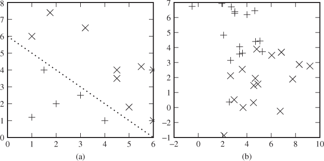
Figure 11.1 Feature vectors visualised in ![]() : (a) linearly separable problem; (b) linearly non-separable problem
: (a) linearly separable problem; (b) linearly non-separable problem
A linear classifier aims to separate the classes by drawing a hyperplane between them. In ![]() a hyperplane is a line, in
a hyperplane is a line, in ![]() it is a plane and in
it is a plane and in ![]() it is a subspace of dimension n − 1. If the problem is linearly separable, as it is in Figure 11.1(a), it is possible to draw such a hyperplane which cleanly splits the objects into two sets exactly matching the two classes. If the problem is not linearly separable, as in Figure 11.1(b), this is not possible, and any linear classifier will make errors.
it is a subspace of dimension n − 1. If the problem is linearly separable, as it is in Figure 11.1(a), it is possible to draw such a hyperplane which cleanly splits the objects into two sets exactly matching the two classes. If the problem is not linearly separable, as in Figure 11.1(b), this is not possible, and any linear classifier will make errors.
Mathematically, a hyperplane is defined as the set ![]() , for some vector
, for some vector ![]() , orthogonal on the hyperplane, and scalar w0. Using the hyperplane as a classifier is straightforward. The function
, orthogonal on the hyperplane, and scalar w0. Using the hyperplane as a classifier is straightforward. The function ![]() will be used as a classification heuristic. We have
will be used as a classification heuristic. We have ![]() on one side of the hyperplane and
on one side of the hyperplane and ![]() on the other, so simply associate the class labels with the sign of
on the other, so simply associate the class labels with the sign of ![]() . Let yi and
. Let yi and ![]() denote the labels and feature vectors used to calculate the function h( · ) during the training phase.
denote the labels and feature vectors used to calculate the function h( · ) during the training phase.
11.1.1 Linearly Separable Problems
The challenge is to find ![]() to define the hyperplane which gives the best possible classification; but what do we mean by ‘best’? Consider the example in Figure 11.2. Which of the two proposed classification lines is the better one?
to define the hyperplane which gives the best possible classification; but what do we mean by ‘best’? Consider the example in Figure 11.2. Which of the two proposed classification lines is the better one?
Figure 11.2 Two different classification hyperplanes for the same separable problem
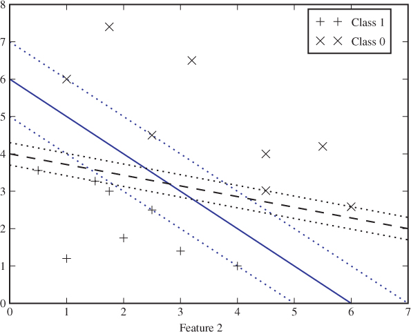
The solid line has a greater distance to the closest feature vector than the dashed line. We call this distance the margin of the classifier. Intuitively, it sounds like a good idea to maximise this margin. Remembering that the training points are only a random sample, we know that future test objects will be scattered randomly around. They are likely to be relatively close to the training points, but some must be expected to lie closer to the classifier line. The greater the margin, the less likely it is that a random point will fall on the wrong side of the classifier line.
We define two boundary hyperplanes parallel to and on either side of the classification hyperplane. The distance between the boundary hyperplane and the classification hyperplane is equal to the margin. Thus, there is no training point between the two boundary hyperplanes in the linearly separable case.
Consider a point ![]() and the closest point
and the closest point ![]() on the classification hyperplane. It is known that the distance
on the classification hyperplane. It is known that the distance ![]() between
between ![]() and the hyperplane is given as
and the hyperplane is given as
![]()
where the first equality is a standard observation of vector algebra.
It is customary to scale ![]() and w0 so that
and w0 so that ![]() for any point
for any point ![]() on the boundary hyperplanes. The margin is given as
on the boundary hyperplanes. The margin is given as ![]() for an arbitrary point
for an arbitrary point ![]() on the boundary hyperplanes and its closest point
on the boundary hyperplanes and its closest point ![]() on the classification hyperplane. Hence, with scaling, the margin is given as
on the classification hyperplane. Hence, with scaling, the margin is given as
![]()
To achieve maximum M, we have to minimise ![]() , that is, we want to solve
, that is, we want to solve
11.1 ![]()
11.2 ![]()
This is a standard quadratic optimisation problem with linear inequality constraints. It is a convex minimisation problem because J is a convex function, meaning that for any ![]() and any
and any ![]() , we have
, we have
![]()
Such convex minimisation problems can be solved using standard techniques based on the Lagrangian function ![]() , which is found by adding the cost function J and each of the constraints multiplied by a so-called Lagrange multiplier λi. The Lagrangian corresponding to J is given as
, which is found by adding the cost function J and each of the constraints multiplied by a so-called Lagrange multiplier λi. The Lagrangian corresponding to J is given as
where λi ≥ 0. It can be shown that any solution of (11.1) will have to be a critical point of the Lagrangian, that is a point where all the derivatives vanish:
11.3 ![]()
11.4 
11.5 ![]()
11.6 ![]()
These conditions are known as the Kuhn–Tucker or Karush–Kuhn–Tucker conditions. The minimisation problem can be solved by solving an equivalent problem, the so-called Wolfe dual representation, defined as follows:
![]()
subject to conditions (11.3) to (11.6), which are equivalent to
11.7 
11.8 
11.9 ![]()
Substituting for (11.7) and (11.8) in the definition of ![]() lets us simplify the problem to
lets us simplify the problem to
11.10 
subject to (11.8) and (11.9). Note that the only unknowns are now λi. The problem can be solved using any standard software for convex optimisation, such as CVXOPT for Python. Once (11.10) has been solved for the λi, we can substitute back into (11.7) to get ![]() . Finally, w0 can be found from (11.5).
. Finally, w0 can be found from (11.5).
The Lagrange multipliers λi are sometimes known as shadow costs, because each represents the cost of obeying one of the constraints. When the constraint is passive, that is satisfied with inequality, λi = 0 because the constraint does not prohibit a solution which would otherwise be more optimal. If, however, the constraint is active, by being met with equality, we get λi > 0 and the term contributes to increasing ![]() , imposing a cost on violating the constraint to seek a better solution. In a sense, we imagine that we are allowed to violate the constraint, but the cost λ does not make it worth while.
, imposing a cost on violating the constraint to seek a better solution. In a sense, we imagine that we are allowed to violate the constraint, but the cost λ does not make it worth while.
The formulation (11.10) demonstrates two key points of SVM. When we maximise (11.10), the second term will vanish for many (i, j) where λi = 0 or λj = 0. A particular training vector ![]() will only appear in the formula for
will only appear in the formula for ![]() if λi = 0, which means that
if λi = 0, which means that ![]() is on the boundary hyperplane. These training vectors are called support vectors.
is on the boundary hyperplane. These training vectors are called support vectors.
The second key point observed in (11.10) is that the feature vectors ![]() enter the problem in pairs, and only as pairs, as the inner product
enter the problem in pairs, and only as pairs, as the inner product ![]() . In particular, the dimensionality does not contribute explicitly to the cost function. We will use this observation when we introduce the kernel trick later.
. In particular, the dimensionality does not contribute explicitly to the cost function. We will use this observation when we introduce the kernel trick later.
11.1.2 Non-separable Problems
In most cases, the two classes are not separable. For instance, in Figure 11.1(b) it is impossible to draw a straight line separating the two classes. No matter how we draw the line, we will have to accept a number of classification errors, even in the training set. In the separable case we used the margin as the criterion for choosing the classification hyperplane. In the non-separable case we will have to consider the number of classification errors and possibly also the size (or seriousness) of each error.
Fisher Linear Discriminant
The Fisher linear discriminant (FLD) (Fisher, 1936) is the classic among classification algorithms. Without diminishing its theoretical and practical usefulness, it is not always counted as a learning algorithm, as it relies purely on conventional theory of statistics.
The feature vectors ![]() for each class Ci are considered as stochastic variables, with the covariance matrix defined as
for each class Ci are considered as stochastic variables, with the covariance matrix defined as
![]()
and the mean as
![]()
As for SVM, we aim to find a classifier hyperplane, defined by a linear equation ![]() . The classification rule will also be the same, predicting one class for
. The classification rule will also be the same, predicting one class for ![]() and the other for
and the other for ![]() . The difference is in the optimality criterion. Fisher sought to maximise the difference between
. The difference is in the optimality criterion. Fisher sought to maximise the difference between ![]() for the different classes, and simultaneously minimise the variation within each class.
for the different classes, and simultaneously minimise the variation within each class.
The between-class variation is interpreted as the differences between the means of ![]() , given as
, given as
11.11 
The variation within a class is given by the variance:
11.12 ![]()
Fisher (1936) defined the separation quantitatively as the ratio between the variation between the two classes and the variance within each class. Symbolically, we write the separation as
It can be shown that the separation L is maximised by selecting
![]()
The vector ![]() defines the direction of the hyperplane. The final step is to determine w0 to complete the definition of
defines the direction of the hyperplane. The final step is to determine w0 to complete the definition of ![]() . It is natural to choose a classifier hyperplane through a point midway between the two class means
. It is natural to choose a classifier hyperplane through a point midway between the two class means ![]() and
and ![]() . This leads to
. This leads to
![]()
which completes the definition of FLD. More details can be found in standard textbooks on multivariate statistics, such as Johnson and Wichern (1988).
An important benefit of FLD is the computational cost. As we have seen above, it only requires the calculation of the two covariance matrices, and a few linear operations thereon. In practical implementations, we substitute sample mean and sample covariance for ![]() and
and ![]() .
.
The SVM Discriminant
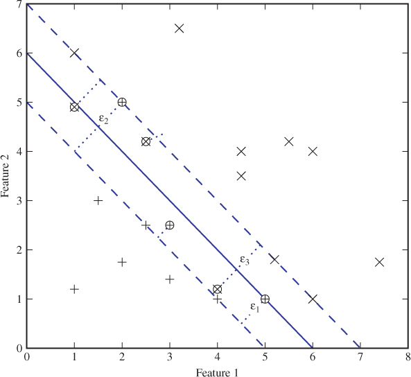
In SVM there are two quantities which determine the quality of the classification hyperplane. As in the linearly separable case, we still maintain two boundary hyperplanes at a distance M on either side of the classification hyperplane and parallel to it, and we want to maximise M. Obviously, some points will then be misclassified (cf. Figure 11.3), and for every training vector ![]() which falls on the wrong side of the relevant boundary plane, we define the error ϵi as the distance from
which falls on the wrong side of the relevant boundary plane, we define the error ϵi as the distance from ![]() to the boundary plane. Note that according to this definition, an error is not necessarily misclassified. Points which fall between the two boundary hyperplanes are considered errors, even if they still fall on the right side of the classifier hyperplane.
to the boundary plane. Note that according to this definition, an error is not necessarily misclassified. Points which fall between the two boundary hyperplanes are considered errors, even if they still fall on the right side of the classifier hyperplane.
Figure 11.3 Classification with errors
We build on the minimisation problem from the linearly separable case, where we only had to minimise ![]() . Now we also need to minimise the errors ϵi, which introduce slack in the constraints, that now become
. Now we also need to minimise the errors ϵi, which introduce slack in the constraints, that now become
![]()
The errors ϵi are also known as slack variables, because of their role in the constraints. For the sake of generality, we define ϵi = 0 for every training vector ![]() which falls on the right side of the boundary hyperplanes. Clearly ϵi ≥ 0 for all i. Training vectors which are correctly classified but fall between the boundaries will have
which falls on the right side of the boundary hyperplanes. Clearly ϵi ≥ 0 for all i. Training vectors which are correctly classified but fall between the boundaries will have ![]() , while misclassified vectors have ϵ ≥ 1.
, while misclassified vectors have ϵ ≥ 1.
Minimising ![]() and minimising the errors are conflicting objectives, and we need to find the right trade-off. In SVM, we simply add the errors to the cost function from the linearly separable case, multiplied by a constant scaling factor C to control the trade-off. Thus we get the following optimisation problem:
and minimising the errors are conflicting objectives, and we need to find the right trade-off. In SVM, we simply add the errors to the cost function from the linearly separable case, multiplied by a constant scaling factor C to control the trade-off. Thus we get the following optimisation problem:
A large C means that we prioritise minimising the errors and care less about the size of the margin. Smaller C will focus on maximising the margin at the expense of more errors.
The minimisation problem is solved in the same way as before, and we get the same definition of ![]() from (11.7):
from (11.7):
where the λi are found by solving the Wolfe dual, which can be simplified as
11.13 
11.14 
11.15 ![]()
It can be shown that, for all i, ϵi > 0 implies λi = C. Hence, training vectors which fall on the wrong side of the boundary hyperplane will make the heaviest contributions to the cost function.
11.2 The Kernel Function
The key to the success of SVM is the so-called kernel trick, which allows us to use the simple linear classifier discussed so far, and still solve non-linear classification problems. Both the linear SVM algorithm that we have discussed and the kernel trick are 1960s work, by Vapnik and Lerner (1963) and Aizerman et al. (1964), respectively. However, it was not until 1992 that Boser et al. (1992) combined the two. What is now considered to be the standard formulation of SVM is due to Cortes and Vapnik (1995), who introduced the soft margin. A comprehensive textbook presentation of the SVM algorithm is provided by Vapnik (2000).
The kernel trick applies to many classic classifiers besides SVM, so we will discuss some of the theory in general. First, let us illustrate the idea with an example.
11.2.1 Example: The XOR Function
A standard example of linearly non-separable problems is the XOR function. We have two features x1, x2 ∈ {0, 1} and two classes with labels given as y = x1 ⊕ x2 = x1 + x2 mod 2. This is illustrated in Figure 11.4(a). Clearly, no straight line can separate the two classes.
Figure 11.4 Feature space for the XOR problem: (a) in R2; (b) in R3
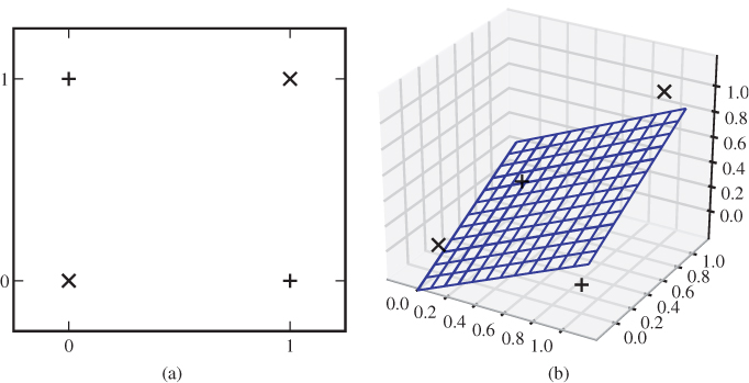
It is possible to separate the two classes by drawing a curve, but this would be a considerably more complex task, with more coefficients to optimise. Another alternative, which may not be intuitively obvious, is to add new features and transfer the problem into a higher-dimensional space where the classes become linearly separable.
In the XOR example, we could add a third feature x3 = x1x2. It is quite obvious that the four possible points (x1, x2, x3) are not in the same plane and hence they span ![]() . Consequently, a plane can be drawn to separate any two points from the other two. In particular, we can draw a plane to separate the pluses and the crosses, as shown in Figure 11.4(b).
. Consequently, a plane can be drawn to separate any two points from the other two. In particular, we can draw a plane to separate the pluses and the crosses, as shown in Figure 11.4(b).
11.2.2 The SVM Algorithm
The XOR example illustrates that some problems which are not linearly separable may become so by introducing additional features as functions of the existing ones. In the example, we introduced a mapping ![]() from a two-dimensional feature space to a three-dimensional one, by the rule that
from a two-dimensional feature space to a three-dimensional one, by the rule that
![]()
In general, we seek a mapping ![]() where m > n, so that the classification problem can be solved linearly in
where m > n, so that the classification problem can be solved linearly in ![]() .
.
Unfortunately, the higher dimension m may render the classification problem intractable. Not only would we have to deal with the computational cost of added unknowns, we would also suffer from the curse of dimensionality which we will discuss in Chapter 13. The typical result of excessively high dimension in machine learning is a model that does not generalise very well, i.e. we get poor accuracy in testing, even if the classes are almost separable in the training set.
The key to SVM is the observation that we can, in many cases, conceptually visualise the problem in ![]() but actually make all the calculations in
but actually make all the calculations in ![]() . First, remember that the feature vectors
. First, remember that the feature vectors ![]() in the linear classifier occur only in pairs, as part of the inner product
in the linear classifier occur only in pairs, as part of the inner product ![]() . To solve the problem in
. To solve the problem in ![]() , we thus need to be able to calculate
, we thus need to be able to calculate
11.16 ![]()
where · is the inner product in ![]() . That is all we ever need to know about
. That is all we ever need to know about ![]() or Φ.
or Φ.
This idea is known as the kernel trick, and K is called the kernel. A result known as Mercer's theorem states that if K satisfies certain properties, then there exists a Hilbert space H with a mapping ![]() with an inner product satisfying (11.16). The notion of a Hilbert space generalises Euclidean spaces, so
with an inner product satisfying (11.16). The notion of a Hilbert space generalises Euclidean spaces, so ![]() is just a special case of a Hilbert space, and any Hilbert space will do for the purpose of our classifier.
is just a special case of a Hilbert space, and any Hilbert space will do for the purpose of our classifier.
A kernel K, in this context, is any continuous function ![]() , where
, where ![]() is the feature space and
is the feature space and ![]() (symmetric). To apply Mercer's theorem, the kernel also has to be non-negative definite (Mercer's condition), that is
(symmetric). To apply Mercer's theorem, the kernel also has to be non-negative definite (Mercer's condition), that is
![]()
for all ![]() such that
such that
![]()
Note that we can use any kernel function satisfying Mercer's condition, without identifying the space H. The linear hyperplane defined by ![]() in H corresponds to a non-linear hypersurface in
in H corresponds to a non-linear hypersurface in ![]() defined by
defined by
![]()
Thus, the kernel trick gives us a convenient way to calculate a non-linear classifier while using the theory we have already developed for linear classifiers.
The kernel SVM classifier, for a given kernel K, is given simply by replacing all the dot products in the linear SVM solution by the kernel function. Hence we get
where the λi are found by solving
In the kernel SVM classifier, we can see that the number of support vectors may be critical to performance. When testing an object, by calculating ![]() , the kernel function has to be evaluated once for each support vector, something which may be costly. It can also be shown that the error rate may increase with increasing number of support vectors (Theodoridis and Koutroumbas, 2009).
, the kernel function has to be evaluated once for each support vector, something which may be costly. It can also be shown that the error rate may increase with increasing number of support vectors (Theodoridis and Koutroumbas, 2009).
There are four kernels commonly used in machine learning, as listed in Table 11.1. The linear kernel is just the dot product, and hence it is effectively as if we use no kernel at all. The result is a linear classifier in the original feature space. The polynomial kernel of degree d gives a classification hypersurface of degree d in the original feature space. The popular radial basis function that we used as the default in libSVM leads to a Hilbert space H of infinite dimension.
Table 11.1 Common kernel functions in machine learning
| linear | ||
| polynomial | γ ≥ 0 | |
| radial basis function | γ ≥ 0 | |
| sigmoid |
![]()
![]()
11.3 ν-SVM
There is a strong relationship between the SVM parameter C and the margin M. If C is large, a few outliers in the training set will have a serious impact on the classifier, because the error ϵi is considered expensive. If C is smaller, the classifier thinks little of such outliers and may achieve a larger margin. Even though the relationship between C and M is evident, it is not transparent. It is difficult to calculate the exact relationship and tune C analytically to obtain the desired result.
To get more intuitive control parameters, Schölkopf et al. (2000) introduced an alternative phrasing of the SVM problem, known as ν-SVM, which we present below. Note that ν-SVM works on exactly the same principles as the classic C-SVM already described. In particular, Chang and Lin (2000) showed that for the right choices of ν and C, both C-SVM and ν-SVM give the same solution.
In C-SVM, we normalised ![]() and w0 so that the boundary hyperplanes were defined as
and w0 so that the boundary hyperplanes were defined as
![]()
In ν-SVM, however, we leave the margin as a free variable ρ to be optimised, and let the boundary hyperplanes be given as
![]()
Thus, the minimisation problem can be cast as
11.17 ![]()
11.18 ![]()
11.19 ![]()
11.20 ![]()
The new parameter ν is used to weight the margin ρ in the cost function; the larger ν is, the more we favour a large margin at the expense of errors. Otherwise, the minimisation problem is similar to what we saw for C-SVM.
We will not go into all the details of solving the minimisation problem and analysing all the Lagrange multipliers. Interested readers can get a more complete discussion from Theodoridis and Koutroumbas (2009). Here we will just give some of the interesting conclusions. The Wolfe dual can be simplified to get
11.21 
11.22 
11.23 ![]()
11.24 
Contrary to the C-SVM problem, the cost function is now homogeneous quadratic. It can be shown that for every error ϵi > 0, we must have λi = 1/N. Furthermore, unless ρ = 0, we will get ∑λi = ν. Hence, the number of errors is bounded by νN, and the error rate on the training set is at most ν. In a similar fashion one can also show that the number of support vectors is at least νN.
The parameter ν thus gives a direct indication of the number of support vectors and the error rate on the training set. Finally, note that (11.23) and (11.24) imply ![]() . We also require ν ≥ 0, lest the margin be minimised.
. We also require ν ≥ 0, lest the margin be minimised.
11.4 Multi-class Methods
So far, we have viewed steganalysis as a binary classification problem, where we have exactly two possible class labels: ‘stego’ or ‘clean’. Classification problems can be defined for any number of classes, and in steganalysis this can be useful, for instance, to identify the stego-system used for embedding. A multi-class steganalyser could for instance aim to recognise class labels like ‘clean’, ‘F5’, ‘Outguess 0.2’, ‘JSteg’, ‘YASS’, etc.
The support-vector machine is an inherently binary classifier. It finds one hypersurface which splits the feature space in half, and it cannot directly be extended to the multi-class case. However, there are several methods which can be used to extend an arbitrary binary classifier to a multi-class classifier system.
The most popular method, known as one-against-all, will solve an M-class problem by employing M binary classifiers where each one considers one class against all others. Let C1, C2, … , CM denote the M classes. The ith constituent classifier is trained to distinguish between the two classes
![]()
and using the SVM notation it gives a classifier function ![]() . Let the labels be defined so that
. Let the labels be defined so that ![]() predicts
predicts ![]() and
and ![]() predicts
predicts ![]() .
.
To test an object ![]() , each classification function is evaluated at
, each classification function is evaluated at ![]() . If all give a correct classification, there will be one unique i so that
. If all give a correct classification, there will be one unique i so that ![]() , and we would conclude that
, and we would conclude that ![]() . To deal with the case where one or more binary classifiers may give an incorrect prediction, we note that a heuristic close to zero is more likely to be in error than one with a high absolute value. Thus the multi-class classifier rule will be to assume
. To deal with the case where one or more binary classifiers may give an incorrect prediction, we note that a heuristic close to zero is more likely to be in error than one with a high absolute value. Thus the multi-class classifier rule will be to assume
11.25 ![]()
An alternative approach to multi-class classification is one-against-one, which has been attributed to Knerr et al. (1990) (Hsu and Lin, 2002). This approach also splits the problem into multiple binary classification problems, but each binary class now compares one class Ci against one other Cj while ignoring all other classes. This requires ![]() binary classifiers, one for each possible pair of classes. This approach was employed in steganalysis by Pevný and Fridrich (2008). Several classifier rules exist for one-against-one classifier systems. The one used by Pevný and Fridrich is a simple majority voting rule. For each class Ci we count the binary classifiers that predict Ci, and we return the class Ci with the highest count. If multiple classes share the maximum count, we return one of them at random.
binary classifiers, one for each possible pair of classes. This approach was employed in steganalysis by Pevný and Fridrich (2008). Several classifier rules exist for one-against-one classifier systems. The one used by Pevný and Fridrich is a simple majority voting rule. For each class Ci we count the binary classifiers that predict Ci, and we return the class Ci with the highest count. If multiple classes share the maximum count, we return one of them at random.
A comparison of different multi-class systems based on the binary SVM classifier can be found in Hsu and Lin (2002). They conclude that the classification accuracy is similar for both one-against-one and one-against-all, but one-against-one is significantly faster to train. The libSVM package supports multi-class classification using one-against-one, simply because of the faster training process (Chang and Lin, 2011).
The faster training time in one-against-one is due to the size of the training set in the constituent classifiers. In one-against-all, the entire training set is required for every constituent decoder, while one-against-one only uses objects from two classes at a time. The time complexity of SVM training is roughly cubic in the number of training vectors, and the number of binary classifiers is only quadratic in M. Hence, the one-against-one will be significantly faster for large M.
An additional benefit of one-against-one is flexibility and extendability. If a new class has to be introduced with an existing trained classifier, one-against-all requires complete retraining of all the constituent classifiers, because each requires the complete training set which is extended with a new class. This is not necessary in one-against-one. Since each classifier only uses two classes, all the existing classifiers are retained unmodified. We simply need to add M new constituent classifiers, pairing the new class once with each of the old ones.
11.5 One-class Methods
The two- and multi-class methods which we have discussed so far all have to be trained with actual steganograms as well as clean images. Hence they will never give truly blind classifiers, but be tuned to whichever stego-systems we have available when we create the training set. Even though unknown algorithms may sometimes cause artifacts similar to known algorithms, and thus be detectable, this is not the case in general. The ideal blind steganalyser should be able to detect steganograms from arbitrary, unknown stego-systems, even ones which were previously unknown to the steganalyst. In this case, there is only one class which is known at the time of training, namely the clean images. Since we do not know all stego-systems, we cannot describe the complement of this class of clean images.
One-class classification methods provide a solution. They are designed to be trained on only a single class, such as clean images. They distinguish between normal objects which look like training images, and abnormal objects which do not fit the model. In the case of steganalysis, abnormal objects are assumed to be steganograms. This leads to truly blind steganalysis; no knowledge about the steganographic embedding is used, neither in algorithm design nor in the training phase. Thus, at least in principle, we would expect a classifier which can detect arbitrary and unknown steganalytic systems.
There is a one-class variant of SVM based on ν-SVM, described by Schölkopf et al. (2001). Instead of aiming to fit a hyperplane between the two known classes in the training set, it attempts to fit a tight hypersphere around the whole training set. In classification, objects falling within the hypersphere are assumed to be normal or negative, and those outside are considered abnormal or positive.
11.5.1 The One-class SVM Solution
A hypersphere with radius R centred at a point ![]() is defined by the equation
is defined by the equation
![]()
To train the one-class SVM, we thus need to find the optimal ![]() and optimal R for the classification hypersphere.
and optimal R for the classification hypersphere.
Just as in the two-class case, we will want to accept a number of errors, that is training vectors which fall at a distance ϵi outside the hypersphere. This may not be quite as obvious as it was in the non-separable case, where errors would exist regardless of the solution. In the one-class case there is no second class to separate from at the training stage, and choosing R large enough, everything fits within the hypersphere. In contrast, the second class will appear in testing, and we have no reason to expect the two classes to be separable. Accepting errors in training means that the odd outliers will not force an overly large radius that would give a high false negative rate.
The minimisation problem is similar to the one we have seen before. Instead of maximising the margin, we now aim to keep the hypersphere as small as possible to give a tight description of the training set and limit false negatives as much as possible. Thus R2 takes the place of ![]() in the minimisation problem. As before we also need to minimise the errors ϵi. This gives the following minimisation problem:
in the minimisation problem. As before we also need to minimise the errors ϵi. This gives the following minimisation problem:
where Φ is the mapping into the higher-dimensional space induced by the chosen kernel K, and ![]() is the centre of the hypersphere in the higher-dimensional space. Again, we will skip the details of the derivation, and simply state the major steps and conclusions. The dual problem can be written as
is the centre of the hypersphere in the higher-dimensional space. Again, we will skip the details of the derivation, and simply state the major steps and conclusions. The dual problem can be written as
and the solution, defined as the centre of the hypersphere, is
![]()
The squared distance between a point ![]() and the hypersphere centre
and the hypersphere centre ![]() is given by
is given by
![]()
A point is classified as a positive if this distance is greater than R2 and a negative if it is smaller. Hence we write the classification function as
![]()
11.5.2 Practical Problems
The one-class SVM introduces a new, practical problem compared to the two-class case. The performance depends heavily on the SVM parameter ν or C and on the kernel parameters γ. In the two-class case, we solved this problem using a grid search with cross-validation. In the multi-class case, we can perform separate grid searches to tune each of the constituent (binary) classifiers. With a one-class training set, there is no way to carry out a cross-validation of accuracy.
The problem is that cross-validation estimates the accuracy, and the grid search seeks the maximum accuracy. With only one class we can only check for false positives; there is no sample of true positives which could be used to check for false negatives. Hence the grid search would select the largest R in the search space, and it would say nothing about the detection rate when we start testing on the second class.
Any practical application has to deal with the problem of parameter tuning. If we want to keep the true one-class training phase, there may actually be no way to optimise C or ν, simply because we have no information about the overlap between the training class and other classes. One possibility is to use a system of two-stage training. This requires a one-class training set T1 which is used to train the support vector machine for given parameters C or ν. Then, we need a multi-class training set T2 which can be used in lieu of cross-validation to test the classifier for each parameter choice. This allows us to make a grid search similar to the one in the binary case. Observe that we called T2 a training set, and not a test set. The parameters ν or C will depend on T2 and hence the tests done on T2 are not independent and do not give information about the performance on unknown data. Where T1 is used to train the system with respect to the SVM hypersphere, T2 is used to train it with respect to C or ν.
Similar issues may exist with respect to the kernel parameters, such as γ in the RBF. Since the parameter changes the kernel and thus the higher-dimensional space used, we cannot immediately assume that the radius which we aim to minimise is comparable for varying γ. Obviously, we can use the grid search with testing on T2 to optimise γ together with C or ν.
11.5.3 Multiple Hyperspheres
There are only few, but all the more interesting examples of one-class classifiers for steganalysis in the literature. Lyu and Farid (2004) used one-class SVM with Farid-72, but demonstrated that the hypersphere was the wrong shape to cover the training set. Using the one-class SVM system as described, they had accuracies around 10–20%.
Lyu and Farid suggested instead to use multiple, possibly overlapping hyperspheres to describe the training set. By using more than one hypersphere, each hypersphere would become more compact, with a smaller radius. Many hyperspheres together can cover complex shapes approximately. With six hyperspheres they achieved accuracies up to 70%.
Clearly, the SVM framework in itself does not support a multi-hypersphere model. However, if we can partition the training set into a sensible number of subsets, or clusters, we can make a one-class SVM model for each such cluster. Such a partition can be created using a clustering algorithm, like the ones we will discover in Section 12.4. Lyu and Farid (2004) used k-means clustering.
In experiments, the one-class SVM classifier with multiple hyperspheres tended to outperform two-class classifiers for short messages, while two-class classifiers were better for longer messages. The false positive rate was particularly low for the one-class classifiers. It should be noted, however, that this approach has not been extensively tested in the literature, and the available data are insufficient to conclude.
11.6 Summary
Support vector machines have proved to give a flexible framework, and off-the-shelf software packages provide one-, two- and multi-class classification. The vast majority of steganalysis research has focused on two-class classifiers. There is not yet sufficient data available to say much about the performance and applicability of one- and multi-class methods in general, and this leaves an interesting open problem.