
Chapter 13
Feature Selection and Evaluation
Selecting the right features for classification is a major task in all areas of pattern matching and machine learning. This is a very difficult problem. In practice, adding a new feature to an existing feature vector may increase or decrease performance depending on the features already present. The search for the perfect vector is an NP-complete problem. In this chapter, we will discuss some common techniques that can be adopted with relative ease.
13.1 Overfitting and Underfitting
In order to get optimal classification accuracy, the model must have just the right level of complexity. Model complexity is determined by many factors, one of which is the dimensionality of the feature space. The more features we use, the more degrees of freedom we have to fit the model, and the more complex it becomes.
To understand what happens when a model is too complex or too simple, it is useful to study both the training error rate ![]() and the testing error rate
and the testing error rate ![]() . We are familiar with the testing error rate from Chapter 10, where we defined the accuracy as
. We are familiar with the testing error rate from Chapter 10, where we defined the accuracy as ![]() , while the training error rate
, while the training error rate ![]() is obtained by testing the classifier on the training set. Obviously, it is only the testing error rate which gives us any information about the performance on unknown data.
is obtained by testing the classifier on the training set. Obviously, it is only the testing error rate which gives us any information about the performance on unknown data.
If we start with a simple model with few features and then extend it by adding new features, we will typically see that ![]() decreases. The more features, the better we can fit the model to the training data, and given enough features and thus degrees of freedom, we can fit it perfectly to get
decreases. The more features, the better we can fit the model to the training data, and given enough features and thus degrees of freedom, we can fit it perfectly to get ![]() . This is illustrated in Figure 13.1, where we see the monotonically decreasing training error rate.
. This is illustrated in Figure 13.1, where we see the monotonically decreasing training error rate.
Figure 13.1 Training error rate and testing error rate for varying dimensionality (for illustration)
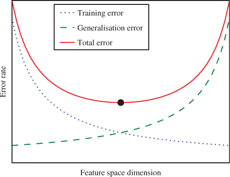
Now consider ![]() in the same way. In the beginning we would tend to have
in the same way. In the beginning we would tend to have ![]() , where both decrease with increasing complexity. This situation is known as underfitting. The model is too simple to fit the data very well, and therefore we get poor classification on the training and test set alike. After a certain point,
, where both decrease with increasing complexity. This situation is known as underfitting. The model is too simple to fit the data very well, and therefore we get poor classification on the training and test set alike. After a certain point, ![]() will tend to rise while
will tend to rise while ![]() continues to decline. It is natural that
continues to decline. It is natural that ![]() declines as long as degrees of freedom are added. When
declines as long as degrees of freedom are added. When ![]() starts to increase, so that
starts to increase, so that ![]() , it means that the model no longer generalises for unknown data. This situation is known as overfitting, where the model has become too complex. Overfitting can be seen as support for Occam's Razor, the principle that, other things being equal, the simpler theory is to be preferred over the more complex one. An overfitted solution is inferior because of its complexity.
, it means that the model no longer generalises for unknown data. This situation is known as overfitting, where the model has become too complex. Overfitting can be seen as support for Occam's Razor, the principle that, other things being equal, the simpler theory is to be preferred over the more complex one. An overfitted solution is inferior because of its complexity.
It may be counter-intuitive that additional features can sometimes give a decrease in performance. After all, more features means more information, and thus, in theory, the classifier should be able to make a better decision. This phenomenon is known as the curse of dimensionality. High-dimensionality feature vectors mean that the classifier gets many degrees of freedom and the model can be fitted perfectly to the training data. Thus, the model will not only capture statistical properties of the different classes, but also random noise elements which are peculiar for each individual object. Such a model generalises very poorly for unseen objects, leading to the discrepancy ![]() . Another way to view the curse of dimensionality is to observe that the distance between points in space increases as the dimension of the space increases. Thus the observations we make become more scattered and it seems reasonable that less can be learnt from them.
. Another way to view the curse of dimensionality is to observe that the distance between points in space increases as the dimension of the space increases. Thus the observations we make become more scattered and it seems reasonable that less can be learnt from them.
There are other causes of overfitting, besides the curse of dimensionality. In the case of SVM, for instance, tuning the parameter ![]() (or
(or ![]() ) is critical, as it controls the weighting of the two goals of minimising the (training) errors and maximising the margin. If
) is critical, as it controls the weighting of the two goals of minimising the (training) errors and maximising the margin. If ![]() is too large, the algorithm will prefer a very narrow margin to avoid errors, and a few outliers which are atypical for the distribution can have an undue impact on the classifier. This would push
is too large, the algorithm will prefer a very narrow margin to avoid errors, and a few outliers which are atypical for the distribution can have an undue impact on the classifier. This would push ![]() up and
up and ![]() down, indicating another example of overfitting. Contrarily, if
down, indicating another example of overfitting. Contrarily, if ![]() is too small, the importance of errors is discounted, and the classifier will accept a fairly high
is too small, the importance of errors is discounted, and the classifier will accept a fairly high ![]() giving evidence of underfitting. Thus, the problems with under- and overfitting make up one of the motivations behind the grid search and cross-validation that we introduced in Section 3.3.2.
giving evidence of underfitting. Thus, the problems with under- and overfitting make up one of the motivations behind the grid search and cross-validation that we introduced in Section 3.3.2.
13.1.1 Feature Selection and Feature Extraction
In order to avoid the curse of dimensionality, it is often necessary to reduce the dimension of the feature space. There are essentially two approaches to this, namely feature selection and feature extraction.
Feature extraction is the most general approach, aiming to map feature vectors in ![]() into some smaller space
into some smaller space ![]() (
(![]() ). Very often, almost all of the sample feature vectors are approximately contained in some
). Very often, almost all of the sample feature vectors are approximately contained in some ![]() -dimensional subspace of
-dimensional subspace of ![]() . If this is the case, we can project all the feature vectors into
. If this is the case, we can project all the feature vectors into ![]() without losing any structure, except for the odd outlier. Even though the mapping
without losing any structure, except for the odd outlier. Even though the mapping ![]() may in general sacrifice information, when the sample feature vectors really span a space of dimension greater than
may in general sacrifice information, when the sample feature vectors really span a space of dimension greater than ![]() , the resulting feature vectors in
, the resulting feature vectors in ![]() may still give superior classification by avoiding overfitting. There are many available techniques for feature extraction, with principal component analysis (PCA) being one of the most common examples. In steganalysis, Xuan et al. (2005b) used a feature extraction method of Guorong et al. (1996), based on the Bhattacharyya distance. The details are beyond the scope of this book, and we will focus on feature selection in the sequel.
may still give superior classification by avoiding overfitting. There are many available techniques for feature extraction, with principal component analysis (PCA) being one of the most common examples. In steganalysis, Xuan et al. (2005b) used a feature extraction method of Guorong et al. (1996), based on the Bhattacharyya distance. The details are beyond the scope of this book, and we will focus on feature selection in the sequel.
Feature selection is a special and limited case of feature extraction. Writing a feature vector as ![]() , we are only considering maps
, we are only considering maps ![]() which can be written as
which can be written as
![]()
for some subset ![]() . In other words, we select individual features from the feature vector
. In other words, we select individual features from the feature vector ![]() , ignoring the others completely.
, ignoring the others completely.
In addition to reducing the dimensionality to avoid overfitting, feature selection is also a good help to interpret the problem. A classifier taking a 1000-D feature vector to get a negligible error rate may be great to solve the steganalyser's practical problem. However, it is almost impossible to analyse, and although the machine can learn a lot, the user learns rather little.
If we can identify a low-dimensional feature vector with decent classification performance, we can study each feature and find out how and why it is affected by the embedding. Thus a manageable number of critical artifacts can be identified, and the design of new steganographic systems can focus on eliminating these artifacts. Using feature selection in this context, we may very well look for a feature vector giving inferior classification accuracy. The goal is to find one which is small enough to be manageable and yet explains most of the detectability. Because each feature is either used or ignored, feature selection gives easy-to-use information about the artifacts detected by the classifier.
13.2 Scalar Feature Selection
Scalar feature selection aims to evaluate individual, scalar features independently. Although such an approach disregards dependencies between the different features in a feature vector, it still has its uses. An important benefit is that the process scales linearly in the number of candidate features. There are many heuristics and approaches which can be used. We will only have room for ANOVA, which was used to design one of the pioneering feature vectors in steganalysis.
13.2.1 Analysis of Variance
Analysis of variance (ANOVA) is a technique for hypothesis testing, aiming to determine if a series of sub-populations have the same mean. In other words, if a population is made up of a number of disjoint classes ![]() and we observe a statistic
and we observe a statistic ![]() , we want to test the null hypothesis:
, we want to test the null hypothesis:
![]()
where ![]() is the mean of
is the mean of ![]() when drawn from
when drawn from ![]() . A basic requirement for any feature in machine learning is that it differs between the different classes
. A basic requirement for any feature in machine learning is that it differs between the different classes ![]() . Comparing the means of each class is a reasonable criterion.
. Comparing the means of each class is a reasonable criterion.
Avciba![]() et al. (2003) started with a large set of features which they had studied in a different context and tested them on a steganalytic problem. They selected the ten features with the lowest
et al. (2003) started with a large set of features which they had studied in a different context and tested them on a steganalytic problem. They selected the ten features with the lowest ![]() -value in the hypothesis test to form their IQM feature vector (see Section 6.2). It is true that a feature may be discarded because it has the same mean for all classes and still have some discriminatory power. However, the ANOVA test does guarantee that those features which are selected will have discriminatory power.
-value in the hypothesis test to form their IQM feature vector (see Section 6.2). It is true that a feature may be discarded because it has the same mean for all classes and still have some discriminatory power. However, the ANOVA test does guarantee that those features which are selected will have discriminatory power.
There are many different ANOVA designs, and entire books are devoted to the topic. We will give a short presentation of one ANOVA test, following Johnson and Wichern (1988), but using the terminology of steganalysis and classification. We have a feature ![]() representing some property of an object
representing some property of an object ![]() which is drawn randomly from a population consisting of a number of disjoint classes
which is drawn randomly from a population consisting of a number of disjoint classes ![]() , for
, for ![]() . Thus
. Thus ![]() is a stochastic variable. We have a number of observations
is a stochastic variable. We have a number of observations ![]() , where
, where ![]() and
and ![]() is drawn from
is drawn from ![]() .
.
There are three assumptions underlying ANOVA:
The first assumption should be no surprise. We depend on this whenever we test a classifier to estimate error probabilities too, and it amounts to selecting media objects randomly and independently. The third assumption, on the distribution, can be relaxed if the sample is sufficiently large, due to the Central Limit Theorem.
The second assumption, that the variances are equal, gives cause for concern. A priori, there is no reason to think that steganographic embedding should not have an effect on the variance instead of or in addition to the mean. Hence, one will need to validate this assumption if the quantitative conclusions made from the ANOVA test are important.
To understand the procedure, it is useful to decompose the statistic or feature into different effects. Each observation can be written as a sum
![]()
where ![]() is the mean which is common for the entire population and
is the mean which is common for the entire population and ![]() is a so-called class effect which is the difference between the class mean and the population mean, i.e.
is a so-called class effect which is the difference between the class mean and the population mean, i.e. ![]() . The last term can be called a random error
. The last term can be called a random error ![]() , that is the effect due to the individuality of each observation.
, that is the effect due to the individuality of each observation.
With the notation of the decomposition, the null hypothesis may be rephrased as
![]()
In practice the means are unknown, but we can make an analogous decomposition using sample means as follows:
13.1 ![]()
for ![]() and
and ![]() . This can be written as a vector equation,
. This can be written as a vector equation,
13.2 ![]()
where ![]() is an all-one vector, and
is an all-one vector, and
We are interested in a decomposition of the sample variance ![]() , where squaring denotes an inner product of a vector and itself. We will show that
, where squaring denotes an inner product of a vector and itself. We will show that
13.3 ![]()
This equation follows from the fact that the three vectors on the right-hand side of (13.2) are orthogonal. In other words, ![]() ,
, ![]() and
and ![]() regardless of the actual observations. To demonstrate this, we will give a detailed derivation of (13.3).
regardless of the actual observations. To demonstrate this, we will give a detailed derivation of (13.3).
Subtracting ![]() on both sides of (13.1) and squaring gives
on both sides of (13.1) and squaring gives
![]()
and summing over ![]() , while noting that
, while noting that ![]() , gives
, gives
Next, summing over ![]() , we get
, we get
which is equivalent to (13.3).
The first term, ![]() , is the component of variance which is explained by the class. The other component,
, is the component of variance which is explained by the class. The other component, ![]() , is unexplained variance. If
, is unexplained variance. If ![]() is true, the unexplained variance
is true, the unexplained variance ![]() should be large compared to the explained variance
should be large compared to the explained variance ![]() . A standard
. A standard ![]() -test can be used to compare the two.
-test can be used to compare the two.
It can be shown that ![]() has
has ![]() degrees of freedom, while
degrees of freedom, while ![]() has
has ![]() degrees of freedom, where
degrees of freedom, where ![]() . Thus the
. Thus the ![]() statistic is given as
statistic is given as
![]()
which is ![]() distributed with
distributed with ![]() and
and ![]() degrees of freedom. The
degrees of freedom. The ![]() -value is the probability that a random
-value is the probability that a random ![]() -distributed variable is greater than or equal to the observed value
-distributed variable is greater than or equal to the observed value ![]() as defined above. This probability can be found in a table or by using statistics software. We get the same ordering whether we rank features by
as defined above. This probability can be found in a table or by using statistics software. We get the same ordering whether we rank features by ![]() -value or by
-value or by ![]() -value.
-value.
13.3 Feature Subset Selection
Given a set of possible features ![]() , feature selection aims to identify a subset
, feature selection aims to identify a subset ![]() which gives the best possible classification. The features in the optimal subset
which gives the best possible classification. The features in the optimal subset ![]() do not have to be optimal individually. An extreme and well-known example can be seen in the XOR example from Section 11.2.1. We have two features
do not have to be optimal individually. An extreme and well-known example can be seen in the XOR example from Section 11.2.1. We have two features ![]() and
and ![]() and a class label
and a class label ![]() . Let
. Let ![]() with a 50/50 probability distribution, and both
with a 50/50 probability distribution, and both ![]() and
and ![]() are independent of
are independent of ![]() , that is
, that is
![]()
Thus, neither feature ![]() is individually useful for predicting
is individually useful for predicting ![]() . Collectively, in contrast, the joint variable
. Collectively, in contrast, the joint variable ![]() gives complete information about
gives complete information about ![]() , giving a perfect classifier.
, giving a perfect classifier.
In practice, we do not expect such an extreme situation, but it is indeed very common that the usefulness of some features depends heavily on other features included. Two types of dependence are possible. In the XOR example, we see that features reinforce each other. The usefulness of a group of features is more than the sum of its components. Another common situation is where features are redundant, in the sense that the features are highly correlated and contain the same information about the class label. Then the usefulness of the group will be less than the sum of its components.
It is very hard to quantify the usefulness of features and feature vectors, and thus examples necessarily become vague. However, we can note that Cartesian calibration as discussed in Chapter 9 aims to construct features which reinforce each other. The calibrated features are often designed to have the same value for a steganogram and the corresponding cover image, and will then have no discriminatory power at all. Such features are invented only to reinforce the corresponding uncalibrated features. We also have reason to expect many of the features in the well-known feature vectors to be largely redundant. For instance, when we consider large feature vectors where all the features are calculated in a similar way, like SPAM or Shi et al.'s Markov features, it is reasonable to expect the individual features to be highly correlated. However, it is not easy to identify which or how many can safely be removed.
Subset selection consists of two sub-problems. Firstly, we need a method to evaluate the usefulness of a given candidate subset, and we will refer to this as subset evaluation. Secondly, we need a method for subset search to traverse possible subsets looking for the best one we can find. We will consider the two sub-problems in turn.
13.3.1 Subset Evaluation
The most obvious way to evaluate a subset of features is to train and test a classifier and use a performance measure such as the accuracy, as the heuristic of the feature subset. This gives rise to so-called wrapper search; the feature selection algorithm wraps around the classifier. This approach has the advantage of ranking feature vectors based exactly on how they would perform with the chosen classifier. The down-side is that the training/testing cycle can be quite expensive.
The alternative is so-called filter search, where we use some evaluation heuristic independent of the classifier. Normally, such heuristics will be faster than training and testing a classifier, but it may also be an advantage to have a ranking criterion which is independent of the classifier to be used.
The main drawback of wrapper search is that it is slow to train. This is definitely the case for state-of-the-art classifiers like SVM, but there are many classifiers which are faster to train at the expense of accuracy. Such fast classifiers can be used to design a filter search. Thus we would use the evaluation criterion of a wrapper search, but since the intention is to use the selected features with arbitrary classifiers, it is properly described as a filter search. Miche et al. (2006) propose a methodology for feature selection in steganalysis, where they use a ![]() nearest neighbours (K-NN) classifier for the filter criterion and SVM for the classification.
nearest neighbours (K-NN) classifier for the filter criterion and SVM for the classification.
The ![]() nearest neighbour algorithm takes no time at all to train; all the calculations are deferred until classification. The entire training set is stored, with a set of feature vectors
nearest neighbour algorithm takes no time at all to train; all the calculations are deferred until classification. The entire training set is stored, with a set of feature vectors ![]() and corresponding labels
and corresponding labels ![]() . To predict the class of a new feature vector
. To predict the class of a new feature vector ![]() , the Euclidean distance
, the Euclidean distance ![]() is calculated for each
is calculated for each ![]() , and the
, and the ![]() nearest neighbours
nearest neighbours ![]() are identified. The predicted label is taken as the most frequent class label among the
are identified. The predicted label is taken as the most frequent class label among the ![]() nearest neighbours
nearest neighbours ![]() .
.
Clearly, the classification time with ![]() nearest neighbour depends heavily on the size of the training set. The distance calculation is
nearest neighbour depends heavily on the size of the training set. The distance calculation is ![]() , where
, where ![]() is the number of features and
is the number of features and ![]() is the number of training vectors. SVM, in contrast, may be slow to train, but the classification time is independent of
is the number of training vectors. SVM, in contrast, may be slow to train, but the classification time is independent of ![]() . Thus
. Thus ![]() nearest neighbour is only a good option if the training set can be kept small. We will present a couple of alternative filter criteria later in this chapter, and interested readers can find many more in the literature.
nearest neighbour is only a good option if the training set can be kept small. We will present a couple of alternative filter criteria later in this chapter, and interested readers can find many more in the literature.
13.3.2 Search Algorithms
Subset search is a general algorithmic problem which appears in many different contexts. Seeking a subset ![]() maximising some heuristic
maximising some heuristic ![]() , there are
, there are ![]() potential solutions. It is clear that we cannot search them all except in very small cases. Many different algorithms have been designed to search only a subset of the possible solutions in such a way that a near-optimal solution can be expected.
potential solutions. It is clear that we cannot search them all except in very small cases. Many different algorithms have been designed to search only a subset of the possible solutions in such a way that a near-optimal solution can be expected.
In sequential forward selection, we build our feature set ![]() , starting with an empty set and adding one feature per round. Considering round
, starting with an empty set and adding one feature per round. Considering round ![]() , let
, let ![]() be the features already selected. For each candidate feature
be the features already selected. For each candidate feature ![]() , we calculate our heuristic for
, we calculate our heuristic for ![]() . The
. The ![]() th feature
th feature ![]() is chosen as the one maximising the heuristic.
is chosen as the one maximising the heuristic.
Where forward selection starts with an empty set which is grown to the desired size, backward selection starts with a large set of features which is pruned by removing one feature every round. Let ![]() be the set of all features under consideration in round
be the set of all features under consideration in round ![]() . To form the feature set for round
. To form the feature set for round ![]() , we find
, we find ![]() by solving
by solving
![]()
and set ![]() .
.
Sequential methods suffer from the fact that once a given feature has been accepted (in forward search) or rejected (in backward search), this decision is final. There is no way to correct a bad choice later. A straight forward solution to this problem is to alternate between forward and backward search, for instance the classic ‘plus ![]() , take away
, take away ![]() ’ search, where we alternately make
’ search, where we alternately make ![]() steps forward and then
steps forward and then ![]() steps backward. If we start with an empty set, we need
steps backward. If we start with an empty set, we need ![]() . The backward steps can cancel bad choices in previous forward steps and vice versa.
. The backward steps can cancel bad choices in previous forward steps and vice versa.
The simple ‘plus ![]() , take away
, take away ![]() ’ algorithm can be made more flexible by making
’ algorithm can be made more flexible by making ![]() and
and ![]() dynamic and data dependent. In the classic floating search of Pudil et al. (1994), a backward step should only be performed if it leads to an improvement. It works as follows:
dynamic and data dependent. In the classic floating search of Pudil et al. (1994), a backward step should only be performed if it leads to an improvement. It works as follows:
The search continues until the heuristic converges.
13.4 Selection Using Information Theory
One of the 20th-century milestones in engineering was Claude Shannon's invention of a quantitative measure of information (Shannon, 1948). This led to an entirely new field of research, namely information theory. The original application was in communications, but it has come to be used in a range of other areas as well, including machine learning.
13.4.1 Entropy
Consider two stochastic variables ![]() and
and ![]() . Information theory asks, how much information does
. Information theory asks, how much information does ![]() contain about
contain about ![]() ? In communications,
? In communications, ![]() may be a transmitted message and
may be a transmitted message and ![]() is a received message, distorted by noise. In machine learning, it is interesting to ask how much information a feature or feature vector
is a received message, distorted by noise. In machine learning, it is interesting to ask how much information a feature or feature vector ![]() contains about the class label
contains about the class label ![]() .
.
Let's first define the uncertainty or entropy ![]() of a discrete stochastic variable
of a discrete stochastic variable ![]() , as follows:
, as follows:
![]()
Note that the base of the logarithm matters little. Changing the base would only scale the expression by a constant factor. Using base 2, we measure the entropy in bits. With the natural logarithm, we measure it in nats.
Shannon's definition is clearly inspired by the concept of entropy from thermodynamics, but the justification is based on a number of intuitive axioms about uncertainty, or ‘lack of information’. Shannon (1948) motivated the definition with three key properties or axioms:
- The entropy is continuous in
 for each
  .
. - If the distribution is uniform, then
 is a monotonically increasing function in
  .
. - ‘If a choice be broken down into two successive choices, the original
 should be the weighted sum of the individual values of
  .’
.’
The last of these properties may be a little harder to understand than the first two. In order to ‘break down’ the entropy into successive choices, we need to extend the concept of entropy for joint and conditional distributions. Joint entropy is straightforward. Given two random variables ![]() and
and ![]() , we can consider the joint random variable
, we can consider the joint random variable ![]() . Using the joint probability distribution, the joint entropy is given as
. Using the joint probability distribution, the joint entropy is given as
If the two variables ![]() and
and ![]() are independent, it is trivial to break down the
are independent, it is trivial to break down the ![]() into successive choices:
into successive choices:
13.4 
giving us a sum of individual entropies as required by the axiom.
In the example above, the remaining entropy after observing ![]() is given as
is given as ![]() , but this is only because
, but this is only because ![]() and
and ![]() are independent. Regardless of what we find from observing
are independent. Regardless of what we find from observing ![]() , the entropy of
, the entropy of ![]() is unchanged. In general, however, the entropy of
is unchanged. In general, however, the entropy of ![]() will change, and vary depending on what
will change, and vary depending on what ![]() is. This is determined by the conditional probability distribution
is. This is determined by the conditional probability distribution ![]() . Every possible value of
. Every possible value of ![]() gives a different distribution for
gives a different distribution for ![]() , each with an entropy given as
, each with an entropy given as
![]()
where we can see the weighted sum of constituent entropies for different observations of the first variable ![]() . We define the conditional entropy
. We define the conditional entropy ![]() as the expected value of
as the expected value of ![]() when
when ![]() is drawn at random from the corresponding probability distribution. In other words,
is drawn at random from the corresponding probability distribution. In other words,
It is straightforward, following the lines of (13.4), to see that
![]()
as a Bayes law for entropy. This shows how a choice in general can be broken down into successive choices. The total entropy is given as the unconditional entropy of the first choice and the conditional entropy of the second choice. Moreover, the conditional entropy is the weighted sum (average) of the possible entropies corresponding to different outcomes of the first choice, as Shannon stipulated.
We can also see that a deterministic variable, that is one with a single possible outcome ![]() with
with ![]() , has zero entropy as there is no uncertainty in this case. Given a fixed size
, has zero entropy as there is no uncertainty in this case. Given a fixed size ![]() we see that
we see that ![]() is maximised for the uniform distribution. This is logical because then everything is equally likely, and any attempt at prediction would be pure guesswork, or in other words, maximum uncertainty.
is maximised for the uniform distribution. This is logical because then everything is equally likely, and any attempt at prediction would be pure guesswork, or in other words, maximum uncertainty.
13.4.2 Mutual Information
When the entropy of one variable ![]() changes, from our viewpoint, as a result of observing a different variable
changes, from our viewpoint, as a result of observing a different variable ![]() , it is reasonable to say that
, it is reasonable to say that ![]() gives us information about
gives us information about ![]() . Entropy gives us the means to quantify this information.
. Entropy gives us the means to quantify this information.
The information ![]() gives about
gives about ![]() can be defined as the change in the entropy of
can be defined as the change in the entropy of ![]() as a result of observing
as a result of observing ![]() , or formally
, or formally
13.5 ![]()
The quantity ![]() is called the mutual information between
is called the mutual information between ![]() and
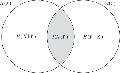
and ![]() , and it is indeed mutual, or symmetric, because
, and it is indeed mutual, or symmetric, because
This equation is commonly illustrated with the Venn diagram in Figure 13.2. We can also rewrite the definition of ![]() purely in terms of probabilities, as follows:
purely in terms of probabilities, as follows:
13.6 
Figure 13.2 Venn diagram showing the various entropies and mutual information of two random variables ![]() and
and ![]()
We will also need the conditional mutual information. The definition of ![]()
![]() follows directly from the above, replacing the conditional probability distributions of
follows directly from the above, replacing the conditional probability distributions of ![]() and
and ![]() given
given ![]() . The conditional mutual information is given as the weighted average, in the same way as we defined conditional entropy:
. The conditional mutual information is given as the weighted average, in the same way as we defined conditional entropy:
![]()
The entropy and mutual information are defined from the probability distribution, which is a theoretical and unobservable concept. In practice, we will have to estimate the quantities. In the discrete case, this is straightforward and uncontroversial. We simply use relative frequencies to estimate probabilities, and calculate the entropy and mutual information substituting estimates for the probabilities.
![]()
![]()
![]()
There is a strong relationship between mutual information and entropy on the one hand, and classifier performance on the other.
Note that the entropy ![]() is the regular, discrete entropy of
is the regular, discrete entropy of ![]() . It is only the conditional variable
. It is only the conditional variable ![]() which is continuous, but
which is continuous, but ![]() is still well-defined as the expected value of
is still well-defined as the expected value of ![]() .
.
![]()
![]()
![]()
![]()
13.4.3 Multivariate Information
To present the general framework for feature selection using information theory, we will need multivariate mutual information. This can be defined in many different ways. Yeung (2002) develops information theory in terms of measure theory, where entropy, mutual information and multivariate information are special cases of the same measure. As beautiful as this framework is, there is no room for the mathematical detail in this book. We give just the definition of multivariate information, as follows.
![]()
We can clearly see traces of the inclusion/exclusion theorem applied to some measure ![]() . It is easily checked that mutual information is a special case where
. It is easily checked that mutual information is a special case where ![]() by noting that
by noting that
![]()
We note that the definition also applies to singleton and empty sets, where ![]() and
and ![]() . The first author to generalise mutual information for three or more variables was McGill (1954), who called it interaction information. His definition is quoted below, but it can be shown that interaction information and multivariate mutual information are equivalent (Yeung, 2002). We will use both definitions in the sequel.
. The first author to generalise mutual information for three or more variables was McGill (1954), who called it interaction information. His definition is quoted below, but it can be shown that interaction information and multivariate mutual information are equivalent (Yeung, 2002). We will use both definitions in the sequel.
![]()
Note that ![]() is not in any way considered as a joint stochastic variable
is not in any way considered as a joint stochastic variable ![]() . Considering a single joint variable
. Considering a single joint variable ![]() gives the interaction information
gives the interaction information
![]()
which is the joint entropy, while ![]() leads to
leads to
![]()
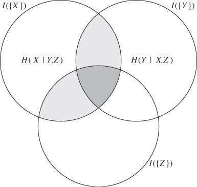
which is the mutual information. Considering three variables, the interaction information is given as
![]()
which does not coincide with the mutual information ![]() , nor with
, nor with ![]() . The relationship is visualised in Figure 13.3.
. The relationship is visualised in Figure 13.3.
Figure 13.3 Venn diagram showing interaction information for three random variables. The dark grey area is the third-order interaction information ![]() . The total grey area (dark and light) is the mutual information
. The total grey area (dark and light) is the mutual information ![]()
![]()
Our interest in the multivariate mutual information comes from the fact that we can use it to estimate the pairwise mutual information of joint stochastic variables. The following theorem is taken from Brown (2009).
![]()
We omit the proof, which is straightforward but tedious. An interested reader can find it by inserting for the definition of interaction information in each term on the right-hand side.
Clearly, ![]() is a suitable heuristic for feature selection. A good feature set
is a suitable heuristic for feature selection. A good feature set ![]() should have high mutual information with the class label. For large
should have high mutual information with the class label. For large ![]() , the curse of dimensionality makes it hard to obtain a robust estimate for
, the curse of dimensionality makes it hard to obtain a robust estimate for ![]() . The theorem gives a series expansion of the mutual information into a sum of multivariate mutual information terms, and it is reasonable and natural to approximate the mutual information by truncating the series. Thus we may be left with terms of sufficiently low order to allow robust estimation.
. The theorem gives a series expansion of the mutual information into a sum of multivariate mutual information terms, and it is reasonable and natural to approximate the mutual information by truncating the series. Thus we may be left with terms of sufficiently low order to allow robust estimation.
The first-order terms are the heuristics ![]() of each individual feature
of each individual feature ![]() , and they are non-negative. Including only the first-order terms would tend to overestimate
, and they are non-negative. Including only the first-order terms would tend to overestimate ![]() because dependencies between the features are ignored. The second-order terms
because dependencies between the features are ignored. The second-order terms ![]() may be positive or negative, and measure pairwise relationships between features. Negative terms are the result of pair-wise redundancy between features. A positive second-order term, as for instance in the XOR example, indicates that two features reinforce each other. Higher-order terms measure relationships within larger groups of features.
may be positive or negative, and measure pairwise relationships between features. Negative terms are the result of pair-wise redundancy between features. A positive second-order term, as for instance in the XOR example, indicates that two features reinforce each other. Higher-order terms measure relationships within larger groups of features.
13.4.4 Information Theory with Continuous Sets
In most cases, our features are real or floating point numbers, and the discrete entropy we have discussed so far is not immediately applicable. One common method is to divide the range of the features into a finite collection of bins. Identifying each feature value with its bin, we get a discrete distribution, and discrete entropy and mutual information can be used. We call this binning. Alternatively, it is possible to extend the definition of entropy and information for continuous random variables, using integrals in lieu of sums. This turns out very well for mutual information, but not as well for entropy.
The differential entropy is defined as a natural continuous set analogue of the discrete entropy:
13.7 ![]()
where ![]() is the probability density function. Although this definition is both natural and intuitive, it does not have the same nice properties as the discrete entropy. Probabilities are bounded between zero and one and guarantee that the discrete entropy is non-negative. Probability densities, in contrast, are unbounded above, and this may give rise to a negative differential entropy.
is the probability density function. Although this definition is both natural and intuitive, it does not have the same nice properties as the discrete entropy. Probabilities are bounded between zero and one and guarantee that the discrete entropy is non-negative. Probability densities, in contrast, are unbounded above, and this may give rise to a negative differential entropy.
Another problem is that the differential entropy is sensitive to scaling of the sample space. Replacing ![]() by
by ![]() for
for ![]() will make the distribution flatter, so the density
will make the distribution flatter, so the density ![]() will be lower and the entropy will be larger. The same problem is seen with binned variables, where the entropy will increase with the number of bins. Intuitively, one would think that the uncertainty and the information should be independent of the unit of measurement, so this sensitivity to scaling may make differential entropy unsuitable.
will be lower and the entropy will be larger. The same problem is seen with binned variables, where the entropy will increase with the number of bins. Intuitively, one would think that the uncertainty and the information should be independent of the unit of measurement, so this sensitivity to scaling may make differential entropy unsuitable.
Unlike differential entropy, continuous mutual information can be shown to retain the interpretations of discrete mutual information. It can be derived either from ![]() using the definition of differential entropy (13.7), or equivalently as a natural analogue of the discrete formula (13.6). Thus we can write
using the definition of differential entropy (13.7), or equivalently as a natural analogue of the discrete formula (13.6). Thus we can write
13.8 ![]()
It is possible to show that this definition is the limit of discrete mutual information with binned variables as the bin size decreases. One can see this intuitively, by noting that the scaling factors in the numerator and denominator cancel out. Thus the continuous mutual information ![]() between a feature
between a feature ![]() and the class label
and the class label ![]() is a potentially good heuristic for the classification ability, even if continuous entropy is not well-defined.
is a potentially good heuristic for the classification ability, even if continuous entropy is not well-defined.
13.4.5 Estimation of Entropy and Information
The problem of estimating entropy and information is closely related to that of estimating probability density functions (Section 12.2). The simplest approach is to use binning to discretise the random variable as addressed above. This corresponds to using the histogram to estimate the PDF. This approach is dominant in the literature on machine learning and it is rarely subject to discussion. The challenge is, both for density estimation and for mutual information, to choose the right bin width. We can use the same advice on bin width selection for entropy estimation as for density estimation. Sturges' rule using ![]() bins is a good starting point, but in the end it boils down to trial and error to find the ideal bin width.
bins is a good starting point, but in the end it boils down to trial and error to find the ideal bin width.
For the purpose of feature selection, our main interest is in the mutual and interaction information, and not in the entropy per se. We can estimate information using any of the rules
13.9 ![]()
13.10 ![]()
13.11 
where ![]() and
and ![]() are estimates of the probability density and the entropy respectively. In principle, they all give the same results but they may very well have different error margins.
are estimates of the probability density and the entropy respectively. In principle, they all give the same results but they may very well have different error margins.
Bin size selection is a particularly obvious problem in entropy estimation, as the entropy will increase as a function of the number of bins. Thus, entropy estimates calculated with different bin sizes may not be comparable. Estimating mutual information, one should use the same bin boundaries on each axis for all the estimates used, although ![]() and
and ![]() may be binned differently. We will investigate this further in the context of continuous information.
may be binned differently. We will investigate this further in the context of continuous information.
There are several methods to estimate differential entropy and continuous mutual information. The one which is intuitively easiest to understand is the entropy estimate of Ahmad and Lin (1976). Then either (13.9) or (13.10) can be used, depending on whether the joint or conditional entropy is easiest to estimate. For the purpose of this book, we will be content with this simple approach, which relies on kernel density estimators as discovered in Section 12.2.2. Interested readers may consult Kraskov et al. (2004) for a more recent take on mutual information estimation, and an estimator based on ![]() th nearest neighbour estimation.
th nearest neighbour estimation.
import numpy as np
from scipy.stats import gaussian_kde as kde
def ahmadlin(X):
    f = kde(X)
    y = np.log( f.evaluate(X) )
    return = − sum(y)/len(y)
The Ahmad–Lin estimator is given as
![]()
where ![]() is the set of observations of
is the set of observations of ![]() and
and ![]() is the kernel density estimate. An implementation is shown in Code Example 13.1. The term
is the kernel density estimate. An implementation is shown in Code Example 13.1. The term ![]() in the definition of differential entropy does not occur explicitly in the estimator. However, we sample
in the definition of differential entropy does not occur explicitly in the estimator. However, we sample ![]() at random points
at random points ![]() drawn according to
drawn according to ![]() , and thus the
, and thus the ![]() term is represented implicitly as the sum.
term is represented implicitly as the sum.
13.4.6 Ranking Features
We have already argued that ![]() is a useful evaluation heuristic for a set of features
is a useful evaluation heuristic for a set of features ![]() and a class label
and a class label ![]() . It is a very intuitive measure, as it quantifies the information about
. It is a very intuitive measure, as it quantifies the information about ![]() contained in the features. The larger the mutual information, the better classification accuracy can be expected. Now we turn to the computational problem of estimating this information.
contained in the features. The larger the mutual information, the better classification accuracy can be expected. Now we turn to the computational problem of estimating this information.
For large ![]() , the curse of dimensionality makes it impractical to calculate
, the curse of dimensionality makes it impractical to calculate ![]() . We can approximate it by a truncation of the series expansion in Theorem 13.4.6. It is common to use the second-order approximation
. We can approximate it by a truncation of the series expansion in Theorem 13.4.6. It is common to use the second-order approximation
13.12 
At worst, only three-dimensional sample spaces have to be calculated. This can be used as a filter criterion as it stands, but it is still computationally expensive for large ![]() . In sequential forward selection, it is possible to simplify the expression by reusing computations from previous rounds.
. In sequential forward selection, it is possible to simplify the expression by reusing computations from previous rounds.
In the ![]() -th round we compare subsets where
-th round we compare subsets where ![]() have been fixed by the previous round, and only
have been fixed by the previous round, and only ![]() is to be selected. If we write
is to be selected. If we write ![]() for the ‘winning’ heuristic from round
for the ‘winning’ heuristic from round ![]() , we can rewrite (13.12) as
, we can rewrite (13.12) as
13.13 
Since ![]() is constant, the interesting heuristic to evaluate a single candidate feature can be written as
is constant, the interesting heuristic to evaluate a single candidate feature can be written as
13.14 
where the last equality follows from McGill's definition (Definition 13.4.4). Brown (2009) calls this the first-order utility (FOU). Note that only ![]() and
and ![]() need to be estimated in round
need to be estimated in round ![]() . All the other terms have already been calculated in previous rounds.
. All the other terms have already been calculated in previous rounds.
In order to estimate ![]() , we need to estimate both unconditional and conditional mutual information. Recall that
, we need to estimate both unconditional and conditional mutual information. Recall that ![]() is discrete and usually drawn from a small set of class labels, thus we can write
is discrete and usually drawn from a small set of class labels, thus we can write
![]()
where ![]() can be calculated as the estimated mutual information considering the samples from class
can be calculated as the estimated mutual information considering the samples from class ![]() only.
only.
Many of the feature selection heuristics in the literature are variations of the FOU formula. A great deal of them can be written in the form
13.15 
by varying the parameters ![]() . For
. For ![]() we obviously get the FOU. Brown (2009) recommends using joint mutual information (JMI), which we define as
we obviously get the FOU. Brown (2009) recommends using joint mutual information (JMI), which we define as
In other words, we use ![]() in (13.15). For
in (13.15). For ![]() , we let
, we let ![]() .
.
The JMI criterion was originally introduced by Yang and Moody (1999), who defined the JMI heuristic as
13.16 
Note that even though ![]() , they both give the same ranking of features for
, they both give the same ranking of features for ![]() . In fact,
. In fact,
Both the last term and the multiplication factor are constant for all features ![]() considered in round
considered in round ![]() . For
. For ![]() ,
, ![]() cannot rank the features, and one would use
cannot rank the features, and one would use ![]() as the criterion in the first round.
as the criterion in the first round.
In order to calculate ![]() empirically, we note that the first
empirically, we note that the first ![]() terms
terms ![]() in the sum are the score from the previous round. We only need to calculate
in the sum are the score from the previous round. We only need to calculate
![]()
For a two-class problem with no class skew, this gives
Some care must be taken to ensure that the entropy estimates are compatible. A working approach based on the Ahmad–Lin estimator is to scale all the features to have unit variance and make sure to use the same bandwidth matrix for the KDE for all three entropy estimates.
An implementation of JMI selection is shown in Code Example 13.2. An object is instantiated with a 2-D array of feature vectors T and a 1-D array of class labels Y. The object has a state maintaining a list of features selected thus far, and a list of evaluation scores from the previous round. The _getRankData() method evaluates a single feature, and next() returns the best feature for the current round and proceeds to the next round. Note that we use the KDE class from Code Example 12.2, so that we can explicitly use the same bandwidth matrix for all three KDEs. The entropy h2 and conditional entropy c2 are calculated with Ahmad and Lin's formula as before. The computational cost is dominated by the evaluation of three KDEs per round.
13.5 Boosting Feature Selection
Boosting feature selection (BFS) was introduced by Tieu and Viola (2004), and Dong et al. (2008) proposed using it in the context of steganalysis. BFS builds on a previous idea of boosting, which is used to design a classifier as a linear combination of multiple constituent classifiers. To use boosting for feature selection, we consider each individual feature ![]() as a classification heuristic, where negative and positive values of
as a classification heuristic, where negative and positive values of ![]() are taken to indicate different classes. The BFS algorithm combines this idea with forward sequential search.
are taken to indicate different classes. The BFS algorithm combines this idea with forward sequential search.
The BFS classifier after ![]() rounds of forward search is written as
rounds of forward search is written as
for any point ![]() in feature space; where
in feature space; where ![]() has at most
has at most ![]() elements not equal to 0. Note that before the first round, the above formula gives the ‘empty’ classifier
elements not equal to 0. Note that before the first round, the above formula gives the ‘empty’ classifier ![]() . In round
. In round ![]() we seek to add one new feature to the classifier, so that the new classifier will be given as
we seek to add one new feature to the classifier, so that the new classifier will be given as
![]() where
where ![]() and
and ![]() are to be optimised.
are to be optimised.
Let ![]() for
for ![]() be the training feature vectors, and let
be the training feature vectors, and let ![]() be the associated class labels. In each round, we start with a classifier
be the associated class labels. In each round, we start with a classifier ![]() and define a new classifier
and define a new classifier ![]() by selecting a new feature
by selecting a new feature ![]() and updating the associated weight
and updating the associated weight ![]() . Each feature is selected by minimising the squared error of the classifier
. Each feature is selected by minimising the squared error of the classifier ![]() , i.e.
, i.e.
13.17 ![]()
where ![]() is the
is the ![]() th feature of the
th feature of the ![]() th training vector. Let
th training vector. Let ![]() be the solution of the minimisation problem. The index
be the solution of the minimisation problem. The index ![]() identifies a feature to be included in the selection, whereas
identifies a feature to be included in the selection, whereas ![]() represents an update to the classifier. The classifier
represents an update to the classifier. The classifier ![]() for the next round is defined by reassigning the weight vector
for the next round is defined by reassigning the weight vector ![]() by setting
by setting ![]() . The process can be repeated until the square error converges.
. The process can be repeated until the square error converges.
import numpy as np
class JMI(object):
    def _ _init_ _(self,Y,T ):
        (self.dim,self.size) = T.shape
        self.score = None
        self.selected = []
        (self.Y, self.T) = (Y,T)
    def next(self,*a,**kw):
        R = map( self._getRankData, xrange( self.dim ) )
        if len(self.selected) > 0: self.score = [ y for (x,y) in R ]
        R.sort( cmp=lambda x,y : cmp(x[1],y[1]) )
        ( gamma, score ) = R[0]        # Pick the winner
        self.selected.append( gamma )
        return gamma
   def _getRankData( self, gamma ):
        idx = [gamma]
        if len(self.selected) > 0: idx.append( self.selected[−1] )
        # Get score from previous round:
        if self.score != None: R = self.score[gamma]
        else: R = 0
        # Calculate kernel density estimates
        C = self.T[:,(self.Y == 0)]   # Select clean images
        S = self.T[:,(self.Y == 1)]   # Select steganograms
        K = KDE( self.T[idx,:] )
        KC = KDE( C[idx,:], bandwidth=K.bandwidth )
        KS = KDE( S[idx,:], bandwidth=K.bandwidth )
        # Calculate empirical entropies
        (nC,d) = C.shape
        (nS,d) = S.shape
        h2 = − sum( np.log( K.evaluate(X) ) ) / (nC+nS)
        HC = − sum( np.log( KC.evaluate(X) ) ) / nC
        HS = − sum( np.log( KS.evaluate(X) ) ) / nS
        c2 = ( n1*HC + n2*HS ) / (n1+n2)
        # Return the feature index and its score
        return ( gamma, R + h2 − c2 )
import numpy as np
class BFS(object):
    def _ _init_ _(self,Y,T ):
         (self.dim,self.size) = T.shape
         self.beta = np.zeros( self.dim )
         (self.Y, self.T) = (Y,T)
    def next(self):
         R = map( self._getRankData, xrange( self.dim ) )
         R.sort( cmp=lambda x,y : cmp(x[1],y[1]) )
         selected = R[0]
         self.beta[selected[0]] += selected[2]
         return selected[0]
    def _getRankData( self, gamma ):
         F = np.dot( self.beta, self.T )         # Prediction
         W = self.Y − F                             # Error
         b = self.T[gamma,:]                      # current feature
         beta = sum( W * b ) / sum( b**2 ) # New beta value
         T = W − beta * self.T[gamma,:]     # New error
         E = sum( T**2 ) / len(self.Y)         # Total squared error
         return ( gamma, E, beta )
The cost function ![]() to be optimised in (13.17) is obviously not continuous in the discrete variable
to be optimised in (13.17) is obviously not continuous in the discrete variable ![]() , so the easiest way to optimise it is to solve
, so the easiest way to optimise it is to solve
![]()
for each ![]() . This gives a heuristic
. This gives a heuristic ![]() ranking the features, and we use the feature
ranking the features, and we use the feature ![]() with the lowest heuristic value as the
with the lowest heuristic value as the ![]() th feature for our classifier. The corresponding weighting
th feature for our classifier. The corresponding weighting ![]() is the weighting of
is the weighting of ![]() in the updated BFS classifier.
in the updated BFS classifier.
Code Example 13.3 shows how this can be done in Python using roughly the same interface as in the previous JMI implementation. A BFS object is instantiated by providing the class labels as a 1-D numpy array, and the feature vectors as the rows of an ![]() numpy array. Initially the BFS object is in round
numpy array. Initially the BFS object is in round ![]() . The next() method returns the next feature to be selected, and the state proceeds to round
. The next() method returns the next feature to be selected, and the state proceeds to round ![]() , including updating the internal classifier
, including updating the internal classifier ![]() .
.
13.6 Applications in Steganalysis
There are a few, but only a few, examples of feature selection being used in steganalysis. Pevný et al. (2009a) even state that there is no known case in steganalysis where feature selection improves the classifier. In a massive effort to break the HUGO system, Fridrich et al. (2011) ended up with a massive 24 993-dimensional feature vector, and they argue that high dimension poses no harm.
Part of the problem is that the size of the training set must correspond to the feature dimensionality. In the attack on HUGO, Fridrich et al. used a training set of 30000–90000 images. This poses two challenges. Firstly, the task of collecting a diverse and representative image base of tens of thousands of images is difficult and time-consuming, especially if multiple classes of images are going to be considered and compared. Secondly, the computational cost of training the classifier increases with the size of the training set. In fact, Fridrich et al. gave up SVM in favour of faster algorithms when they took up using tens of thousands of features.
Most authors use both shorter feature vectors and smaller training sets. If we try to combine many features from different authors, without having the opportunity to increase the training set correspondingly, then we will quite likely have a case for feature selection. A priori, there is no reason to expect the published feature vectors to be optimal selections. It is possible that better classifiers are available by combining existing features into new feature vectors. This idea is known as feature-level fusion. An interesting exercise is to fuse all known feature vectors into one, and then use feature selection techniques to find an optimal one. A pioneer in using feature-level fusion in steganalysis is Dong et al. (2008), who combined it with BFS.
The possible use of feature selection for the purpose of interpretability has been explored by Miche et al. (2009). They described the objective as a reverse engineering exercise, where the most useful features are used to identify artifacts caused by embedding and thus help in reverse engineering the stego-system. A number of stego-systems were tested, identifying the features which are sensitive to each system. It seems that their work only scratched the surface, and they did not cover all of the current stego-systems. It should be interesting to see more research along this line.
13.6.1 Correlation Coefficient
Pevný et al. (2009a) included experiments with feature selection from the SPAM features. Their approach goes a bit beyond the framework that we have discussed so far, in that their heuristic is based not on the class label, but on the number of coefficients changed by the embedding. In a sense, this tunes the feature selection for quantitative steganalysis using regression, rather than to binary classification. Still, features which are useful for one problem are likely to be useful for the other.
Let ![]() denote the number of embedding changes in the intercepted image. For each feature
denote the number of embedding changes in the intercepted image. For each feature ![]() , the correlation coefficient is defined as
, the correlation coefficient is defined as
The sample correlation coefficient can be calculated using the sample means in lieu of the expectations, and this is used to rank the features and select those with the largest correlation coefficient. Evidently, one can replace ![]() by a numeric class label, but we have not seen this approach tested.
by a numeric class label, but we have not seen this approach tested.
Pevný et al. (2009a) reports that the accuracy increases until 200 features, and then it stabilises. In other words, they find no evidence of overfitting where feature selection can increase the accuracy in the SPAM features. Furthermore, the optimal features depend on the data set used. Across four image databases considered, 114 out of the 200 best features are shared for all image sets. Thus one might conclude that the full SPAM feature vector should be used for a universal steganalyser.
13.6.2 Optimised Feature Vectors for JPEG
In an attempt to make the optimal feature vector for JPEG, based on all the different features we have discussed, we have run a number of experiments using feature selection. We used the same training and test sets as we have used throughout, with 1000 training images and 4000 test images from the BOWS collection. To do the feature selection, we used the training set with 500 clean images JPEG compressed at QF75 and 500 steganograms with 512 byte messages embedded with F5. A total of about 6700 features had been implemented and used. Our experiments closely follow those reported by Schaathun (2011), except for a few minor modifications and bug fixes.
We have selected features using FOU, JMI and BFS. Figure 13.4 shows the relationship between dimensionality and testing accuracy, where the best features have been used according to each of the selection criteria. It is interesting to see how quickly the curve flattens, showing that decent accuracy can be achieved with less than 50 features, and little is gained by adding features beyond 100. Recalling that NCPEV-219 and CCPEV-438 had accuracies of 86.3% and 86.7% respectively, we note that automated feature selection does not improve the accuracy compared to state-of-the-art feature vectors.
Figure 13.4 Accuracy for SVM using automatically selected features
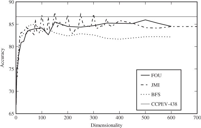
We note that there is no evidence of the curse of dimensionality kicking in within the 700 dimensions we have covered. In fact, both the training and testing error rates appear to stabilise. We also ran a comparison test using all the JPEG-based features (CCPEV-438, FRI-23, Markov-243, HCF-390 and CCCP-54) to see how much trouble the dimensionality can cause. It gave an accuracy of 87.2%, which is better than CCPEV-438, but not significantly so.
Even though automated feature selection does not improve the accuracy, improvements may be found by studying which features are selected. In Table 13.1 we have listed the first 20 features in the order they were selected with the JMI measure. The DCM-243 feature vector is Shi et al.'s Markov-based features subject to difference calibration. As we see, different variations of Markov-based features dominate the list, with a good number of co-occurrence and global histogram features. The single dual histogram feature is the odd one out. Continuing down the list, Markov-based features continue to dominate with local histogram features as a clear number two.
Table 13.1 Top 20 features in the selection according to JMI
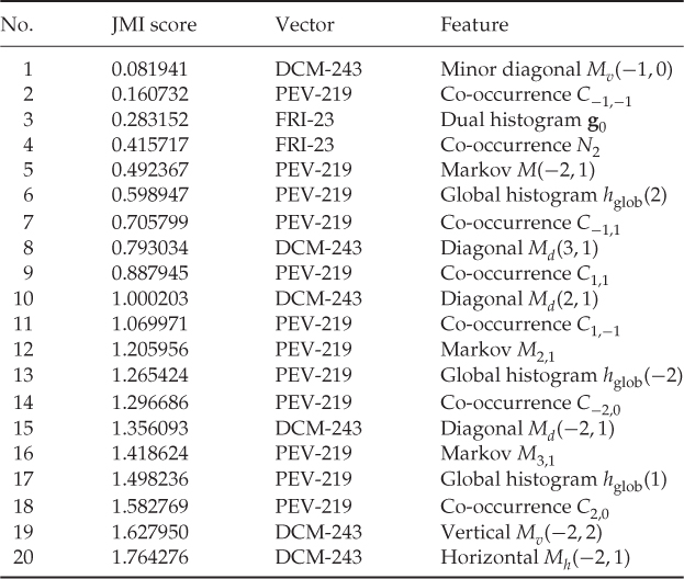
There is no obvious pattern to which individual features are selected from each feature group. Since all of these features are representative of fairly large groups, it is tempting to see if these groups form good feature vectors in their own right. The results are shown in Table 13.2. We note that just the Markov-based features from NCPEV-219 or CCPEV-438 give decent classification, and combining the Markov and co-occurrence features from CCPEV-438, HGS-212 gives a statistically significant improvement in the accuracy with less than half the dimensionality.
Table 13.2 Accuracies for some new feature vectors. Elementary subsets from known feature vectors are listed in the first part. New combinations are listed in the lower part
| Name | Accuracy | Comprises |
| CCPM-162 | 81.9 | Markov features from CCPEV-438 |
| NCPM-81 | 81.0 | Markov features from NCPEV-219 |
| CCCM-50 | 74.5 | Co-occurrence matrix from CCPEV-438 |
| DCCM-25 | 69.5 | Co-occurrence matrix from PEV-219 |
| NCCM-25 | 68.5 | Co-occurrence matrix from NCPEV-219 |
| HGS-162 | 90.3 | |
| HGS-178 | 90.1 | |
| HGS-160 | 90.1 | |
| HGS-180 | 89.9 | |
| HGS-212 | 89.4 | |
| HGS-142 | 88.7 | |
| HGS-131 | 88.2 |
The accuracy can be improved further by including other features as shown in the table. The local histogram features used in HGS-160 and HGS-178 are the ![]() bins from each of the nine frequencies used, taken from NCPEV-219 and CCPEV-438, respectively. Although automated feature selection does not always manage to improve on the accuracy, we have demonstrated that feature selection methods can give very useful guidance to manual selection of feature vectors. Schaathun (2011) also reported consistent results when training and testing the same feature selection with Outguess 0.1 at quality factor 75 and with F5 at quality factor 85.
bins from each of the nine frequencies used, taken from NCPEV-219 and CCPEV-438, respectively. Although automated feature selection does not always manage to improve on the accuracy, we have demonstrated that feature selection methods can give very useful guidance to manual selection of feature vectors. Schaathun (2011) also reported consistent results when training and testing the same feature selection with Outguess 0.1 at quality factor 75 and with F5 at quality factor 85.