Chapter 4

Histogram Analysis

Analysis of the histogram has been used in steganalysis since the beginning, from the simple pairs-of-values or χ² test to analysis of the histogram characteristic function (HCF) and second-order histograms. In this chapter, we will discuss a range of general concepts and techniques using the histogram in the spatial domain. Subsequent chapters will make use of these techniques in other domains.

4.1 Early Histogram Analysis

The histogram was much used in statistical steganalysis in the early days, both in the spatial and the JPEG domains. These techniques were targeted and aimed to exploit specific artifacts caused by specific embedding algorithms. The most well-known example is the pairs-of-values or χ² test, which we discussed in Section 2.3.4.

None of the statistical attacks are difficult to counter. For each and every one, new embedding algorithms have emerged, specifically avoiding the artifact detected. Most instructively, Outguess 0.2 introduced so-called statistics-aware embedding. Sacrificing some embedding capacity, a certain fraction of the coefficients was reserved for dummy modifications designed only to even out the statistics and prevent the (then) known statistical attacks.

A key advantage of machine learning over statistical attacks is that it does not automatically reveal a statistical model to the designer. The basis of any statistical attack is some theoretical model capturing some difference between steganograms and natural images. Because it is well understood, it allows the steganographer to design the embedding to fit the model of natural images, just like the steganalyst can design the attack to detect discrepancies with the model. Machine learning, relying on brute-force computation, gives a model too complex for direct, human analysis. Thus it deprives the steganalyst of some of the insight which could be used to improve the steganographic embedding.

It should be mentioned that more can be learnt from machine learning than what is currently known in the steganalysis literature. One of the motivations for feature selection in Chapter 13 is to learn which features are really significant for the classification and thus get insight into the properties of objects of each class. Further research into feature selection in steganalysis just might provide the insight to design better embedding algorithms, in the same way as insight from statistical steganalysis has improved embedding algorithms in the past.

4.2 Notation

Let I be an image which we view as a matrix of pixels. The pixel value in position (x, y) is denoted as I [x, y]. In the case of colour images, I [x, y] will be a tuple, and we denote the value of colour channel k by I^k [x, y]. We will occasionally, when compactness is required, write I_{x, y} instead of I [x, y].

The histogram of I is denoted by h_I(v). For a grey-scale image we define it as

4.1

where #S denotes the cardinality of a set S. For a colour image we define the histogram for each colour channel k as

We will sometimes use a subscript to identify a steganogram I_s or a cover image I_c. For simplicity, we will write h_s and h_c for their histograms, instead of and .

We define a function δ for any statement E, such that δ(E) = 1 if E is true and δ(E) = 0 otherwise. We will use this to define joint histograms and other histogram-like functions later. As an example, we could define h_I as

which is equivalent to (4.1).

4.3 Additive Independent Noise

A large class of stego-systems can be described in a single framework, as adding an independent noise signal to the image signal. Thus we denote the steganogram I_s as

where I_c is the cover object and X is the distortion, or noise, caused by steganographic embedding. As far as images are concerned, I_s, I_c and X are M × N matrices, but this framework may extend to one-dimensional signals such as audio signals. We say that X is additive independent noise when X is statistically independent of the cover I_c, and each sample X [i, j] is identically and independently distributed.

The two most well-known examples of stego-systems with additive independent noise are spread-spectrum image watermarking (SSIS) and LSB matching. In SSIS (Marvel et al., 1999), this independent noise model is explicit in the algorithm. The message is encoded as a Gaussian signal independently of the cover, and then added to the cover. In LSB matching, the added signal X is statistically independent of the cover, even though the algorithm does calculate X as a function of I_c. If the message bit is 0, the corresponding pixel I_c [i, j] is kept constant if it is even, and changed to become even by adding ± 1 if it is odd. For a message bit equal to one, even pixels are changed while odd pixels are kept constant. The statistical independence is obvious by noting that the message bit is 0 or 1 with 50/50 probability, so that regardless of the pixel value, we have probabilities (25%, 50%, 25%) for X_{i, j} ∈ { − 1, 0, + 1}.

The framework is also commonly used on other embedding algorithms, where X and I_c are statistically dependent. This is, for instance, the case for LSB replacement, where X_{i, j} ∈ {0, + 1} if I_c[i, j] is even, and X_{i, j} ∈ { − 1, 0} otherwise. Even though X is not independent of I_c, it should not be surprising if it causes detectable artifacts in statistics which are designed to detect additive independent noise. Hence, the features we are going to discuss may very well apply to more stego-systems than those using additive independent noise, but the analysis and justifications of the features will not apply directly.

4.3.1 The Effect of Noise

Many authors have studied the effect of random independent noise. Harmsen and Pearlman (2003) and Harmsen (2003) seem to be the pioneers, and most of the following analysis is based on their work. Harmsen's original attack is probably best considered as a statistical attack, but it is atypical in that it targets a rather broad class of different embedding algorithms. Furthermore, the statistics have subsequently been used in machine learning attacks.

Considering the steganogram I_s = I_c + X, it is clear that I_s and I_c have different distributions, so that it is possible, at least in theory, to distinguish statistically between steganograms and clean images. In particular, I_s will have a greater variance, since

and . To make the embedding imperceptible, X will need to have very low variance compared to I_c. The objective is to define statistics which can pick up this difference in distribution.

The proof follows trivially from the definition of convolution, which we include for completeness.

The relationship between the histograms is easier to analyse in the frequency domain. This follows from the well-known Convolution Theorem (below), which is valid in the discrete as well as the continuous case.

Theorem 4.3.3 (Convolution Theorem)

Given two functions f(x) and g(x), and their Fourier transforms F(ω) and G(ω), if then the Fourier transform of h(x) is given as H(ω) = F(ω) · G(ω) for each ω.

---

Theorem 4.3.1 tells us that the addition of independent noise acts as a filter on the histogram. In most cases, the added noise is Gaussian or uniform, and its probability mass function (PMF) forms a low-pass filter, so that it will smooth high-frequency components in the PMF while keeping the low-frequency structure. Plotting the PMFs, the steganogram will then have a smoother curve than the cover image.

Obviously, we cannot observe the PMF or probability distribution function (PDF), so we cannot apply Theorem 4.3.1 directly. The histogram is an empirical estimate for the PMF, as the expected value of the histogram is . Many authors have argued that Theorem 4.3.1 will hold approximately when the histogram h(x) is substituted for f(x). The validity of this approximation depends on a number of factors, including the size of the image. We will discuss this later, when we have seen a few examples.

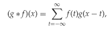
In Figure 4.1, we see the histogram of a cover image and steganograms created at full capacity with LSB and LSB±. It is not very easy to see, but there is evidence, especially in the range 50 ≤ x ≤ 100, that some raggedness in the cover image is smoothed by the additive noise.

Figure 4.1 Sample histograms for clean images and steganograms, based on the ‘beach’ image: (a) cover image; (b) LSB replacement; (c) LSB matching

It is well known that never-compressed images will tend to have more ragged histograms than images which have been compressed, for instance with JPEG. However, as our never-compressed sample shows, the raggedness is not necessarily very pronounced. Harmsen (2003) had examples where the histogram was considerably more ragged, and the smoothing effect of the noise became more pronounced. Evidently, he must have used different image sources; in the sample we studied, the cover images tended to have even smoother histograms than this one.

The smoothing effect can only be expected to be visible in large images. This is due to the laws of large numbers, implying that for sufficiently large samples, the histograms are good approximations for the PMF, and Theorem 4.3.1 gives a good description of the histograms. For small images, the histogram will be ragged because of the randomness of the small sample, both for the steganogram and for the cover. In such a case one will observe a massive difference between the actual histogram of the steganogram and the histogram estimated using Theorem 4.3.1.

4.3.2 The Histogram Characteristic Function

The characteristic function (CF) is the common transform for studying probability distributions in the frequency domain. It is closely related to the Fourier transform. The CF of a stochastic variable X is usually defined as

where f_X is the PMF and i is the imaginary unit solving x² = − 1. The discrete Fourier transform (DFT), however would be

The relevant theoretical properties are not affected by this change of sign. Note in particular that . One may also note that ϕ(u) is the inverse DFT. In the steganalysis literature, the following definition is common.

Combining Theorems 4.3.1 and 4.3.3, we note that H_s(ω) = H_c(ω) · H_x(ω) where H_s, H_c and H_x are the HCF of, respectively, the steganogram, the cover and the embedding distortion.

Theoretical support for using the HCF rather than the histogram in the context of steganalysis was given by Xuan et al. (2005a). They compared the effect of embedding on the PDF and on its Fourier transform or characteristic function, and found that the characteristic function was more sensitive to embedding than the PDF itself.

4.3.3 Moments of the Characteristic Function

Many authors have used the so-called HCF moments as features for steganalysis. The concept seems to have been introduced first by Harmsen (2003), to capture the changes in the histogram caused by random additive noise. The following definition is commonly used.

The use of the term ‘moment’ in steganalysis may be confusing. We will later encounter statistical moments, and the moments of a probability distribution are also well known. The characteristic function is often used to calculate the moments of the corresponding PDF. However, the HCF moments as defined above seem to be unrelated to the more well-known concept of moments. On the contrary, if we replace H by the histogram h in the definition of m_n, we get the statistical moments of the pixel values.

def hcfmoments(im,order=1):
   """Calculate the HCF moments of the
   given orders for the image im."""
   h = np.histogram( h, range(257) )
   H0 = np.fft.fft(h)
   H = np.abs( H0[1:129] )
   M = sum( [ (float(k)/(256))**order*H[k] for k in xrange(128) ] )
   S = np.sum(H)
   return M / S

Because the histogram h(x) is real-valued, is symmetric, making the negative frequencies redundant, which is why we omit them in the sums. Most authors include the zero frequency H(0) in the sum, but Shi et al. (2005a) argue that, because this is just the total number of pixels in the image, it is unaffected by embedding and may make the moment less sensitive.

The HCF-COM m₁ was introduced as a feature by Harmsen (2003), and has been used by many authors since. We will study it in more detail. Code Example 4.1 shows how it can be calculated in Python, using the FFT and histogram functions from numpy. Let C(I) = m₁ denote the HCF-COM of an arbitrary image I. The key to its usefulness is the following theorem.

Theorem 4.3.6 (Harmsen and Pearlman, 2003)

For an embedding scheme with non-increasing for k = 0, 1, … , N − 1, the HCF-COM decreases or remains the same after embedding, i.e.

with equality if and only if for all k.

---

The proof depends on the following version of ebyšev's¹ inequality. Because this is not the version most commonly found in the literature, we include it with a proof based on Hardy et al. (1934).

---

Proof

We consider the difference between the left- and right-hand side of the inequality, and write

Note that for any index pair (i, j) included in the sum, (j, i) is also included. Therefore, we can write

Since a_i and b_i are oppositely ordered, a_i − a_j and b_j − b_i have the same sign. With p_i ≥ 0, we thus get that D ≥ 0. If, on the contrary, a_i and b_i are similarly ordered, we get .

---

---

Proof of Theorem 4.3.6

Since is non-increasing in k and is non-negative for all k, we can use a_k = k, and in Lemma 4.3.7 to get that

4.3

Rearranging terms, we get

4.4

It is easy to see that equality holds in (4.3), and hence in (4.4), if is constant in k. Then, note that H_X(k = 0) = 1 because H_X is the Fourier transform of a PMF which has to sum to 1. Since H_X(k) is also non-increasing, we note that equality can only hold if for all k.

---

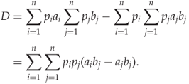
In Figure 4.2 we can see the empirical HCF-COM plotted as a function of the length of the embedded message, using LSB matching for embedding. On the one hand, this confirms Theorem 4.3.6; HCF-COM is smaller for steganograms than it is for the corresponding cover image. On the other hand, the difference caused by embedding is much smaller than the difference between different cover images. Thus, we cannot expect HCF-COM to give a working classifier as a sole feature, but it can quite possibly be useful in combination with others.

Figure 4.2 Plot of HCF-COM for different test images and varying message lengths embedded with LSB matching. We show plots for both the high-resolution originals: (a) and the low-resolution grey-scale images; (b) that we use for most of the tests

We note that the high-resolution image has a much smoother and more consistently declining HCF-COM. This is probably an effect of the laws of large numbers; the high-resolution image has more samples and thus the random variation becomes negligible.

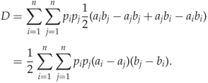
We have also made a similar plot using LSB replacement in Figure 4.3. Notably, HCF-COM increases with the message length for LSB replacement. This may come as a surprise, but it demonstrates that the assumption of random independent noise is critical for the proof of Theorem 4.3.6. In contrast, the effect of LSB replacement on HCF-COM seems to be greater than that of LSB matching, so it is not impossible that HCF-COM may prove useful as a feature against LSB replacement.

Figure 4.3 Plot of HCF-COM for varying message lengths with LSB replacement

As we shall see throughout the book, the HCF moments have been used in many variation for steganalysis, including different image representations and higher-order moments as well as HCF-COM.

4.3.4 Amplitude of Local Extrema

Zhang et al. (2007) proposed a more straight forward approach to detect the smoothing effect of additive noise. Clean images very often have narrow peaks in the histogram, and a low-pass filter will tend to have a very pronounced effect on such peaks. Consider, for instance, a pixel value x which is twice as frequent as either neighbour x ± 1. If we embed with LSB matching at full capacity, half of the x pixels will change by ± 1. Only a quarter of the x ± 1 pixels will change to exactly x, and this is only half as many. Hence, the peak will be, on average, 25% lower after embedding.

In Zhang et al.'s (2007) vocabulary, these peaks are called local extrema; they are extreme values of the histogram compared to their local neighbourhood. They proposed a way to measure the amplitude of the local extrema (ALE). In symbolic notation, the local extrema is the set defined as

4.5

def alepts(h,S):
     """Return a list of local extrema on the histogram h
     restricted to the set S."""
     return [ x for x in S
                 if (h[x] − h[x−1])*(h[x] − h[x+1]) > 0 ]
def alef0(h,E):
     "CalculateALEbasedonthelistEoflocalextrema."
     return sum( [ abs(2*h[x] − h[x−1] − h[x+1]) for x in E ] )
def ale1d(I):
   (h,b) = np.histogram(I.flatten(),bins=list(xrange(257)))
   E1 = alepts(xrange(3,253))
   f1 = alef0(h,E1)
   E2 = alepts([1,2,253,254])
   f2 = alef0(h,E2)
   return [f1,f2]

For 8-bit images, , as the condition in (4.5) would be undefined for x = 0, 255. The basic ALE feature, introduced by Zhang et al. (2007), is defined as

4.6

The ragged histogram is typical for images that have never been compressed, and the experiments reported by Zhang et al. (2007) show that f₀ is very effective for never-compressed images, but considerably less discriminant for images that have ever been JPEG compressed.

Irregular effects occur in the histogram close to the end points. The modification of LSB matching is ± 1 with uniform distribution, except at 0 and 255. A zero can only change to one, and 255 only to 254. Because of this, Cancelli et al. (2008) proposed, assuming 8-bit grey-scale images, to restrict . The resulting modified version of f₀ thereby ignores values which are subject to the exception occurring at 0 and 255. To avoid discarding the information in the histogram at values 1, 2, 253, 254, they define a second feature on these points. Thus, we get two first-order ALE features as follows:

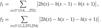
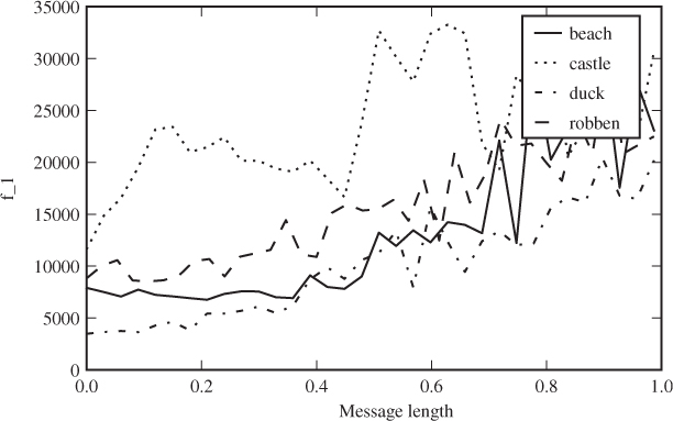
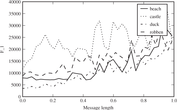
Python definitions of these features are shown in Code Example 4.2. In Figure 4.4 we can see how f₁ depends on the embedded message length for a couple of sample images. The complete set of ALE features (ALE-10) also includes second-order features, which we will discuss in Section 4.4.2.

Figure 4.4 The ALE feature f₁ as a function of the message length for a few sample images with LSB replacement. The message length is given as a fraction of capacity

4.4 Multi-dimensional Histograms

So far, we have discussed HCF-COM as if we were going to apply it directly to grey-scale images, but the empirical tests in Figures 4.2 and 4.3 show that this is unlikely to give a good classifier. In order to get good accuracy, we need other features. There are indeed many different ways to make effective use of the HCF-COM feature, and we will see some in this section and more in Chapter 9.

Theorem 4.3.1 applies to multi-dimensional distributions as well as one-dimensional ones. Multi-dimensional distribution applies to images in at least two different ways. Harmsen and Pearlman (2003) considered colour images and the joint distribution of the colour components in each pixel. This gives a three-dimensional distribution and a 3-D (joint) histogram. A more recent approach, which is also applicable to grey-scale images, is to study the joint distribution of adjacent pixels.

The multi-dimensional histograms capture correlation which is ignored by the usual one-dimensional histogram. Since pixel values are locally dependent, while the noise signal is not, the multi-dimensional histograms will tend to give stronger classifiers. Features based on the 1-D histogram are known as first-order statistics. When we consider the joint distribution of n pixels, we get nth-order statistics.

It is relatively easy to build statistical models predicting the first-order features, and this enables the steganographer to adapt the embedding to keep the first-order statistics constant under embedding. Such statistics-aware embedding was invented very early, with Outguess 0.2. Higher-order models rapidly become more complex, and thus higher-order statistics (i.e. n > 1) are harder to circumvent.

4.4.1 HCF Features for Colour Images

Considering a colour image, there is almost always very strong dependency between the different colour channels. Look, for instance, at the scatter plots in Figure 4.5. Each point in the plot is a pixel, and its coordinates (x, y) represent the value in two different colour channels. If the channels had been independent, we would expect an almost evenly grey plot. As it is, most of the possible combinations hardly ever occur. This structure in the joint distribution is much more obvious than the structure in the one-dimensional histogram. Thus, stronger classifiers can be expected.

Figure 4.5 Scatter plots showing the correlation between two colour channels: (a) red/green; (b) red/blue. The plots are based on the ‘castle’ image, scaled down to 512 × 343

The joint distribution of pixel values across three colour channels can be described as a three-dimensional (joint) histogram

The only difference between this definition and the usual histogram is that the 3-D histogram is a function of three values (u, v, w) instead of one. Theorem 4.3.6 can easily be generalised for joint probability distributions, as a multi-dimensional convolution. Thus, the theory we developed in the 1-D case should apply in the multi-dimensional case as well.

The multi-dimensional HCF is a multi-dimensional Fourier transform of the joint histogram, and the HCF centre of mass can be generalised as follows.

Definition 4.4.1

The generalised centre of mass of a d-dimensional HCF is a d-tuple given by

and . Each element c_i of is sometimes called a marginal moment of order 1.

---

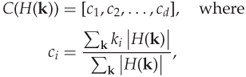
Having generalised all the concepts for multi-dimensional distributions, we let H³(k, l, m) denote the HCF obtained as the 3-D DFT of h_I(u, v, w). The feature vector of Harmsen and Pearlman (2003), which we denote as HAR3D-3, is a three-dimensional vector defined as C(H³(k, l, m)). For comparison, we define HAR1D-3 to be the HCF-COM calculated separately for each colour channel, which also gives a 3-D feature vector.

The disadvantage of HAR3D-3 is that it is much slower to calculate (Harmsen et al., 2004) than HAR1D-3. The complexity of the d-D DFT algorithm is O(N^dlogN) where the input is an array of N^d elements. Thus, for 8-bit images, where N = 256, HAR1D-3 is roughly 20 000 times faster to compute compared with HAR3D-3.

A compromise between HAR1D-3 and HAR3D-3 is to use the 2-D HCF for each pair of colour channels. For each of the three 2-D HCFs, the centre of mass C(H(k₁, k₂)) is calculated. This gives two features for each of three colour pairs. The result is a 6-D feature vector which we call HAR2D-6. It is roughly 85 times faster to compute than HAR3D-3 for 8-bit images. Both Harmsen et al. (2004) and Ker (2005a) have run independent experiments showing that HAR2D-6 has accuracy close to HAR3D-3, whereas HAR1D-3 is significantly inferior.

def har2d(I):
   "ReturntheHAR2D−6featurevectorofIasalist."
   (R,G,B) = (I[:,:,0],I[:,:,1],I[:,:,2])
   return hdd((R,B)) + hdd((R,G)) + hdd((B,G))
def hdd(L):
   """
   Given a list L of 8−bit integer arrays, return the HCF−COM
   based on the joint histogram of the elements of L.
   """
   bins = tuple([ list(xrange(257)) for i in L ])
   L = [ X.flatten() for X in L ]
   (h,b) = np.histogramdd( L, bins=bins )
   H = np.fft.fftn(h)
   return hcom(H)
def hcom(H1):
   "Calculatethecentreofmassofa2−DHCFH."
   H = H1[0:129,0:129]
   S = np.sum(H)
   return [ hcfm( np.sum(H,1) )/S, hcfm( np.sum(H,0) )/S ]

Code Example 4.3 shows how to calculate HAR2D-6: har2d calculates the feature vector from an image, using hdd() to calculate the HCF centre of mass from a given pair of colour channels, which in turn uses hcom to calculate the centre of mass for an arbitrary HCF.

4.4.2 The Co-occurrence Matrix

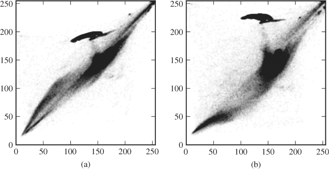
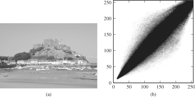
For grey-scale images the previous section offers no solution, and we have to seek higher-order features within a single colour channel. The first-order features consider pixels as if they were independent. In reality, neighbouring pixels are highly correlated, just like the different colour channels are. The scatter plot in Figure 4.6 is analogous to those showing colour channels. We have plotted all the horizontal pixel pairs (x, y) = (I [i, j], I [i, j + 1]) of a grey-scale image. Dark colour indicates a high density of pairs, and as we can see, most of the pairs cluster around the diagonal where I [i, j] ≈ I [i, j + 1]. This is typical, and most images will have similar structure. Clearly, we could consider larger groups of pixels, but the computational cost would then be significant.

Figure 4.6 Image (a) with its horizontal co-occurrence scatter diagram (b)

Numerically, we can capture the distribution of pixel pairs in the co-occurrence matrix. It is defined as the matrix , where

We are typically interested in the co-occurrence matrices for adjacent pairs, that is M_{i, j} for i, j = − 1, 0, + 1, but there are also known attacks using pixels at distance greater than 1. The co-occurrence matrix is also known as the second-order or 2-D histogram. An example of how to code it in Python is given in Code Example 4.4.

Code Example 4.4 : Calculate the co-occurrence matrix of C in the given direction d1,d2

def cooccurrence(C,(d1,d2)):
     (C1,C2) = splitMatrix(C,(d1,d2))
     (h,b) = np.histogram2d( C1.flatten(),C2.flatten(),
           bins=range(0,257 )
     return h
def splitMatrix(C,(d1,d2)):
     """Return the two submatrices of C as needed to calculate
     co-occurrence matrices."""
     return (sm(C,d1,d2),sm(C,−d1,−d2))
def sm(C,d1,d2):
     "AuxiliaryfunctionforsplitMatrix()."
     (m,n) = C.shape
     (m1,m2) = (max(0,−d1), min(m,m−d1))
     (n1,n2) = (max(0,−d2), min(n,n−d2))
     return C[m1:m2,n1:n2]

---

Sullivan's Features

Additive data embedding would tend to make the distribution more scattered, with more pairs further from the diagonal in the scatter plot. This effect is exactly the same as the one we discussed with respect to the 1-D histogram, with the low-pass filter caused by the noise blurring the plot. The co-occurrence matrix M_s of a steganogram will be the convolution M_c * M_X of the co-occurrence matrices M_c and M_X of the cover image and the embedding distortion. The scattering effect becomes very prominent if the magnitude of the embedding is large. However, with LSB embedding, and other techniques adding ± 1 only, the effect is hardly visible in the scatter plot, but may be detectable statistically or using machine learning.

Sullivan et al. (2005) suggested a simple feature vector to capture the spread from the diagonal. They used a co-occurrence matrix M = [m_{i, j}] of adjacent pairs from a linearised (1-D) sequence of pixels, without addressing whether it should be parsed row-wise or column-wise from the pixmap. This, however, is unlikely to matter, and whether we use M = M_{1, 0} or M = M_{0, 1}, we should expect very similar results.

For an 8-bit grey-scale image, M has 2¹⁶ elements, which is computationally very expensive. Additionally, M may tend to be sparse, with most positive values clustering around the main diagonal. To address this problem, Sullivan et al. (2005) used the six largest values m_{k, k} on the main diagonal of M, and for each of them, a further ten adjacent entries

with the convention that m_{k, l} = 0 when the indices go out of bounds, that is for l < 0. This gives 66 features.

Additionally, they used every fourth of the values on the main diagonal, that is

This gives another 64 features, and a total of 130. We will denote the feature vector as SMCM-130.

The SMCM-130 feature vector was originally designed to attack a version of SSIS of Marvel et al. (1999). SSIS uses standard techniques from communications and error-control coding to transmit the steganographic image while treating the cover image as noise. The idea is that the embedding noise can be tailored to mimic naturally occurring noise, such as sensor noise in images. The theory behind SSIS assumes floating-point pixel values. When the pixels are quantised as 8-bit images, the variance of the Gaussian embedding noise has to be very large for the message to survive the rounding errors, typically too large to mimic naturally occurring noise. In the experiments of Marvel et al. using 8-bit images, SSIS becomes very easily detectable. Standard LSB replacement or matching cause much less embedding noise and are thus harder to detect. It is possible that SSIS can be made less detectable by using raw images with 12- or 14-bit pixels, but this has not been tested as far as we know.

The 2-D HCF

To study the co-occurrence matrix in the frequency domain, we can follow the same procedure as we used for joint histograms across colour channels. It applies to any co-occurrence matrix M. The 2-D HCF H²(k, l) is obtained as the 2-D DFT of M.

Obviously, we can form features using the centre of mass from Definition 4.4.1. However, Ker (2005b) used a simpler definition to get a scalar centre of mass from a 2-D HCF. He considered just the sum of the pixels in the pair, and defined a centre of mass as

4.7

where is the 2-D HCF of the co-occurrence matrix M. Obviously, this idea may be extended to use higher-order moments of the sum (i + j) as well. Ker (2005b) used just C₂(M_{0, 1}) as a single discriminant, and we are not aware of other authors who have used 2-D HCFs in this way.

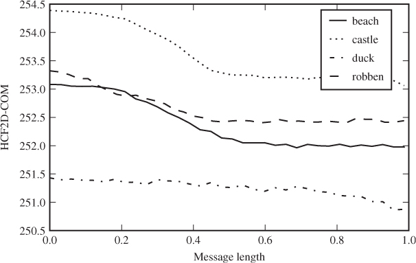
Comparing Figure 4.7 to Figure 4.2, we see that Ker's 2-D HCF-COM feature varies much more with the embedded message length, and must be expected to give a better classifier.

Figure 4.7 Ker's 2-D HCF-COM feature as a function of embedded message length for LSB matching

Amplitude of Local Extrema

The ALE features can be generalised for joint distributions in the same way as the HCF moments. The second-order ALE features are calculated from the co-occurrence matrices, or 2-D adjacency histograms in the terminology of Cancelli et al. (2008).

A local extremum in a 1-D histogram is a point which is either higher or lower than both neighbours. In 2-D, we define a local extremum to be a point where either all four neighbours (above, below, left, right) are higher, or all four are lower. Formally, a local extremum in a co-occurrence matrix M is a point (x, y) satisfying either

4.8

4.9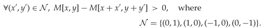

Let be the set of all the local extrema.

A potential problem is a large number of local extrema with only negligible differences in (4.8) or (4.9). Such marginal extrema are not very robust to embedding changes, and ideally we want some robustness criterion to exclude marginal extrema.

It is reasonable to expect the co-occurrence matrix to be roughly symmetric, i.e. M[x, y] ≈ M[y, x]. After all, M[y, x] would be the co-occurrence matrix of the image flipped around some axis, and the flipped image should normally have very similar statistics to the original image. Thus, a robust local extremum (x, y) should be extremal both with respect to M[x, y] and M[y, x]. In other words, we define a set of robust local extrema, as

According to Cancelli et al., this definition improves the discriminating power of the features. Thus, we get a 2-D ALE feature A(M) for each co-occurrence matrix M, defined as follows:

4.10

We use the co-occurrence of all adjacent pairs, horizontally, vertically and diagonally. In other words,

to get four features A(M). Figure 4.8 shows how a second-order ALE feature responds to varying message length.

Figure 4.8 The second-order ALE feature A(M_{0, 1}) as a function of the embedded message length for our test images

The last of the ALE features are based on the ideas discussed in Section 4.4.2, and count the number of pixel pairs on the main diagonal of the co-occurrence matrix:

4.11

When the embedding increases the spreading off the main diagonal as discussed previously, d(M) will decrease.

Code Example 4.5 : Calculate the 2-D ALE features and for the given direction (d₁, d₂)

def ale2d(I,(d1,d2)):
   h = cooccurrence(I,(d1,d2))
   Y = h[1:−1,1:−1]
   L = [h[:−2,1:−1],h[2:,1:−1],h[1:−1,:−2],h[1:−1,2:]]
   T  = reduce( andf, [ ( Y < x ) for x in L ] )
   T |= reduce( andf, [ ( Y > x ) for x in L ] )
   T &= T.transpose()
   A = sum( np.abs(4*Y[T] − sum( [ x[T] for x in L ] )) )
   d = sum( [ h[k,k] for k in xrange(h.shape[0]) ] )
   return [A,d]

---

Code Example 4.5 demonstrates how to calculate ALE features in Python. We define the list L as the four different shifts of I by one pixel up, down, left or right. The Boolean array T is first set to flag those elements of I that are smaller than all their four neighbours, and subsequently or'ed with those elements smaller than the neighbours. Thus, T identifies local extrema. Finally, T is and'ed with its transpose to filter out robust local extrema only. The two features A and d are set using the definitions (4.10) and (4.11).

Cancelli et al. (2008) proposed a 10-D feature vector, ALE-10, comprising the first-order features f₁ and f₂ and eight second-order features. Four co-occurrence matrices M = M_{0, 1}, M_{1, 0}, M_{1, 1}, M_{1, −1} are used, and the two features A(M) and d(M) are calculated for each M, to give the eight second-order features.

4.5 Experiment and Comparison

We will end each chapter in this part of the book with a quick comparison of accuracies on grey-scale images, between feature vectors covered so far. Table 4.1 shows the performance of ALE-10 and SMCM-130. We have not considered colour image or single features in this test. Neither of the feature vectors is able to detect very short messages, but both have some discriminatory power for longer messages.

Table 4.1 Comparison of accuracies of feature vectors discussed in this chapter

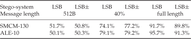
The SMCM features do badly in the experiments, especially considering the fact that they have high dimensionality. This makes sense as the SMCM features consider the diagonal elements of the co-occurrence matrix separately, where each element would be expected to convey pretty much the same information.

¹ Also spelt Chebyshev or Tchebychef.