Chapter 12

Other Classification Algorithms

The problem of classification can be approached in many different ways. The support vector machine essentially solves a geometric problem of separating points in feature space. Probability never entered into the design or training of SVM. Probabilities are only addressed when we evaluate the classifier by testing it on new, unseen objects.

Many of the early methods from statistical steganalysis are designed as hypothesis tests and follow the framework of sampling theory within statistics. A null hypothesis H₀ is formed in such a way that we have a known probability distribution for image data assuming that H₀ is true. For instance, ‘image I is a clean image’ would be a possible null hypothesis. This gives precise control of the false positive rate. The principle of sampling theory is that the experiment is defined before looking at the observations, and we control the risk of falsely rejecting H₀ (false positives). The drawback of this approach is that this p-value is completely unrelated to the probability that H₀ is true, and thus the test does not give us any quantitative information relating to the problem.

The other main school of statistics, along side sampling theory, is known as Bayesian statistics or Bayesian inference. In terms of classification, Bayesian inference will aim to determine the probability of a given image I belonging to a given class C a posteriori, that is after considering the observed image I.

It is debatable whether SVM and statistical methods are learning algorithms. Some authors restrict the concept of machine learning to iterative and often distributed methods, such as neural networks. Starting with a random model, these algorithms inspect one training object at a time, adjusting the model for every observation. Very often it will have to go through the training set multiple times for the model to converge. Such systems learn gradually over time, and in some cases they can continue to learn also after deployment. At least new training objects can be introduced without discarding previous learning. The SVM algorithm, in contrast, starts with no model and considers the entire training set at once to calculate a model. We did not find room to cover neural networks in this book, but interested readers can find accessible introductions in books such as, for instance, Negnevitsky (2005) or Luger (2008).

In this chapter, we will look at an assortment of classifier algorithms. Bayesian classifiers, developed directly from Bayesian statistics, fit well into the framework already considered, of supervised learning and classification. Regression analysis is also a fundamental statistical technique, but instead of predicting a discrete class label, it predicts a continuous dependent variable, such as the length of the embedded message. Finally, we will consider unsupervised learning, where the machine is trained without knowledge of the true class labels.

12.1 Bayesian Classifiers

We consider an observed image I, and two possible events C_S that I be a steganogram and C_C that I be a clean image. As before, we are able to observe some feature vector F(I) = (F₁(I), … , F_N(I)). The goal is to estimate the a posteriori probability for C = C_C, C_S. This can be written using Bayes' law, as

12.1

The a priori probability is the probability that I is a steganogram, as well as we can gauge it, before we have actually looked at I or calculated the features . The a posteriori probability , similarly, is the probability after we have looked at I. The final two elements, and , describe the probability distribution of the features over a single class and over all images respectively. Note that (12.1) is valid whether is a PMF or a PDF.

The Bayesian classifier is as simple as estimating using (12.1), and concluding that the image is a steganogram if , or equivalently if

12.2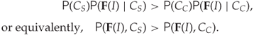

This, however, is not necessarily simple. The probability distribution of must be estimated, and we will discuss some relevant methods below. The estimation of the a priori probability is more controversial; it depends heavily on the application scenario and is likely to be subjective.

The explicit dependence on is a good thing. It means that the classifier is tuned to the context. If we employ a steganalyser to monitor random images on the Internet, must be expected to be very small, and very strong evidence from is then required to conclude that the image is a steganogram. If the steganalyser is used where there is a particular reason to suspect a steganogram, will be larger, and less evidence is required to conclude that I is more likely a steganogram than not.

On the contrary how do we know what is for a random image? This will have to rely on intuition and guesswork. It is customary to assume a uniform distribution, , if no information is available, but in steganalysis we will often find ourselves in the position where we know that is far off, but we have no inkling as to whether or is closer to the mark.

12.1.1 Classification Regions and Errors

The classification problem ultimately boils down to identifying disjoint decision regions , where we can assume that I is a steganogram for all and a clean image for all . It is possible to allow points , which would mean that both class labels are equally likely for image and we refuse to make a prediction. For simplicity we assume that , so that a prediction will be made for any image .

In Figure 12.1 we show an example plot of and for a one-dimensional feature vector. The decision regions and will be subsets of the -axis. The Bayes decision rule would define and so that every point in the feature space would be associated with the class corresponding to the higher curve. In the plot, that means is the segment to the left of the vertical line and is the segment to the right.

Figure 12.1 Feature probability distribution for different classes

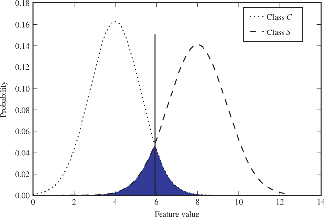
The shaded area represents the classification error probability , or Bayes' error, which can be defined as the integral

12.3

If we move the boundary between the decision regions to the right, we will get fewer false positives, but more false negatives. Similarly, if we move it to the left we get fewer false negatives at the expense of false positives. Either way, the total error probability will increase. One of the beauties of the Bayes classifier is its optimality, in the sense that it minimises the probability of classification error. This is not too hard to prove, as we shall see below.

Theorem 12.1.1

The Bayes classification rule minimises the probability of classification error.

---

---

Proof

The decision rule in (12.2) defines two decision regions and , so that when (12.2) is satisfied and otherwise. To minimise the expression in (12.3), and must be chosen such that every point appears in the integral with the smaller integrand, that is

which is exactly the Bayes decision rule.

---

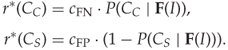
12.1.2 Misclassification Risk

Risk captures both the probability of a bad event and the degree of badness. When different types of misclassification carry different costs, risk can be a useful concept to capture all error types in one measure. False positives and false negatives are two different bad events which often carry different costs. We are familiar with the error probabilities and , and we introduce the costs and .

The risk associated with an event is commonly defined as the product of the probability and cost. In particular, the risk of a false positive can be defined as

12.4

where denotes the event that we intercept a clean image. Similarly, the risk of a false negative would be

12.5

The total risk of a classifier naturally is the sum of the risks associated with different events, i.e.

12.6

In this formulation, we have assumed for simplicity that there is zero cost (or benefit) associated with correct classifications. It is often useful to add costs or benefits and in the event of correct positive and negative classification, respectively. Often and will be negative.

It is important to note that the cost does not have to be a monetary value, and there are at least two reasons why it might not be. Sometimes non-monetary cost measures are used because it is too difficult to assign a monetary value. Other times one may need to avoid a monetary measure because it does not accurately model the utility or benefit perceived by the user. Utility is an economic concept used to measure subjective value to an agent, that is Wendy in our case. One important observation is that utility does not always scale linearly in money. Quite commonly, individuals will think that losing £1000 is more than a hundred times worse than losing £10. Such a sub-linear relationship makes the user risk averse, quite happy to accept an increased probability of losing a small amount if it also reduces the risk of major loss.

In order to use risk as an evaluation heuristic for classifiers, we need to estimate and so that they measure the badness experienced by Wendy in the event of misclassification. The misclassification risk can be written as

assuming zero cost for correct classification.

We can define an a posteriori risk as well:

It is straightforward to rework the Bayesian decision rule to minimise the a posteriori risk instead of the error probability.

12.1.3 The Naïve Bayes Classifier

The Bayes classifier depends on the probability distribution of feature vectors. For one-dimensional feature vectors, this is not much of a problem. Although density estimation can be generalised for arbitrary dimension in theory, it is rarely practical to do so. The problem is that accurate estimation in high dimensions requires a very large sample, and the requirement grows exponentially.

The naïve Bayes classifier is a way around this problem, by assuming that the features are statistically independent. In other words, we assume that

12.7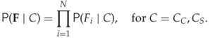

This allows us to simplify (12.1) to

12.8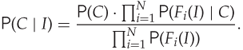

Thus, we can estimate the probability distribution of each feature separately, using one-dimensional estimation techniques.

Of course, there is a reason that the classifier is called naïve Bayes. The independence assumption (12.7) will very often be false. However, the classifier has proved very robust to violations of the independence assumption, and in practice, it has proved very effective on many real-world data sets reported in the pattern recognition literature.

12.1.4 A Security Criterion

The Bayes classifier illustrates the fundamental criterion for classification to be possible. If the probability distribution of the feature vector is the same for both classes, that is, if

12.9

the Bayes decision rule will simply select the a priori most probable class, and predict the same class label regardless of the input. If there is no class skew, the output will be arbitrary.

The difference between the two conditional probabilities in (12.9) is a measure of security; the greater the difference, the more detectable is the steganographic embedding. A common measure of similarity of probability distributions is the relative entropy.

Definition 12.1.2

The relative entropy (aka. Kullback–Leibler divergence) between two (discrete) probability distributions and is defined as

Note that the definition is only valid if for all such that .

---

We have , with equality if and only if the two distributions are equal. The relative entropy is often thought of as a distance, but it is not a distance (or metric) in the mathematical sense. This can easily be seen by noting that is not in general equal to .

Cachin (1998) suggested using the relative entropy to quantify the security of a stego-system. Since security is an absolute property, it should not depend on any particular feature vector, and we have to consider the probability distribution of clean images and steganograms.

Definition 12.1.3 (Cachin, 1998)

Consider a stego-system and let be a cover and a steganogram. Both and are considered as stochastic variables drawn from some set of possible images. We say that is -secure against a passive warden if

If , the stego-system is perfectly secure.

---

Theorem 12.1.4

If a stego-system is -secure, any steganalytic attack with false positive probability and false negative probability will satisfy

12.10

---

---

Proof

The steganalysis attack can be considered as a mapping of one random variable, namely the image , into a Boolean stochastic variable which is either ‘stego’ or ‘clean’. A standard result in information theory says that such deterministic processing cannot increase the relative entropy. Hence

where and are the probability distributions of the predicted class label for clean images and steganograms respectively.

The right-hand side of (12.10) is just the binary relative entropy, sometimes denoted , where and are binary stochastic variables with probability distributions and respectively.

---

Cachin's security criterion high lights a core point in steganography and steganalysis. Detectability is directly related to the difference between the probability distributions of clean images and steganograms. This difference can be measured in different ways; as an alternative to the Kullback–Leibler divergence, Filler and Fridrich (2009a,b) used Fisher information. In theory, Alice's problem can be described as the design of a cipher or stego-system which mimics the distribution of clean images, and Wendy's problem is elementary hypothesis testing.

In practice, the information theoretic research has hardly led to better steganalysis nor steganography. The problem is that we are currently not able to model the probability distributions of images. If Alice is not able to model , she cannot design an -secure stego-system. In contrast, if Wendy cannot model either, Alice probably does not need a theoretically -secure stego-system.

12.2 Estimating Probability Distributions

There are at least three major approaches to estimating probability density functions based on empirical data. Very often, we can make reasonable assumptions about the shape of the PDF, and we only need to estimate parameters. For instance, we might assume the distribution is normal, in which case we will only have to estimate the mean and variance in order to get an estimated probability distribution. This is easily done using the sample mean and sample variance .

If we do not have any assumed model for the PDF, there are two approaches to estimating the distributions. The simplest approach is to discretise the distribution by dividing into a finite number of disjoint bins and use the histogram. The alternative is to use a non-parametric, continuous model. The two most well-known non-parametric methods are kernel density estimators, which we will discuss below, and nearest neighbour.

12.2.1 The Histogram

Let be a stochastic variable drawn from some probability distribution on some continuous space . We can discretise the distribution by defining a discrete random variable as

The probability mass function of is easily estimated by the histogram of the observations of .

We can view the histogram as a density estimate, by assuming a PDF which is constant within each bin:

where is the number of observations and is the width (or volume) of the bin . If the sample size is sufficiently large, and the bin widths are wisely chosen, then will indeed be a good approximation of the true PDF of . The challenge is to select a good bin width. If the bins are too wide, any high-frequency variation in will be lost. If the bins are too narrow, each bin will have very few observations, and will be dominated by noise caused by the randomness of observations. In the extreme case, most bins will have zero or one element, with many empty bins. The result is that is mainly flat, with a spike wherever there happens to be an observation.

There is no gospel to give us the optimal bin size, and it very often boils down to trial and error with some subjective evaluation of the alternatives. However, some popular rules of thumb exist. Most popular is probably Sturges' rule, which recommends to use bins, where is the sample size. Interested readers can see Scott (2009) for an evaluation of this and other bin size rules.

12.2.2 The Kernel Density Estimator

Finally, we shall look at one non-parametric method, namely the popular kernel density estimator (KDE). The KDE is sometimes called Parzen window estimation, and the modern formulation is very close to the one proposed by Parzen (1962). The principles and much of the theory predates Parzen; see for instance Rosenblatt (1956), who is sometimes co-credited for the invention of KDE.

The fundamental idea in KDE is that every observation is evidence of some density in a certain neighbourhood around . Thus, should make a positive contribution to for all and a zero contribution for . The KDE adds together the contributions of all the observations .

The contribution made by each observation can be modelled as a kernel function , where

Summing over all the observations, the KDE estimate of the PDF is defined as

12.11

To be a valid PDF, has to integrate to 1, and to ensure this, we require that the kernel also integrates to one, that is

It is also customary to require that the kernel is symmetric around , that is . It is easy to verify that if is non-negative and integrates to 1, then so does as defined in (12.11). Hence, is a valid probability density function. Note that the kernel functions used here are not necessarily compatible with the kernels used for the kernel trick in Chapter 11, although they may sometimes be based on the same elementary functions, such as the Gaussian.

The simplest kernel is a hypercube, also known as a uniform kernel, defined as

where is the dimensionality of . The uniform kernel, which assigns a constant contribution to the PDF within the neighbourhood, will make a PDF looking like a staircase. To make a smoother PDF estimate, one would use a kernel function which is diminishing in the distance from the origin. Alongside the uniform kernel, the Gaussian kernel is the most commonly used. It is given by

and will give a much smoother PDF estimate.

The kernel density estimate is sensitive to scaling. This is easy to illustrate with the uniform kernel. If the sample space is scaled so that the variance of the observations increases, then fewer observations will fall within the neighbourhood defined by the kernel. We would get the same effect as with a histogram with a very small bin width. Most bins or neighbourhoods are empty, and we get a short spike in wherever there is an observation. In the opposite extreme, where the observations have very low variance, the PDF estimate would have absolutely no high-frequency information. In order to get a realistic estimate we thus need to scale either the kernel or the data in a way similar to tuning the bin width of a histogram.

The KDE analogue of the bin width is known as the bandwidth. The scaling can be incorporated into the kernel function, by introducing the so-called scaled kernel

where the bandwidth scales the argument to . It is easily checked that if integrates to 1, then so does , thus can replace in the KDE definition (12.11). In the previous discussion, we related the scaling to the variance. It follows that the bandwidth should be proportional to the standard deviation so that the argument to the kernel function has fixed variance.

from scipy.stats.kde import gaussian_kde as gkde
import numpy as np
import matplotlib.pyplot as plt
S = np.random.randn( int(opt.size) )
X = [ i*0.1 for i in xrange(−40,40) ]
kde = gkde(S)   # Instantiate estimator
Y = kde(X)       # Evaluate estimated PDF
plt.plot( X, Y, "k−." )

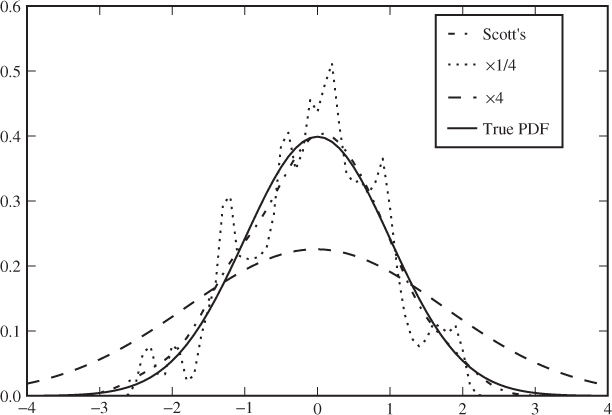
The effect of changing bandwidth is illustrated in Figure 12.2. Scott's rule dictates a bandwidth of

where is the sample standard deviation. We can see that this gives a rather good estimate in the figure. If the bandwidth is reduced to a quarter, we see significant noise, and if it is four times wider, then the estimated PDF becomes far too flat. Code Example 12.1 shows how a KDE can be computed using the standard scipy library in Python. Only the Gaussian kernel is supported, and unfortunately, the bandwidth can only be changed by modifying the source code.

Figure 12.2 Examples of Gaussian KDE estimates from 100 pseudo-random points from a standard normal distribution

In the multivariate case , there is no reason to expect the same bandwidth to be optimal in all dimensions. To scale the different axes separately, we use a bandwidth matrix instead of the scalar bandwidth , and the scaled kernel can be written as

12.12

where denotes the determinant of . For instance, the scaled Gaussian kernel can be written as

In the scalar case, we argued that the bandwidth should be proportional to the standard deviation. The natural multivariate extension is to choose proportional to the sample covariance matrix , i.e.

for some scaling factor . When we use the Gaussian kernel, it turns out that it suffices to calculate ; we do not need directly. Because is symmetric, we can rewrite the scaled Gaussian kernel as

Two common choices for the scalar factor are

As we can see, the multivariate KDE is straightforward to calculate for arbitrary dimension in principle. In practice, however, one can rarely get good PDF estimates in high dimension, because the sample set becomes too sparse. This phenomenon is known as the curse of dimensionality, and affects all areas of statistical modelling and machine learning. We will discuss it further in Chapter 13.

from scipy import linalg
import numpy as np
class KDE(object):
    def _ _init_ _(self, dataset, bandwidth=None ):
         self.dataset = np.atleast_2d(dataset)
         self.d, self.n = self.dataset.shape
         self.setBandwidth( bandwidth )
    def evaluate(self, points):
         d, m = points.shape
         result = np.zeros((m,), points.dtype)
         for i in range(m):
             D = self.dataset − points[:,i,np.newaxis]
             T = np.dot( self.inv_bandwidth, D )
             E = np.sum( D*T, axis=0 ) / 2.0
             result[i] = np.sum( np.exp(−E), axis=0 )
         norm = np.sqrt(linalg.det(2*np.pi*self.bandwidth)) * self.n
         return result / norm
   def setBandwidth(self,bandwidth=None):
        if bandwidth != None: self.bandwidth = bandwidth
        else:
             factor = np.power(self.n, −1.0/(self.d+4)) # Scotts' factor
             covariance = np.atleast_2d(
                        np.cov(self.dataset, rowvar=1, bias=False) )
             self.bandwidth = covariance * factor * factor
        self.inv_bandwidth = linalg.inv(self.bandwidth)

An implementation of the KDE is shown in Code Example 12.2. Unlike the standard implementation in scipy.stats, this version allows us to specify a custom bandwidth matrix, a feature which will be useful in later chapters. The evaluation considers one evaluation point at a time. Matrix algebra allows us to process every term of the sum in (12.11) with a single matrix operation. Thus, D and T have one column per term. The vector E, with one element per term, contains the exponents for the Gaussian and norm is the scalar factor .

12.3 Multivariate Regression Analysis

Regression denotes the problem of predicting one stochastic variable , called the response variable, by means of observations of some other stochastic variable , called the predictor variable or independent variable. If is a vector variable, for instance a feature vector, we talk about multivariate regression analysis. Where classification aims to predict a class label from some discrete set, regression predicts a continuous variable .

Let and . The underlying assumption for regression is that is approximately determined by , that is, there is some function so that

12.13

where is some small, random variable. A regression method is designed to calculate a function which estimates . Thus, should be an estimator for , given an observation of .

Multivariate regression can apply to steganalysis in different ways. Let the predictor variable be a feature vector from some object which may be a steganogram. The response variable is some unobservable property of the object. If we let be the length of the embedded message, regression can be used for quantitative steganalysis. Pevný et al. (2009b) tested this approach using support vector regression. Regression can also be used for binary classification, by letting be a numeric class label, such as . Avciba et al. (2003) used this technique for basic steganalysis.

12.3.1 Linear Regression

The simplest regression methods use a linear regression function , i.e.

12.14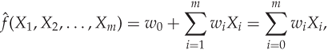

where we have fixed for the sake of brevity. Obviously, we need to choose the s to get the best possible prediction, but what do we mean by best possible?

We have already seen linear regression in action, as it was used to calculate the prediction error image for Farid's features in Section 7.3.2. The assumption was that each wavelet coefficient can be predicted using a function of coefficients , including adjacent coefficients, corresponding coefficients from adjacent wavelet components and corresponding coefficients from the other colour channels. Using the regression formula , denotes the image being tested, is the prediction image and the prediction error image.

The most common criterion for optimising the regression function is the method of least squares. It aims to minimise the squared error in (12.13). The calculation of the regression function can be described as a training phase. Although the term is not common in statistics, the principle is the same as in machine learning. The input to the regression algorithm is a sample of observations of the response variable , and corresponding observations of the predictor variable. The assumption is that depends on .

The linear predictor can be written in matrix form as

where the observation of the deterministic dummy variable is included in . Let be a column vector containing all the observed response variables, and let be an matrix containing the observed feature vectors as rows. The prediction errors on the training set can be calculated simultaneously using a matrix equation:

Thus the least-squares regression problem boils down to solving the optimisation problem

where

The minimum is the point where the derivative vanishes. Thus we need to solve

Hence, we get the solution given as

and the regression function (12.14) reads

This is the same formula we used for the linear predictor of Farid's features in Chapter 7.

12.3.2 Support Vector Regression

There is also a regression algorithm based on support vector machines. Schölkopf et al. (2000) even argue that support vector regression (SVR) is simpler than the classification algorithm, and that it is the natural first stage.

Note that the usual SVM algorithm results in a function , which may look like a regression function. The only problem with the standard SVM is that it is not optimised for regression, only for classification. When we formulate support vector regression, the function will have the same structure:

12.15

but the are tuned differently for classification and for regression.

A crucial property of SVM is that a relatively small number of support vectors are needed to describe the boundary hyperplanes. In order to carry this sparsity property over to regression, Vapnik (2000) introduced the -insensitive loss function:

12.16

In other words, prediction errors less than are accepted and ignored. The threshold is a free variable which can be optimised.

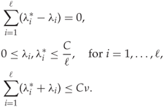
This leads to a new optimisation problem, which is similar to those we saw in Chapter 11:

The constants and are design parameters which are used to control the trade-off between minimising the slack variables and , the model complexity and the sensitivity threshold . The constraints simply say that the regression error should be bounded by plus some slack, and that the threshold and slack variables should be non-negative.

Using the standard techniques as with other SVM methods, we end up with a dual and simplified problem as follows:

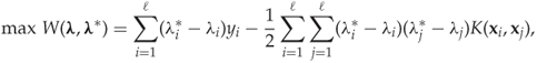
subject to

The solutions and are used to form the regression function

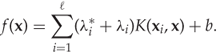
The most significant difference between this regression function and that from least-squares linear regression is of course that the kernel trick makes it non-linear. Hence much more complex dependencies can be modelled. There is support for SVM regression in libSVM.

12.4 Unsupervised Learning

The classifiers we have discussed so far employ supervised learning. That is, the input to the training algorithm is feature vectors with class labels, and the model is fitted to the known classes. In unsupervised learning, no labels are available to the training algorithm. When we use unsupervised learning for classification, the system will have to identify its own classes, or clusters, of objects which are similar. This is known as cluster analysis or clustering. Similarity often refers to Euclidean distance in feature space, but other similarity criteria could be used. This may be useful when no classification is known, and we want to see if there are interesting patterns to be recognised.

In general, supervised learning can be defined as learning in the presence of some error or reward function. The training algorithm receives feedback based on what the correct solution should be, and it adjusts the learning accordingly. In unsupervised learning, there is no such feedback, and the learning is a function of the data alone.

The practical difference between a ‘cluster’ as defined in cluster analysis and a ‘class’ as considered in classification is that a class is strictly defined whereas a cluster is more loosely defined. For instance, an image is either clean or a steganogram, and even though we cannot necessarily tell the difference by inspecting the image, the class is strictly determined by how the image was created. Clusters are defined only through the appearance of the object, and very often there will be no objective criteria by which to determine cluster membership. Otherwise clustering can be thought of, and is often used, as a method of classification.

We will only give one example of a statistical clustering algorithm. Readers who are interested in more hard-core learning algorithms, should look into the self-organising maps of Kohonen (1990).

12.4.1 -means Clustering

The -means clustering algorithm is a standard textbook example of clustering, and it is fairly easy to understand and implement. The symbol just denotes the number of clusters. A sample of objects, or feature vectors, is partitioned into clusters .

Each cluster is identified by its mean , and each object is assigned to the cluster corresponding to the closest mean, that is to minimise . The solution is found iteratively. When the mean is calculated, the cluster assignments have to change to keep the distances minimised, and when the cluster assignment changes, the means will suddenly be wrong and require updating. Thus we alternate between updating the means and the cluster assignments until the solution converges. To summarise, we get the following algorithm:

1. Choose random points for .

2. Form disjoint sets , so that if solves .

3. Update to be the sample mean of , i.e.

4. Repeat from Step 2 until the solution converges.

It can be shown that the solution always converges.

Code Example 12.3 : -means clustering in Python; the input X is an array with feature vectors as rows. The output is a pair , where is an integer array with element the index of the cluster containing and is a array where the th row is the mean of cluster

def kmeans(X,K=2,eps=0.1):
    (N,m) = X.shape
   M = np.random.randn(N,m)
   while True:
      L = [ np.sum( (X − M[[i],:])**2, axis=1 ) for i in xrange(K) ]
      A = np.vstack( L )
      C = np.argmin( A, axis=0 )
      L = [ np.mean( X[(C==i),:], axis=0 ) for i in xrange(K) ]
      M1 = np.vstack(M1)
      if np.sum((M−M1)**2) < eps: return (C,M1)
      else: M = M1

---

Code Example 12.3 shows how this can be done in Python. The example is designed to take advantage of efficient matrix algebra in numpy, at the expense of readability. The rows of the input are the feature vectors. Each row of is the mean of one cluster, and is initialised randomly. The matrix is , where . Then is calculated so that the th element is the index of the cluster containing , which corresponds to the row index of the maximal element in each column of . Finally, is calculated as the new sample mean of each cluster, to replace . If the squared Euclidean distance between and is smaller than a preset threshold we return, otherwise we reiterate.

Criticism and Drawbacks

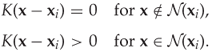
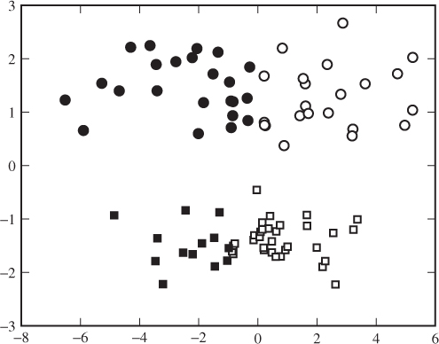
The -means algorithm is very intuitive and relatively fast. One may say it is too simplistic in that each cluster is defined only by its sample mean, without any notion of shape, density or volume. This can have some odd effects when the cluster shapes are far from spherical. Figure 12.3, for example, shows two elongated clusters, and human observers would probably focus on the gap between the upper and lower clusters. The -means algorithm, implicitly looking for spherical clusters, divides it into a lefts-hand and a right-hand cluster each containing about half each of the elongated clusters. Similar problems can occur if the clusters have very different sizes.

Figure 12.3 Elongated clusters with -means. Two sets, indicated by squares and circles, were generated using a Gaussian distribution with different variances and means. The colours, black and white, indicate the clustering found by -means for

Another question concerns the distance function, which is somewhat arbitrary. There is no objective reason to choose any one distance function over another. Euclidean distance is common, because it is the most well-known distance measure. Other distance functions may give very different solutions. For example, we can apply the kernel trick, and calculate the distance as

12.17

for some kernel function .

12.5 Summary

The fundamental classification problem on which we focused until the start of this chapter forms part of a wider discipline of pattern recognition. The problem has been studied in statistics since long before computerised learning became possible. Statistical methods, such as Bayesian classifiers in this chapter and Fisher linear discriminants in the previous one, tend to be faster than more modern algorithms like SVM.

We have seen examples of the wider area of pattern recognition, in unsupervised learning and in regression. Regression is known from applications in quantitative steganalysis, and unsupervised learning was used as an auxiliary function as part of the one-class steganalyser with multiple hyperspheres of Lyu and Farid (2004) (see Section 11.5.3). Still, we have just scratched the surface.