Chapter 14

The Steganalysis Problem

So far, we have defined steganalysis as the eavesdropper's problem, deciding whether or not a given information object contains covert information in addition to the overt information. In reality, the eavesdropper's problem is not so homogeneous. Different scenarios may require different types of steganalysis, and sometimes the eavesdropper needs more information about the covert message.

Generally, the difficulty of steganalysis decreases with the size of the covert message. An important question from the steganographer's point of view is ‘how much data can be embedded and still remain undetectable?’ This maximum quantity of undetectable information may be called the steganographic capacity. The concept of undetectable is a fuzzy concept, giving rise to a number of proposed security criteria.

In this chapter, we will discuss various use cases and how they call for different properties in steganalysers. We will also see how composite steganalytic systems can be designed, using multiple constituent steganalysers.

14.1 Different Use Cases

14.1.1 Who are Alice and Bob?

In the original phrasing of the problem, Alice and Bob are prisoners who want to use steganography to coordinate escape plans under the nose of Wendy. Already arrested, Alice and Bob are not necessarily assumed to be innocent. It is quite possible that Wendy does not need very strong evidence to withdraw their privilege by closing the communication line between Alice and Bob, and in any case she can dedicate special resources to the monitoring of their particular communication line. We will continue to refer to this scenario as the prisoners' problem.

Other user scenarios may be more or less different from the textbook scenario. Let us first consider a fairly similar one. Alice and Bob are still individuals, transmitting steganograms in a one-to-one conversation, but they are free citizens and not subject to any special legal limitations. They could be involved in organised crime, or they could be intelligence agents of a foreign power. In this case Wendy will need much stronger evidence in order to punish or restrain Alice and Bob; she must prove, beyond any reasonable doubt, that Alice and Bob are breaking the law. Furthermore, Alice and Bob may not receive any special attention from Wendy, as she must split her resources between a number of potential suspects. We will refer to this scenario as one-to-one steganography.

A popular, alleged scenario is Alice using steganography in a kind of broadcast dead-drop. Dead-drops traditionally refer to hiding places in public locations, where one agent could hide a message to be picked up by another at a later stage. In steganography, we imagine dead-drops on public Internet sites, where innocent-looking images can be posted, conveying secret messages to anyone who knows the secret key. Clearly, the intended receiver may be an individual, Bob (as before), or a large network of fellow conspirators. If the steganogram is posted on a site like eBay or Facebook, a lot of innocent and unknowing users are likely to see the image. Even when Alice is suspected of a conspiracy, Bob may not become more suspicious than a myriad other users downloading the same image. We call this scenario dead-drop steganography.

In all the scenarios mentioned so far, the message may be long or short. Alice and Bob may need to exchange maps, floor plans, and images, requiring several images at full capacity to hide the entire message. It is also possible that the message is very short, like ‘go tomorrow 8pm’, if the context is already known and shared by Alice and Bob. As we have seen, very short messages are almost impossible to detect, even from the most pedestrian stego-systems, while long messages are easily detectable with medieval steganalysers. We introduce a fourth user scenario that we call storage steganography, which focuses purely on very long messages. It arises from claims in the literature that paedophiles are using steganography to disguise their imagery. It may be useful for Alice to use steganography to hide the true nature of her data on her own system, even without any plans to communicate the steganograms to Bob. Thus, in the event of a police raid, it will hopefully be impossible for any raiders to identify suspicious material.

Most of the literature focuses on what we can call one-off steganography, where Wendy intercepts one steganogram and attempts to determine if it contains a message. In practice, this may not be the most plausible scenario. In an organised conspiracy, the members are likely to communicate regularly over a long period of time. In storage steganography, many steganograms will be needed to fit all the data that Alice wants to hide. Ker (2006) introduced the concept of batch steganography to cover this situation. Alice spreads the secret data over a batch of data objects, and Wendy faces a stream of potential steganograms. When she observes a large sample of steganograms, Wendy may have a better probability of getting statistically significant evidence of steganography.

The last question to consider with respect to Alice's viewpoint is message length, and we know that short messages are harder to detect than long ones. It goes without saying that sufficiently short messages are undetectable. Storage steganography would presumably require the embedding of many mega bytes, quite possibly giga bytes, to be useful. The same may be the case for organised crime and terrorist networks if detailed plans, surveillance photos, and maps need to be exchanged via steganography. For comparison, a 512 × 512 image can store 32 Kb of data using LSB embedding. The capacity for JPEG varies depending on the image texture and compression level, but about 3–4 kb is common for 512 × 512 images. Thus many images might be needed for steganograms in the above applications, and testing the steganalysis algorithms at 50–100% of capacity may be appropriate.

Operational communications within a subversive team, whether it belongs to secret services or the mob, need not require long messages. It might be a date and a time, say 10 characters or at most 21 bits in an optimised representation. An address is also possible, still 20–30 characters or less. Useful steganographic messages could therefore fit within 0.1%

of LSB capacity for pixmap images. Yet, in the steganalysis literature, messages less than 5% of capacity are rarely considered. Any message length is plausible, from a few bytes to as much as the cover image can take.

14.1.2 Wendy's Role

In the prisoners' problem, the very use of steganography is illegal. Furthermore, the prison environment may allow Wendy to impose punishment and withdraw privileges without solid proof. Just suspecting that it takes place may be sufficient for Wendy to block further communication. That is rarely the case in other scenarios. If Wendy is an intelligence agent, and Alice and Bob use steganography to hide a conspiracy, Wendy will usually have to identify the exact conspiracy in order to stop it, and solid proof is required to prosecute.

Very often, basic steganalysis will only be a first step, identifying images which require further scrutiny. Once plausible steganograms have been identified, other investigation techniques may be employed to gather evidence and intelligence. Extended steganalysis and image forensics may be used to gather information about the steganograms. Equally important, supporting evidence and intelligence from other sources may be used.

Even considering just the basic steganalyser, different use cases will lead to very different requirements. We will primarily look at the implications for the desired error probabilities and , but also some specialised areas of steganalysis.

Basic Steganalysis

The background for selecting the trade-off between and is an assessment of risk. We recall the Bayes risk, which we defined as

14.1

where c_x is the cost of a classification error and is the (a priori) probability that steganography is being used. We have assumed zero gain from correct classifications, because only the ‘net’ quantity is relevant for the analysis. The risk is the expected cost Wendy faces as a result of an imperfect steganalyser.

Most importantly, we must note that the risk depends on the probability of Alice using steganography. Hence, the lower is, the higher is the risk associated with false positives, and it will pay for Wendy to choose a steganalyser with higher and lower . To make an optimal choice, she needs to have some idea of what is.

In the prisoners' problem, one might assume that is large, possibly of the order of 10⁻¹, and we can probably get a long way with state-of-the-art steganalysers with about 5–10% false positives and . Storage steganography may have an even higher prior stego probability, as Wendy is unlikely to search Alice's storage without just cause and reason for suspicion.

A web crawler deployed to search the Web for applications of dead-drop steganography is quite another kettle of fish. Most web users do not know what steganography is, let alone use it. Even a steganography user will probably use it only on a fraction of the material posted. Being optimistic, maybe one in a hundred thousand images is a steganogram, i.e. . Suppose Wendy uses a very good steganalyser with and . In a sample of a hundred thousand images, she would then expect to find approximately a thousand false positives and one genuine steganogram.

Developing and testing classifiers with low error probabilities is very hard, because it requires an enormous test set. As we discussed in Chapter 3, 4000 images gives us a standard error of roughly 0.0055. In order to halve the standard error, we need four times as many test images. A common rule of thumb in error control coding, is to simulate until 100 error events. Applying this rule as a guideline, we would need about ten million test images to evaluate a steganalyser with an FP rate around .

One could argue that a steganalyser with a high false positive rate would be useful as a first stage of analysis, where the alleged steganograms are subject to a more rigorous but slower and more costly investigation. However, little is found in the literature on how to perform a second stage of steganalysis reliably. The first-stage steganalyser also needs to be accurate enough to give a manageable number of false positives. Wendy has to be able to afford the second-stage investigation of all the false positives. Even that may be hard for a web-crawling state-of-the-art steganalyser. The design of an effective steganalysis system to monitor broadcast channels remains an unsolved problem.

14.1.3 Pooled Steganalysis

Conventional steganalysis tests individual media objects independently. It is the individual file that is the target, rather than Alice as the source of files. Ker (2006) introduced the concept of batch steganography, where Alice spreads the secret data across multiple (a batch of) media objects. Wendy, in this scenario, would be faced with a stream of potential steganograms. It is not necessarily interesting to pin point exactly which objects contain secret data. Very often the main question is whether Alice uses steganography. Thus Wendy's objective should be to ascertain if at least one of the files is a steganogram. Traditional steganalysis does not exploit the information we could have by considering the full stream of media objects together.

A natural solution to this problem is called pooled steganalysis, where each image in the stream is subject to the same steganalyser, and the output is subject to joint statistical analysis to decide whether the stream as a whole is likely to contain covert information. Ker demonstrated that pooled steganalysis can do significantly better than the naïve application of the constituent algorithm. In particular, he showed that under certain assumptions, when the total message size n increases, the number of covers has to grow as n² to keep the steganalyst's success rate constant. This result has subsequently become known as the square-root law of steganography, and it has been proved under various cover models. It has also been verified experimentally.

Ker has analysed pooled steganalysis in detail under various assumptions, see for instance Ker (2007a). The square-root law was formulated by Ker (2007b) and verified experimentally by Ker et al. (2008). Notably, Ker (2006) showed that Alice's optimal strategy is not necessarily to spread the message across all covers. In some cases it is better to cluster it into one or a few covers.

The square-root law stems from the fact that the standard deviation of a statistic based on an accumulation of N observations grows as . We have seen this with the standard error in Section 3.2 and in the hypothesis test of Section 10.5.2. The proofs that the cover length N has to grow exactly as the square of the message length n are complicated and tedious, but it is quite easy to see that N has to grow faster than linearly in n. If we let N and n grow, while keeping a constant ratio n/N, then Wendy gets a larger statistical sample from the same distribution, and more reliable inference is possible.

In principle, batch steganography refers to one communications stream being split across multiple steganograms sent from Alice to Bob. The analysis may apply to other scenarios as well. If Wendy investigates Alice, and is interested in knowing whether she is using steganography to communicate with at least one of her contacts Bob, Ben or Bill (etc.), pooled steganalysis of everything transmitted by Alice can be useful. According to the square-root law, Alice would need to generate rapidly increasing amounts of innocent data in order to maintain a fixed rate of secret communications, which should make Wendy's task easy over time.

Finally, there is reason to think that the square-root law may tell us something about the importance of image size in the unpooled scenario; that doubling the message length should require a quadrupling of the image size. As far as we know, such a result has neither been proved analytically nor demonstrated empirically, but the argument about the variance of features going as should apply for most features also when N is the number of coefficients or pixels. If this is true, relative message length as a fraction of image size is not a relevant statistic.

14.1.4 Quantitative Steganalysis

Quantitative steganalysis aims to estimate the length of the hidden message. Both the approaches and the motivations vary. Where simple steganalysis is a classification problem, quantitative steganalysis is an estimation problem. Alice has embedded a message of q bits, where q may or may not be zero. We want to estimate q. Knowledge of q may allow Wendy to assess the seriousness of Alice and Bob's activities, and can thereby give useful intelligence.

We can formulate quantitative steganalysis as a regression problem, and as discussed in Section 12.3, both statistical and learning algorithms exist to solve it. Any feature vector which can be used with a learning classifier for basic steganalysis can in principle be reapplied with a regression model for quantitative steganalysis.

Quantitative steganalysis is not always an end in its own right. Sometimes we want to develop a statistical model to identify good features for classification, and we find an estimator for q as a natural component in the model. Quite commonly is abused as a measure of confidence; the larger is the more confidently we conclude that the image contains a hidden message. Even though this idea can be justified qualitatively, there is no clear quantitative relationship. We cannot use directly to quantify the level of confidence or significance.

Applying a quantitative steganalyser to the basic steganalysis problem is possible, but it is not as straightforward as one might think. In fact, it is very similar to using any other feature for classification. We have to select a threshold τ and assume a steganogram for and a clean image for . The threshold must be selected so that the error rates and are acceptable. Optimising the threshold τ is exactly what a classification algorithm aims to do.

Sometimes, one may want to assess without explicitly selecting τ, merely making a subjective distinction of whether or . This can give an implicit and subjective assessment of the level of confidence. A numeric measure of confidence is very useful, but there are better alternatives which allow an objective assessment of confidence. A good candidate is a Bayesian estimate for the posterior probability . The p-value from a hypothesis test also offers some objectivity. In libSVM, for example, such probability estimates can be obtained using the -b 1 option.

14.2 Images and Training Sets

As important for steganalysis as the selection of features, is the choice of training set. In the last few years, steganalysts have become increasingly aware of the so-called cover-source mismatch problem. A steganalyser trained on images based on one cover source may not perform nearly as well when presented with images from a different source.

A closely related question is the one asked by Alice. What cover source will make the steganograms most difficult to detect? Wendy should try to use a cover source resembling that used by Alice. Without knowing exactly what Alice knows, it is useful to know how to identify covers which make detection hard. In this chapter we will consider some properties of covers and cover sources that affect detection probability.

14.2.1 Choosing the Cover Source

It is straight forward to compare given cover sources, and a number of authors have indeed compared classes of covers, focusing on different characteristics. For each class of cover images, we can train and test a steganalyser; and compare the performance for the same feature vector and classifier algorithm but for different cover sources. If the steganalyser has poor performance for a given source, that means this particular source is well suited from Alice's point of view.

This only lets us compare sources. Searching for the ideal cover source remains hard because of the vast number of possibilities. Furthermore, the analysis cannot be expected to be consistent across different steganalysers, and we would therefore have to repeat the comparison for different steganalysers, in much the same way as a comparison of steganalysers must be repeated for different cover sources.

Image Sources

From capturing to its use in steganography or steganalysis, an image undergoes a number of processes. First is the physical capturing device, with its lenses and image sensor. Second, the image may be subject to in-camera image processing and compression, and finally, it may be subject to one or more rounds of post-processing and recompression. Post-processing may include colour, brightness and contrast correction or other tools for quality enhancement. It may also include downsampling, cropping or recompression to adapt it for publication in particular fora.

The motive and texture of the image can affect the results. Light conditions will have obvious and significant effects on image quality, and there may also be differences between outdoor/indoor, flash, lamp light and daylight, and between people, landscapes and animals.

Many of the differences between different image sources can be explained in terms of noise. Many of the known feature vectors are designed to detect the high-frequency noise caused by embedding, but obviously the steganalyser cannot distinguish between embedding distortion and naturally occurring noise, and clean images have widely varying levels of natural noise. Highly compressed images, where the high-frequency noise has been lost in compression, will offer less camouflage to hide the embedded message. Contrarily, images with a lot of texture will offer good camouflage for a hidden message. Different capturing devices may cause different levels of high-frequency noise depending on their quality.

Authors in steganalysis typically draw their images from published collections such as UCID (Schaefer and Stich, 2004), Corel, Greenspun (2011) or NRCS (Service, 2009). This will usually mean high-quality images, but we usually do not know if they have been subject to post-processing. Some also use own-captured images, and again, as readers we do not know the characteristics of these images. A number of image databases have been published specifically for research in steganography and watermarking, and these tend to be well-documented. Most notable are the two 10 000 image databases used for the BOWS (Ecrypt Network of Excellence, 2008) and BOSS (Filler et al., 2011b) contests, but also one by Petitcolas (2009).

In an extensive performance analysis of steganalysers based on Farid-72, FRI-23 and BSM-xx, Kharrazi et al. (2006b) used a large number of images acquired with a web crawler. This gave them a more diverse set of images than previous evaluations. They separated the images into high, medium and low compression quality, and trained and tested the steganalysers on each class separately. Unsurprisingly, the low-quality images gave the most detectable steganograms.

The capturing device is known to have a significant effect on the detectability. Wahab (2011) has tested this for Farid-72 and FRI-23, where the steganalyser was trained and tested on images from different capturing devices. It was found that FRI-23 was remarkably robust against changes in image source, whereas Farid-72 was significantly less accurate when it was trained and tested on different image sources.

The question of capturing device can be very specific. Goljan et al. (2006) showed that detection performance may improve by training the classifier on images from the exact same camera, compared with training on images from another camera of the same make and model. This may be surprising at first glance, but should not be. Microscopic devices, such as the image sensor, will invariably have defects which are individual to each unit produced. Adequate performance is achieved through redundancy, so that a certain number of defects can be tolerated. Defects in the image sensor cause a noise pattern which is visually imperceptible, but which may be picked up statistically by a steganalyser or similar system.

Another important image characteristic, which has been analysed by Liu et al. (2008), is that of texture. They considered the diagonal sub-band of the Haar wavelet decomposition in order to quantify the texturing. The distribution of coefficient values is modelled using a generalised Gaussian distribution (GGD), which is defined as

where for z > 0 is the Gamma function. The σ parameter is just the standard deviation, but the so-called shape parameter β of the diagonal Haar band is a measure of the texture complexity of the pixmap image. Liu et al. showed that steganalysers with an accuracy of more than 90% for images with little texture (β < 0.4) could be as bad as < 55%

for highly textured images with β > 1.

Choosing Cover for Embedding

The selection of a good cover is part of Alice's strategy and has long been recognised as an important problem even if it remains only partially solved. Lately, some authors have started to devise methods to filter the cover source to select individual images that are particularly well suited.

Filter methods may be general or message-specific. A general method would determine whether a given cover is suitable for messages of a particular length, whereas a message-specific method would check if a given steganogram, with a specific message embedded, is likely to go undetected.

In one of the earlier works on the topic, Kharrazi et al. (2006a) analysed a number of heuristics for cover selection. General methods can be as simple as counting the number of changeable coefficients. Embedding in a cover with many changeable coefficients means that the relative number of changes will be small. For LSB embedding this obviously corresponds to image size, but for JPEG embedding, zero coefficients are typically ignored, so highly textured or high-quality images will tend to give less detectable steganograms.

Sajedi and Jamzad (2009) proposed a general filter method which is considerably more expensive in computational terms. They estimated embedding capacity by trial and error, by embedding different length messages and checking the detectability in common steganalysers. The capacity can then be defined as the length of the longest undetectable message. The images and their capacity can then be stored in a database. When a given message is going to be sent, the cover is selected randomly from those images with sufficient capacity.

14.2.2 The Training Scenario

By now, it should be clear that all universal steganalysers must be very carefully trained for the particular application. A steganalyser is designed to detect artifacts in the images. It will pick up on any artifact which statistically separates the classes in the training set, whether or not those artifacts are typical for the two classes in the global population. These artifacts may or may not be typical for steganography, and they are unlikely to be unique to steganography. For instance, a steganalyser which is sensitive to the high-frequency noise caused by embedding will make many false positives when it is presented with clean images with a higher level of naturally occurring noise.

The design of the training scenario is part of the steganalyst strategy. Obviously, it requires an understanding of Alice's choice of images as discussed in the previous section. Furthermore, the cover source favoured by Alice the steganographer is not necessarily related to the source of clean images transmitted by the innocent Alice. Hence there are potentially two different image distributions that must be understood. This issue may be too hard to tackle though; all known authors use the same source for clean images and cover images. But we will look into a couple of other concerns that we need to be aware of regarding the preparation of images.

Image Pre-processing

Many of the common features in steganalysis may depend on irrelevant attributes such as the image size. It is therefore customary to pre-process the images to make them as comparable as possible.

The most obvious example of size-dependent features are those derived from the histogram. Very often the absolute histogram is used, and a larger image will have larger histogram values. This can be rectified by using the relative histogram, which is the absolute histogram divided by the total number of coefficients. Other features may depend on size in a less obvious way.

The most common approach to dealing with this problem is to crop all images to one pre-defined size. Scaling has been used by some authors, but is generally considered to be more likely to introduce its own artifacts than cropping is. This approach works well for training and testing of the steganalyser, but it does not tell us how to deal with off-size images under suspicion. We can crop the intercepted image prior to classification, but then we discard information, and what happens if the secret message is hidden close to the edges and we crop away all of it? We could divide the image into several, possibly overlapping, regions and steganalyse each of them separately, but then the problem would essentially become one of detecting batch steganography and we should design the steganalyser accordingly.

For a production system, all the features should be normalised to be independent of the image size. This is not necessarily difficult, but every individual feature must be assessed and normalised as appropriate, and few authors have considered it to date.

Double Compression

Of all the irrelevant artifacts which can fool a steganalyser, double compression is probably the strongest, and certainly the most well-known one. It is the result of a bug in the common implementations of algorithms like F5 and JSteg. When the software is given a JPEG image as input, this is decompressed using common library functions, and the quantisation tables discarded. The image is then recompressed using default quantisation tables, possibly with a user-defined quality factor, and the embedding is performed during recompression.

The result is that the steganograms have been compressed twice, typically with different quality factors. This double compression leaves artifacts which are very easy to detect. Early works in steganalysis would train the steganalyser to distinguish between single-compressed natural images and double-compressed steganograms. What are we then detecting? Double compression or steganographic embedding?

This training scenario will fail both if Alice has a different implementation of F5, or she uses uncompressed images as input; and it will fail if doubly compressed but clean images occur on the channel. The first case will lead to a high false negative probability, and the second to many false positives. The problem was first pointed out by Kharrazi et al. (2006b), who compared a steganalyser with a training set where both natural images and steganograms were double compressed. This training scenario gave much lower accuracies than the traditional training scenario. Later, Wahab (2011) made similar tests with a training set where both the natural images and steganograms were compressed once only, and found similar results.

Double compression is not uncommon. Images captured and stored with high-quality compression will often have to be recompressed at a lower quality to allow distribution on web pages or in email. It is also common that images are converted between image formats, including uncompressed formats, as they are shared between friends, and this may also lead to recompression at a higher quality factor than previous compressions, as the user will not know how the image previously compressed. Thus it is clear that evidence of double compression is no good indication of steganography, and the steganalyser has to be able to distinguish between steganograms and clean images whether they are singly or doubly compressed.

It is obvious that we need to train the steganalyser on every embedding algorithm we expect steganographers to use. The double-compression problem tells us that we may have to train it for every conceivable implementation of the algorithm as well. In addition to the well-studied double-compression bug, there may be other implementation artifacts which have not yet been discovered.

Embedding and Message Length

Each steganogram in the training set has to be embedded with some specific message using a specific algorithm. We usually train the steganalyser for a specific embedding algorithm, and the significance of this choice should be obvious.

The choice of message can also affect the steganalysis. The visual steganalysis discussed in Section 5.1 showed us how different types of messages leave different artifacts in the LSB plane. In general, higher-order features studying relationships between different bits or pixels will respond very differently to random message data and more structured data such as text. The most common choice, especially in recent years, is to use random messages for training and testing, and there are many good reasons for this.

In real life, random-looking messages are the result of compressing and/or encrypting the data. Both compression and encryption are designed to produce random-looking data. Compression because it removes any redundancy which would cause the statistical structure, and encryption because random-looking data gives the least information for the eavesdropper. Compression will reduce the number of embedding changes and thereby make the embedding less detectable. Alice may also want to encrypt the message to protect the contents even if the existence were to be detected. Hence, random-looking messages are very plausible.

If Alice were to go for non-random-looking data she should, as we saw in the discussion of Bayes' classifiers, aim for a probability distribution resembling that of the cover image. The easiest way to achieve this is to use a random-looking message and embed it in random-looking data. Otherwise, it is very hard to find a message source and a cover source with matching distributions. Although some may exist, there are no known examples where a random-looking message is easier to detect than a non-random one. Again, Alice has the best chance by using random-looking messages.

The next question for the training phase is what message lengths to consider. Commonly, new classifiers are trained and tested for a number of message lengths, specified as a fraction of capacity, typically ranging from 5% to 100%. This has a number of problems. Although capacity is well-defined for LSB embedding, as one bit per pixel, it is ill-defined for many other algorithms. In JPEG steganalysis, one often specifies the message length in bits per non-zero coefficients (bpc). This overestimates capacity for JSteg and Outguess 0.1, which cannot use coefficients equal to one either. In F4 and F5 the capacity in bits will depend on the contents of the message, because re-embedding occurs as the result of specific bit values.

All of these measures relate, even if loosely, to the physical capacity of the cover image, and are unrelated to the detectability. The square-root law indicates that even if 5% of messages are detectable for a given size of cover image, they may not be detectable if sufficiently small images are used. Detectability depends both on cover size and message length, not just on the ratio between them.

In this book, we have tended to use a constant message length in bytes or in bits for all images. For LSB embedding with a fixed image size in the spatial domain, this is of course equivalent to fixing a relative message length. For JPEG, in contrast, it will be different because the capacity will depend on image texture as well as image size. The choice to use constant length in bits is motivated by the practical requirements seen by Alice. She will have a specific message which she needs to send to Bob. The message length is determined only by Alice's usage scenario and not at all by the cover image. This approach, however, ignores cover selection. If Alice's uses cover selection, many of the cover's in the training and test sets would be ineligible as covers for the particular message length.

Capacity and Message Length for F5

When designing a training scenario, it is useful to consider what parameters the stego-system has been designed for. This is especially true when steganalysis is used to evaluate the stego-system. Far too often, stego-systems are evaluated and criticised under conditions they were never intended for. Take F5 as an example. Using F5 at maximum capacity would mean that every non-zero coefficient is needed for the payload, and matrix coding cannot be used to reduce the number of embedding changes. Thus F5 degenerates to F4.

Briffa et al. (2009b) report some tests of the capacity of F5. The matrix code is an [2^k − 1, 2^k − 1 − k, 3] Hamming code, which means that k bits are embedded using 2^k − 1 changeable coefficients. According to Briffa et al., embedding at k = 1 typically hides 1.4 message bits per modified coefficients. At k = 4 we almost always get two message bits per change, typically 2.1–2.5. At k = 7, which is the maximum k in Westfeld's implementation, we can typically embed 3.5–4 bits per change.

In order to reduce the distortion by 50% compared to F4, the minimum value is k = 5, which gives a code rate of between 1/6 and 1/7. Because of the re-embeddings where zeros are created, the embedding rate in bpc will be considerably lower than the code rate. At k = 7 we have a code rate of 0.055, while the empirical embedding capacity according to Briffa et al. is about 0.008 bpc on average. In other words, in order to get a significant benefit from matrix coding, F5 should only be used at embedding rates of a few percent of the number of non-zero coefficients. In the literature we often see 5% as the low end of the range of message lengths considered, but for F5 it should rather have been the high end.

The Size of the Training Set

The required size of the training set is probably the most obvious question regarding the training scenario. We have left it till the end because it is also the hardest. Miche et al. (2007) did suggest an approach to determine a good training set size for a given cover source. Starting with a total training set of 8 000 images, they ran a Monte Carlo simulation repeatedly, selecting a smaller training set randomly. The classifier was trained on the smaller set and tested on a separate set of 5000 images. Testing different training set sizes, from 200 to 4000, they found that the accuracy converged and little was gained from using more than 2000 images for testing.

There is no reason to expect that the result of Miche et al. generalises. The more diverse the image base is, the larger the training set will have to be in order to be representative. It is, however, possible to use their methodology to determine a sufficient training set for other scenarios. Where one has access to a large image base, this may be a useful exercise.

14.2.3 The Steganalytic Game

The steganography/steganalysis problem can be phrased as a two-player game, where Alice and Wendy are the players. Alice transmits one or more files, with or without steganographic contents. Wendy attempts to guess whether there is a steganographic content or not. If Wendy guesses correctly she wins, otherwise she loses. When the game is complete, each player receives a payoff, which is usually normalised for a zero-sum game where the winner receives an amount x and the loser receives − x. The payoff is essentially the same quantity as the costs and which we used to define risk.

Considering practical applications of steganalysis, the game is exceedingly complex. Both Alice and Wendy have a number of strategic choices to make. Alice can not only choose whether or not to use steganography, she can also choose

• stego-algorithm,
• cover image,
• pre-processing of the cover image,
• message length,
• and possibly transmission channel.

Similarly, Wendy can choose

• feature vector,
• classification algorithm,
• training set(s), including

• decision threshold (trade-off between and ).

Clearly, the probability of success of Wendy's strategy will depend on Alice's strategy and vice versa. Wendy's optimal strategy may no longer be optimal if Alice changes hers.

Game theory is a well-established field within economics and mathematics, and has found applications in many other areas, including engineering problems such as power control in cellular networks. In theory, it allows us to calculate optimal strategies for the two players analytically. However, the strategy options we have listed above are far too many to allow an analytic solution. Instead, the formulated game highlights the complexity of the problem.

A key characteristic of any game is who moves first. Does one player know the strategy of the other player before she makes her own move? If Alice knows Wendy's strategy, she would of course test tentative steganograms against Wendy's strategy and reject any which are detectable. This may be the case if Wendy is part of a large-scale public operation, as it is then difficult to keep her methods secret. Similarly, if Wendy knows Alice's strategy, she would tune her steganalyser to that strategy. Although it may be unlikely that Wendy knows Alice's strategy in full, she might have partial information from other investigations, such as knowing that Alice has a particular piece of stego software installed.

Looking at Wendy's problem in general, it is reasonable to expect that Wendy and Alice move simultaneously and have to choose a strategy with no knowledge of the other player.

14.3 Composite Classifier Systems

A simple steganalyser as discussed so far consists of a single instance of the classifier algorithm. It is trained once, resulting in one model instance, which is later used for classification. The simple steganalyser is tuned for a particular training set, and may have poor performance on images which are very different from the training set. Very often, it is useful to combine several steganalysers or classifiers into a more complex steganalysis system.

We will start with a discussion of fusion, where multiple constituent classifiers are designed to solve the same classification problem, and then combined into a single classifier which will hopefully be more accurate. Afterwards, we will look at other composite steganalysis systems, where the classification problem is split between different classifiers, both steganalysers and other classifiers.

14.3.1 Fusion

Fusion refers to several standard techniques in machine learning. Very often, good classification results can be obtained by combining a number of mediocre classifiers. The simplest form of fusion is feature-level fusion, where multiple feature vectors are fused together to form a new, higher-dimensional feature vector. The fused feature vector can be used exactly like the constituent feature vectors, and we discussed examples of this in Chapter 13 without thinking of it as a new technique. The main drawback of feature-level fusion is the curse of dimensionality, and it is often necessary to combine it with feature selection to get reasonable performance. Other than the increase in dimensionality there is no change to the classification problem, and we will typically use the same algorithms as we do in the unfused scenario.

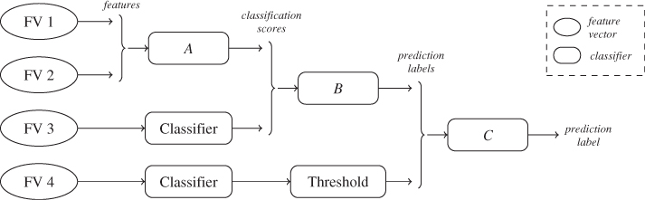
It is also possible to fuse classifiers based on the output of the constituent classifiers. Figure 14.1 shows how fusion operates at different layers with four different constituent feature vectors FV1–4. Classifier A uses feature-level fusion as discussed before; the two feature vectors FV1 and FV2 jointly form the input for A. Classifier B uses heuristic-level or measurement-level fusion, where the classification scores of the constituent classifiers form the input. Finally, classifiers can be fused at the classifier level or abstract level, as classifier C. Where heuristic-level classifiers use the soft information from the constituent classifiers, a classifier-level classifier uses the discrete label predictions after the classification scores have been thresholded.

Figure 14.1 The three types of fused classifiers: feature-level (A), heuristic-level (B), and classifier-level (C)

Both heuristic-level and classifier-level fusion avoid the curse of dimensionality unless a truly impressive number of constituent classifiers is used, but there is also another advantage over feature-level fusion. When we augment an existing classifier with new features, feature-level fusion requires complete retraining (and possibly new feature selection), which can be expensive when large data sets are involved. When fusion is based on classifier output, we can simply train a new classifier using the new features and add it to the fused classifier without retraining the other constituent classifiers. Since the fused classifier works with fewer features, and often uses a simpler algorithm, it will be much faster to train.

There is a wide range of possible algorithms which may be suitable for the fused classifier. One possibility is to view the input classification scores like any other feature vector and use a generic algorithm like SVM, FLD or neural networks, just as in the unfused case. Thus no new theory is necessary to handle fusion. This approach is also simple because we do not need any semantic interpretation of the classification scores. The constituent classifiers do not even have to produce scores on the same scale; instead we trust the learning algorithm to figure it out. More commonly, perhaps, the heuristic-level fused classification problem is solved by much simpler algorithms, exploiting the fact that we usually have much more knowledge about the probability distribution of the classifier output than we have for the original features.

Many classifiers, including Bayesian ones, output a posteriori probabilities that a given image I belongs to class i, and it is usually possible to get such probability estimates by statistical analysis of the classifier output. Given probability estimates for each class, it is possible to base the fused classifier on analysis instead of machine learning. In the context of steganalysis, Kharrazi et al. (2006c) tested two such fusion algorithms, namely the mean and maximum rules which we discuss below. A more extensive overview of fusion can be found in Kittler et al. (1998).

Let denote the posterior probability estimate from classifier j. The mean rule considers all the classifiers by taking the average of all the probability estimates; this leads to a new probability estimate

14.2

and the predicted class is the one maximising . The mean rule is based on the common and general idea of averaging multiple measurements to get one estimate with lower variance, making it a natural and reasonable classification rule.

The maximum rule will trust the classifier which gives the most confident decision, i.e. the one with the highest posterior probability for any class. The predicted class is given as

The maximum rule is used in the one-against-one and one-against-all schemes used to design multi-class classifiers from binary ones. It is a logical criterion when some of the classifiers may be irrelevant for the object at hand, for instance because the object is drawn from a class which was not present in the training set. Using the mean rule, all of the irrelevant classifiers would add noise to the fused probability estimate, which is worth avoiding. By a similar argument, one could also expect that the maximum rule will be preferable when fusing classifiers trained on different cover sources.

In classifier-level fusion, the input is a vector of discrete variables where each is a predicted class label rather than the usual floating point feature vectors. Therefore standard classification algorithms are rarely used. The most common algorithm is majority-vote, where the fused classifier returns the class label predicted by the largest number of constituent classifiers. Compared to heuristic-level fusion, classifier-level fusion has the advantage of using the constituent classifiers purely as black boxes, and thus we can use classifier implementations which do not provide ready access to soft information. On the contrary, if soft information is available, classifier-level fusion will discard information which could be very useful for the solution.

14.3.2 A Multi-layer Classifier for JPEG

Multi-layer steganalysis can be very different from fusion. Fusion subjects the suspect image to every constituent classifier in parallel and combines the output. In multi-layer steganalysis, the classifiers are organised sequentially and the outcome of one constituent classifier decides which classifier will be used next.

A good example of a multi-layer steganalysis system is that of Pevný and Fridrich (2008) for JPEG steganalysis. They considered both the problem of single and double compression and the issue of varying quality factor in steganalysis. To illustrate the idea, we consider quality factors first. We know that the statistical properties of JPEG images are very different depending on the quality factor. The core idea is to use one classifier (or estimator) to estimate the quality factor, and then use a steganalyser which has been trained particularly for this quality factor only. Because the steganalyser is specialised for a limited class of cover images, it can be more accurate than a more general one.

The design of multi-layer classifiers is non-trivial, and may not always work. Obviously we introduce a risk of misclassification in the first stage, which would then result in an inappropriate classifier being used in the second stage. In order to succeed, the gain in accuracy from the specialised steganalyser must outweigh the risk of misclassification in the first stage. The quality factor is a good criterion for the first classifier, because the statistical artifacts are fairly well understood. It is probably easier to estimate the quality factor than it is to steganalyse.

Another problem which can be tackled by a multi-layer classifier is that of double and single compression of JPEG steganograms. Just as they distinguished between compression levels, Pevný and Fridrich (2008) proposed to resolve the double-compression problem by first using a classifier to distinguish between singly and doubly compressed images, and subsequently running a steganalyser specialised for doubly or singly compressed images as appropriate.

14.3.3 Benefits of Composite Classifiers

Heuristic-level fusion is most often described as a fusion of constituent classifiers using different feature vectors. Implicitly one may assume that all the classifiers are trained with the same training sets. However, the potential uses do not stop there.

Fusion is a way to reduce the complexity of the classifiers, by reducing either the number of features or the number of training vectors seen by each constituent classifier. This can speed up the training phase or improve the accuracy, or both. It can also make it possible to analyse part of the model, by studying the statistics of each constituent classifier. When we discussed the application of SPAM features for colour images, it was suggested to train one classifier per colour channel, and then use heuristic- or abstract-level fusion to combine the three. Thus, each classifier will see only one-third of the features, and this reduces the risk of the curse of dimensionality and may speed up training.

The multi-layer classifier described in the previous section uses constituent classifiers with the same feature vector but different training sets. Kharrazi et al. (2006c) proposed using the same idea with fusion, training different instances of the classifier against different embedding algorithms. When new stego-systems are discovered, a new constituent classifier can be trained for the new algorithm and added to the fused classifier. This is essentially the one-against-one scheme that we used to construct a multi-class SVM in Section 11.4, except that we do not necessarily distinguish between the different classes of steganograms. Thus, it may be sufficient to have one binary steganalyser per stego-system, comparing steganograms from one system against clean images, without any need for steganalysers comparing steganograms from two different stego-systems.

On a similar note, we could use constituent classifiers specialised for particular cover sources. The general problem we face in steganalysis is that the variability within the class of clean images is large compared to the difference between the steganograms and clean images. This is the case whether we compare feature vectors or classification heuristics. Multi-layer steganalysis is useful when we can isolate classes of cover images with a lower variance within the class. When the steganalyser is specialised by training on a narrower set of cover images it can achieve higher accuracy, and this can form the basis for a multi-layer steganalyser. There are many options which have not been reported in the literature.

14.4 Summary

The evolution of steganography and steganalysis is often described as a race between steganalysts and steganographers. Every new stego-system prompts the development of a new and better steganalysis algorithm to break it; and vice versa. This chapter illustrates that it is not that simple.

New algorithms have been tested under laboratory conditions, with one or a few cover sources, and the detection accuracies normally end up in the range of 70–90%. Even though some authors test many sets of parameters, the selection is still sparse within the universe of possible use cases. Very little is known about field conditions, and new methods are currently emerging to let Alice select particularly favourable cover images, making the steganalyst laboratory conditions increasingly irrelevant. Removing the focus from feature vectors and embedding algorithms, the race between Alice and Wendy could take on a whole new pace  …

The parameters in the recent BOSS contest (Bas et al. 2011) are typical for empirical discussions of steganalysis, and may serve as an illustration without any intended criticism of the BOSS project, which has resulted in a few very useful additions to the literature. The data set for the HUGO stego-system used steganograms at 40% of capacity, and the winner achieved 80.3% accuracy. From a theoretical point of view, this has led to the conclusion that HUGO is no longer undetectable. Yet two questions are left unanswered here, as for many other stego-systems and steganalysers:

Such questions should be asked more often.