This example dataset goes from January 31st 2017 to March 11th 2017. Despite being from the past, we can contrive a scenario in which we are pretending to be in that time frame and say that today's date is March 1^st, 2017. We therefore want to have an ML job analyze the data between January 31st and today, and then use ML to forecast that data ten days into the future.

We can then have the ML job analyze the rest of the data in the index (from March 1^st through March 11^th) and we can see how close the forecast tracked the actual dataset. Let's begin!

The first step is to create a Single Metric job that uses the Sum aggregation function on the #amount field with a Bucket span of 15m:

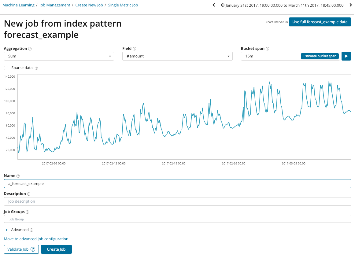
However, we don't want to analyze all of the data; we want to stop short on March 1^st. Therefore, in the top right, change the end date of the Kibana date picker to be March 1^st:

With that date modification made, you can name the job a_forecast_example and click the Create Job button:

Once the job has run, we can see the results preview in the UI:

To access the ability to forecast, we need to click the View Results button, which will take us to the Single Metric Viewer. In the Single Metric Viewer, we can see the overall dataset and can appreciate the shape and complexity of the way this data behaves; there are both daily and weekly periodic components, as well as a gradual positive slope/trend that causes the data to drift up over time:

Remember, despite the fact that we may only be interested in forecasting on this data, the ML job will still point out anomalies throughout the data's history, but we can simply ignore them.

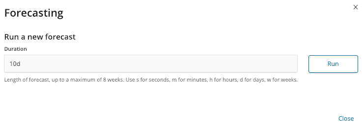
To invoke a forecast on this data, click the Forecast button and in the dialog box, enter a duration of 10 days (10d):

Clicking the Run button will invoke the forecast request, which will run in the background, but once finished will display the results of the forecast to extend over the time period of interest:

The shaded area around the forecast/predicted zone is the 95^th percentile confidence interval. In other words, ML has estimated that there is a 95% chance that the future values will be within this range (and likewise, only a 2.5% chance that the future values will be either above or below the confidence interval). The 95^th percentile range is currently a fixed value and is not yet settable by the user.

Now that we have the ability to create simple forecasts from the UI, let's explore the results of the forecast in more depth before moving to a more complicated example.