Introduction
This short chapter introduces the reader to the next step in WFMA (or perhaps a step beyond), and a step which will probably be part of the future for many forward-thinking readers. This to use the static models of a workflow map as produced by the Kmetz method covered in Chapters 3 and 4 to prepare a dynamic model of the workflow. This is more than simply a minor progression from a workflow map for reasons we will see below.
The concept of dynamic modeling is not new, and there are several classic studies in which the technique has been applied to produce very interesting results. Two of the best of these are articles published by Roger Hall on the decline and eventual failure of the old Saturday Evening Post magazine.1 In these studies, Hall, who had access to the records of the Board of Directors, was able to simulate the consequences of board decisions over time; what he found was that because the board and top management did not understand the interaction between several key business variables they controlled, their decisions ultimately led to outcomes which were exactly the opposite of what was intended. The magazine ultimately became financially unsustainable and failed after a successful period of publication that was claimed to have begun with Benjamin Franklin. Hall was able to model the management decisions and their unintended effects, and thereby explain how these produced the consequences that felled the magazine.
In recent years, companies have been applying dynamic modeling as a management tool to a greater extent than ever before. Among Scandinavian companies, according to some reports, nearly 30% of firms regularly use simulation tools as aids to strategy formulation and decision making2 Procter & Gamble, the global consumer goods company, uses simulation as one of four major types of “operations research” tools to support similar functions. This clearly is a growing category of business applications and in the right hands adds considerable economic value to those firms.
Unlike the WFMA methods we have been working with up to this point, dynamic modeling is a software-intensive undertaking, and is completely dependent on software support. Also unlike the mapping tools developed in this book, learning to use simulation software requires much more investment of time and energy. The objective of this chapter is not to turn the reader into a dynamic modeler, or to promote any particular software—it is to inform the reader of how WFMA enables taking the next step, the potential to use dynamic modeling to test ideas about how things might transpire in a virtual mode, and thus illustrate the potential of simulation. For most professional readers, application of such dynamic modeling will need to be relegated to staff specialists or consultants. In this regard, this chapter is a departure from the norms of my method, but I am convinced that the future will see several types of dynamic modeling become as widespread as static modeling is now. Indeed, some of the complexity of BPM and related software packages is because these are already including some elements of dynamic modeling. Ironically, I like that aspect of these packages, but I wish there were a clearer line between process mapping as I think of it and simulation through dynamic modeling.
What Is “Simulation?”
“Simulation” covers a very broad range of activities, including things like disaster-training exercises, fire drills, and the like. The kind of simulation we are concerned with in this chapter is the computer-based virtual modeling of a system, and in this case that model is restricted to measures and quantifiable variables and the relationships between them over time. It is a partial representation of a system—variables like employee motivation, innovation capabilities, and many other extremely important intangible properties of that system are either ignored or necessarily reduced to a limited approximation of the real thing.
Simulation has long been used in engineering and the sciences, in the form of models and scale representations of physical objects, whether atoms or bridges. Computer simulations like those we are discussing did not become feasible until roughly third-generation mainframe computers became available, in the 1960s and 1970s. One of the pioneers of business modeling is Jay W. Forrester, who published Industrial Dynamics in 1961, followed by a series of books on systems theory and “systems dynamics”; he is widely considered to be the father of systems dynamics as a field of study.3 His publication of World Dynamics came at the end of this fruitful decade of work, and at the same time created major concern about the future of the planet, being written in an era when the Club of Rome had also published Limits to Growth, which made many dire predictions.4
Much of what Forrester accomplished during this era and later years was to bring the importance of understanding systems into focus while at the same time illustrating the capability of computers to model them. More correctly, what the computers enabled was the testing of our “mental model” of a system, first through evaluation of our understanding of the components of the system and their relationships to each other, and then through the ability to use that model to simulate system outcomes and demonstrate parallels between the model and the real system.5 Obviously, this is highly consistent with my workflow mapping approach.
My personal involvement with dynamic modeling began with assisting several large defense contractors during the early and mid-1980s with construction and validation of dynamic models, based on my knowledge of the avionics maintenance workflow and system. One company in particular mounted a massive effort, involving over 30 people for a period of six months, to prepare and validate such a model. All of this was done writing original Fortran code and using modules of prepared simulation language programs.
The ability to create digital representations of systems in the early days of modeling required considerable skill in mathematics and computer programming, keeping much of this work in an esoteric realm of specialist knowledge and often making its results difficult to understand or believe. Since then, advances in programming and software development have made graphic interfaces for modelers available, such that the literal ability to draw a map of a workflow, subject to a few rules, is enough to model it—the software writes the equations and the code for you. This has revolutionalized accessibility to modeling, and several programs have been adopted so widely that user groups around the world have made them a de facto standard for systems modeling. Two of these programs are Stella, primarily a research tool, and iThink, used primarily for business modeling, both of which are published by isee systems (www.iseesystems.com). Fisher has published an excellent, non-technical and very readable training manual for new users.6
Creating and Using Dynamic Models
Map, then model
Successful dynamic modeling requires thorough understanding of the major variables and relationships between them in the workflow(s) being modeled. WFMA provides the static-model basis for development of a dynamic model. A validated map, as described in Chapters 3 and 4, is usually the best place to start simply because it is a valid map. This establishes a baseline for both initial construction of the model and for testing it to determine that we have translated the workflow map into a model correctly.
The need for “translation” arises because the symbols and terminology used in dynamic models are different from those we use in WFMA. Dynamic models consist of “stocks,” “flows,” and “rates,” and the WFMA workflow map we begin with must be converted into these variables in the dynamic model. Not surprisingly, the primary type of variable captured in a workflow map is termed a “flow” in dynamic modeling; these flows will be linked to one or more stocks, or accumulations, of both input and output materials at the beginning and end of the workflow cycle. What happens in the course of the workflow will consist of several possibilities that we must translate. One is that between the beginning and end of the workflow there may be one or more types of “work in process” that are intermediate transformations of information and material into something different, but not yet the final form. These may be defined as intermediate stocks and flows in cases where material passes through several steps or subprocesses in transformation.
A second type of translation is concerned with points in the workflow where flows may diverge or be parsed into different categories. These will nearly always be associated with a decision point in a workflow (a decision diamond in the map), since these are the only places where materials can be redirected. An obvious example is in the area of quality control, where one might complete the assembly of some item and then come to a quality control point, where the question is “does this unit meet specifications?” If the answer is “no,” that unit is removed as defective. The translation of this process into a “rate” is to determine what percentage of assembled units fail this test, and then use this figure as the appropriate rate of lost production (or use the success rate if preferred).
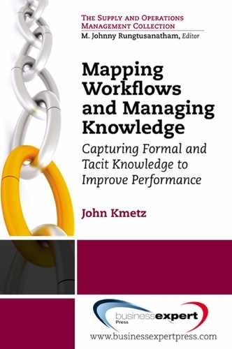
It may be helpful to think in terms of all possible outcomes of a workflow and how these can be categorized. Figure 6.1 is a WFMA map of a fairly typical quality control process in manufacturing, in which items are sampled from a production run and returned if they are within specifications. Items not “on spec” may be repairable, and if so they are repaired and re-inspected, and returned to the flow of finished goods (assuming they meet specification on re-inspection). Items not repairable are simply scrapped.
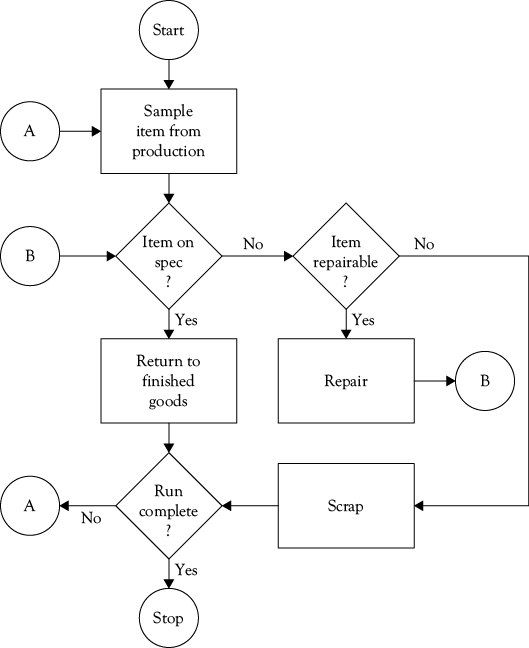
Figure 6.2 summarizes the outcomes of the workflow in Figure 6.1, in terms of the types discussed in Chapter 3, that is, normal or exception-handling outcomes, either of which can be a success or a failure. Regular production successes (which can be the output of successful innovation processes as well) are in the upper left cell of the figure. Successful exception-handling outcomes are directly beneath successful production in the lower left cell. In many cases, unsuccessful normal production may be an exception to be corrected, so it is possible that a successful exception-handling process may result in no loss to “regular” production, because those items return via the exception-handling process; it may also possible that an exception that costs more to correct than the value it adds will simply be discarded.
Failures can occur in either case, and these are shown in the right column of Figure 6.2 Undetected flaws (which might have been subject to correction had they been caught) are a residual of the quality control process that escape detection, and are sent into the environment (customers) to be detected there. Unsuccessful exception-handling processes result in “scrap” for the most part, regardless of what we call it.
Any of the outcomes in Figure 6.2 can be regarded as a “stock” in dynamic modeling terms, and the processes that create each of them a “flow,” where parts of some flows will probably overlap. If we have measures of most of the various outcomes, which is likely, then much of the basic information needed to construct a dynamic model is in hand. If not, we have at least identified processes that should be sampled and measured to provide the data we need—this will be discussed more fully below.
A number of microcomputer-based packages are available to support simulation by individuals. As noted earlier, one of the best of these is iThink, which develops its models based on diagrams of process variables created by the user. Part of my affection for iThink is because its underlying assumptions and conventions are highly compatible with my own, and transition from a WFMA static model to an iThink dynamic model is therefore greatly simplified. iThink opens to a mapping “scratchpad,” where users can rough out the model logic they would like to develop, and then go on to fully model and test it. All iThink math and program code are written in the background, although they can be seen and manipulated directly if desired. For most users, the graphical interface will more than suffice.
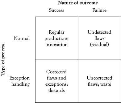
Figure 6.3 shows what the workflow map in Figure 6.1 looks like when translated into a dynamic model in iThink software. Raw materials are brought from their sources (represented as a “cloud” icon) through a flow, and become a “stock” of work in process. The flow of initial finished production is sampled for inspection, shown by the solid “action” arrow from initial production to inspection. Inspection uses a set of data and procedures, shown as a dashed “information” arrow to determine whether sampled items are within specifications or not—those within spec are returned to the flow of materials ready to ship to customers, and those not acceptable are rejects which are a loss of available inventory; the “Return” arrow indicates that production inspected and acceptable is returned to the flow available to customers, while the “Inventory loss” arrow signifies a reduction of available product for customers. (I leave as a thought exercise the repair-and-re-inspect loop in Figure 6.1) All of the possible outcomes in either Figure 6.1 or 6.2 can occur in the dynamic model shown in Figure 6.3, but the diagram in Figure 6.3 is quite unlike the WFMA maps we have been seeing in this book.
Some of the symbols used in Figure 6.3 are familiar WFMA friends with similar meanings—arrows showing movement, the decision diamond, the process block that represents a host of things. However, the circle is a “converter,” not a connector, and the connections between these symbols are governed by a strict set of programming rules, so that in many cases process logic cannot be represented as simply as with the static workflow mapping we have been using, because we are bound by the unseen programming rules that are in turn driven by the diagram above. Given the fact that these diagrams literally create a mathematical model of the process, these restrictions are not surprising. They mean, as mentioned above, that considerably more effort will be needed to create dynamic models than to create static workflow maps because the rules of iThink are more restrictive than WFMA. The same would be true of any simulation software, and many programs are much more complex than iThink.
This general approach of translating WFMA maps into dynamic models can be scaled down to the subprocesses within larger streams of activity, and can also be scaled up to apply to higher-level systems. Any such up- or down-scaling, however, depends on the information about processes available to the modeler; this is where WFMA becomes a necessary first step in system modeling. To dynamically model a process, a valid static model is a prerequisite, but a significant departure from creating static WFMA models is the need for process data.
Simulation Data Requirements
As a static model, WFMA can enable collection of data for analysis. Unlike static models, dynamic simulation requires prior definition of system states in terms of data and information which accurately reflects the inputs the system acquires and outputs the system produces. There are frequently many intermediate states of production and ancillary processes that may also need to be specified. To model any system, data will be required which can both inform the model on the properties of the inputs, and can generate representative final and intermediate outputs.
We are already familiar with two types of data, stocks and flows. For many WFMA analyses, we will be measuring these as incoming and outgoing inventory levels (whether in the form of manufactured parts, incoming and outgoing patients or students, documents processed or awaiting processing, or whatever it is that we do). For dynamic simulation, a third type of data will be needed, and that is the rate of movement of many of these items.
Rates are changes over some base value, usually expressed as a percentage or fraction. These can often be expressed as positive or negative values; “positive” and “negative” sometimes connote meanings other than mathematical, and for that reason I recommend description of rates in the most neutral language possible. We are all familiar with many kinds of rates, and use them in everyday discussion. In education we are interested in both the percentage of students who excel as well as the percentage who fail; in hospitals we are concerned with the rate of patient infection, expressed as a percentage or (hopefully) as the number on a larger base, perhaps the number of infections per thousand admissions; we measure speed as distance over time, and in most residential areas of the world the speed limit is 40 kilometers per hour (km/h) or 25 miles per hour (mph) in the United States.
Rates may be calculated from basic data measured on a workflow map. In Figure 6.1 we could measure the number of items sampled, the number on spec, the number not on spec but repairable, and so on for the entire workflow. We can also measure some rates directly, as total production over time (units per minute or hour or day, as appropriate). We can measure the time required to complete an inspection, and the length of time an item spends in the repair–re-inspect–return or discard subprocess. With a valid workflow map and measures taken from what is actually being done in the workflow, acquiring or creating meaningful rate information is greatly simplified, and confidence in the simulation models based on the data is enhanced.
This is not always the case, however. One of the frustrations that can afflict many modelers is that once a system workflow is mapped and understood, we may find there are neither metrics nor measurement processes that capture the data needed to model the system. In my Navy research, I was often astounded to find that information I assumed had been captured somewhere in the system had not. For example, in the early days of examining the performance of the VAST shops, I found that there had never been a requirement for benchmark “standard” times to be available for all of the avionics components serviced by the VAST tester. My interests in this information were several, not the least being able to get an idea of “how badly VAST was performing” against its intended capabilities, if it was the culprit in the maintenance workflow that so many believed it to be. Lacking that, I went looking for some average data on repair activity—I knew that the Navy collected the clock times for every AC that entered and left the repair process in the VAST shop when the item was serviced, and I thought surely someone had crunched the numbers to get some idea what the averages were. None ever had, so I thought certainly there must be some such information on the really difficult-to-repair ACs that so often seemed to jam up the system, but those didn’t exist, either. To complete my research on this part of the repair cycle, I had to take nearly a year to get the raw data from the Navy, hire a graduate assistant, and then extract what we needed from scratch.
This is not a phenomenon that applies only to the factory floor or the maintenance cycle. Recent interest in “evidence-based medicine,” in large part, is partly derived from belated recognition of the lack of output data possessed by the medical profession—in short, there are many drugs, and medical and surgical procedures, which produce highly variable final results. Only now is the profession beginning to take steps to measure and evaluate these outcomes, with a major objective being to validate procedures that until now have largely been taken on the faith that they are technically possible.7
In my own experience, this can be one of the more frustrating aspects of much dynamic modeling, and in some cases a cause for dynamic models to get a “bad rap.” Users will complain, often with good reason, that a model does a very poor job of representing a system, and generates outputs that are contrary to history and everyday experience. In the cases I have worked with, this has usually been attributable to poor understanding of the system in the first place, that is, that valid static models were not generated as a baseline for dynamic modeling, or in other instances, the modelers wanted to model the system that “should be,” only to learn that it produced many outputs that should not be.
Simulation as Simulation
Simulation is always caught between two opposing threats, one of excessive simplification and the other of excessive complexity. One of the advantages of simulation models is that they allow us to take complex real entities and reduce them to their essentials, to then determine how much of the system’s outcomes and behaviors are due to those essentials, among other questions. If one attempts to add all possible variables to account for every source of variability in the system, the model then becomes complex and unwieldy, and so difficult to understand that even if it did produce accurate results, it might still lack credibility. Many years of experience suggest that the relationship between model complexity and outcome credibility is an inverted “U” shape, with the best credibility in the midrange of model complexity.
Experience with different types of simulations has shown that there are positive and negative outcomes that obtain to modeling. There is no question that simulations are generally cheaper, safer, faster, and more controllable than manipulation of real-world systems; in fact, they are often the only way to acquire insights. The idea of the “long run” in decision making is untestable in the real world—there are many investment decisions that can only be made once, and if a negative outcome results, there is no future for a “long run” to happen. Simulations like Monte Carlo models, the use of Crystal Ball™ to simulate project outcomes, and dynamic simulations are the only environments in which multiple trials of a potential decision that plays out over a long period of time can be evaluated. In many cases, such models are the only possibility of “replicating” outcomes like scientific and economic experiments.
At the same time, there are negatives associated with simulation, some of which are direct consequences of the fact that we can do them. The fact that simulation is the only source of information on the “long run” may convince us that any simulation result is an accurate simulation result, in terms of the real world. We forget the ancient IT wisdom of “garbage in, garbage out,” and imbue simulation outputs with far more credibility than they deserve. The simplifications and assumptions necessary to build a model in the first place may be overlooked, and so what the computer does becomes “reality,” to the extent that disconfirming evidence from the real world is disregarded as incorrect when it disagrees with the results of the model. Such overconfidence in mathematical models was a major contributor to the meltdown of long-term capital management in 1998.
The discipline of economics illustrates many of the problems inherent in the model versus reality versions of the universe. Economics has struggled with a major challenge over the centuries, which is how to explain the behavior of masses of producers and consumers in terms of presumably rational decisions and actions based on self-interest. From a basis of observation and insight, modern economics has evolved into an exercise in mathematics and modeling, requiring enormous energy and effort to yield results that appear to be consistent with the real world (so long as the word “assume” is allowed liberal usage in those explanations—I remember attending economics seminars with U.S. colleagues in Bulgaria in the early 1990s, and at the end of one of these one of the audience members said to me, with great exasperation, “I thought you Americans really knew how an economy works, but now I think that all you know is how to make assumptions!”). The economic and financial global meltdown of 2008–2009 shook much of economics to its roots, not least the redoubtable Alan Greenspan, who admitted to being “shocked” at the extent to which cherished assumptions about the nature of markets had failed to hold up. At the end of the day, this is a case where the mental models of economists, made tangible through computers and software, faced head-on confrontations with the realities of market behavior, and many of them still have difficulty accepting the shortcomings of their models.
One of the principal confrontations at present is the debate between economists who adhere to the rational model of economics and those who argue that actual human behavior does not follow the assumed rules of rationality in that model; the latter group are appropriately termed “behavioral economists.” Behavioral economics (and its close relative, behavioral finance) contends that human decision making departs significantly from the narrow confines of pure self-interested rationality, and results in economic behavior that is often quite different from what traditional economics would predict. The mental model of the behavioral economists is very different from that of their rational-behavior colleagues, and it seems reasonable to expect that the contest between these schools of thought will be long and intense. The behavioralists point out that there is a long history of well-structured arguments to support their models. Recently, the recurring phenomenon of the economic “bubble” has become a focal point in this debate—in the mental models of many rationalists, there are no such things; in the models of the behavioralists, they are real and inevitable. For what it’s worth, my vote supports the behavioralists.
The point of all this is that there is no simple, surefire way to resolve the problem of whether to believe a model or not. If our basic mental models are incorrect from the outset, all we can do is model that incorrect belief system; even if it is correct, we will still be likely to face major challenges in constructing the model. One argument is that the ultimate issue is simply the confidence one has in a model, and three tests are proposed for building confidence.8 First, one can test the structure of the model—are the variables in the model, the relationships between them, and the dynamic linkages in it consistent with what we observe in the real world? Deviations matter. Second, is the behavior of the model consistent with the behavior of the real system? Do the parameters of the model produce results consistent with time series data from the system? Third, do we learn from the model—do we gain insights from the model that inform us about previously unseen or unappreciated characteristics of the real system?
Even with these caveats, there is evidence of growing global application of dynamic simulation as a tool for competitive advantage.9 For those not yet using dynamic simulation as an aid to decision-making, it is worth knowing that along with that growth in application has grown a global network of users and modelers interested in a huge variety of problems. One does not have to work alone or reinvent the wheel—quite the opposite. The Stella and iThink communities have grown to the point where global user groups and interest groups have formed, and regular training is available for new and experienced users.
Dynamic Modeling and KM
To end this chapter and bring the discussion in this book somewhat full circle, it is worth noting that dynamic simulation can be a valuable KM asset as well as a tool, in that simulation may greatly help us to know what we know. Our mental models of how our processes work, the effectiveness of our overall business model in different environments or situations, and many other questions of both micro- and macro-significance to the organization can be tested and evaluated. Dynamic simulation opens new doors to the application of what we have in our data and knowledge bases, and extends these in ways that simple search processes, however effective they are, can never do. My experience in the NAVAIR workflow analysis showed that dynamic simulation works best when both formal and tacit knowledge are included, challenging though that may be.
“Systems thinking,” the subject of Chapter 2 and the conceptual core of dynamic simulation, is a new form of knowledge and KM in and of itself. Systems thinking forces us to examine not only the content of a knowledge base but the relationships between key elements of that content. It forces us to think about the structure of the knowledge base in ways that go far beyond simply the cataloging and indexing of information, and that enables many possible new insights into the meaning of the content.
Of course, the output of such modeling and simulation becomes part of an expanded knowledge base on the organization. Models create a base of “experimental” outcomes that go beyond the simple extrapolation of trends or other visible changes in data. Fundamental to the Shewhart cycle discussed in Chapter 4 is the concept of experimentation with new ideas and possible solutions to problems. The simulation of valid processes can be an important part of this cycle, in that it allows us to test some ideas without intervention in the actual organization. But whether our experiments are simulations based on specific processes that might be improved or on large-scale, macro-level strategic issues, we create new knowledge of potential outcomes resulting from changes, and this is extends existing knowledge in ways that otherwise cannot be achieved.
In this way, organizational learning, one of the key objectives of systems dynamic modelers, becomes partially a function of how we use what we think we know, rather than just having a large knowledge base—again, this learning involves understanding of relationships instead of accounting for stocks and flows alone, and may take several forms.10 In Chapter 3 we briefly alluded to a “knowledge engineering” software project undertaken by Andersen Consulting.11 One of the major challenges of this project was to specify the “domain” in which such projects were being attempted. As the authors note:
There are a number of obstacles that hinder analysts when capturing domain knowledge. First, the domain information is increasingly distributed, as there are many stakeholders in a business system, including high-level managers, domain experts, users, system engineers and existing legacy documents about company policy, current processes and practices. This distribution and diversity makes the capture of knowledge very complex (and the different perspectives are necessary to provide a quality system). In addition, the knowledge of the domain experts is usually “hard-wired” in their internal memory structure, and difficult to bring to surface. The key domain experts tend also to be busy and unavailable. Building conceptual domain models is consequently, very difficult.
Despite our affection for the values and properties of “objective” decision making, there is much evidence that what humans do to make decisions frequently falls far from meeting the standards of being “objective.” Recent examples of decisions made by customers of Goldman Sachs, who essentially bought junk securities despite being characterized as “sophisticated investors” by Sachs, exemplify decision making on the basis of an unmeasurable intangible like “reputation.” In anticipation of “3G wireless,” European telecommunication service providers in the 1990s ran up a huge bubble for bandwidth to accommodate 3G services, despite the fact that the technology had not yet been invented nor had anyone a clear idea whether consumers would want what they might get with 3G.12 A decade later, AT&T got exclusive rights to distribute Apple’s iPhone in the United States on their network, only to find that the demand for bandwidth so far exceeded their capacity that they had to give away an application to track where telephone calls were being dropped, and consider surcharging those who used the very 3G services the iPhone was designed to provide! So confident were the Western Allies of the Nazi collapse in 1944 that they launched a disastrous attack into Holland that resulted in military failure at the cost of thousands of deaths, both military and civilian.13 When one pilot spotted two seasoned SS Panzer divisions hidden in a supposedly lightly defended area designated to be a drop zone for 8,000 Polish paratroopers, and showed his superiors photographs of their tanks and artillery, the pilot was asked, “Do you want to be the one to rock the boat?” The lists of these kinds of boondoggle decisions extends back at least to the tulip bubble,14 and before, and they all incorporate our ingrained human subjectivity in the processing of information.
Simulation may help resolve this kind of barrier to KM by evaluation of the mental models implicitly or explicitly held by these members of the organizational domain. The simulation study of the demise of the old Saturday Evening Post mentioned at the beginning of this chapter is an example of this kind of learning—what was discovered through simulation was that the mental models of the key variables and their impact on profitability, as held by domain stakeholders, were essentially deficient.15 They did not comprehend feedback relationships between the variables over the long term, and so made short-term decisions that ultimately defeated the system’s ability to stabilize in a profitable equilibrium. The “system,” in this case, included subscribes, advertisers, and distributors, all of whom had somewhat conflicting profit objectives in their relationship to the magazine’s management, but if enough time were given for changes in advertising rates, subscription rates, and the like to “work through the system,” all could have met an optimal level of financial return. These relationships were not intuitively obvious, did not work through the system on a schedule consistent with financial reporting cycles, and the simulation capability to examine the unintentionally destructive decisions management made did not exist to help managers at that time.
Figure 6.4 illustrates this in the context of the VAST shop problem we have heard of throughout this book. The mental model of the avionics workflow consisted of a simple FIFO model exactly like that used in many financial accounting applications. The control feedforward was to follow the FIFO rule; the feedback on effectiveness was on how well this worked. So long as the range of inquiry into the problems of keeping aircraft supplied with avionics was restricted to this question, no one could come up with an effective answer. Looking at avionics stocks and flows independently from this perspective shed little light on the reasons for lack of spare avionics once a cruise got underway with full air operations.
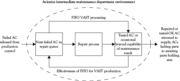
Organizations can learn to examine which of the many variables decision makers must manage to actually affect output. Not every input to a system is equally important in determining its output, and most are not. A model can test not only our mental model of what these variables are, but also the weights they have in producing outputs and adding value. Needless to say, once we understand the underlying structure of what we do to add value to our outputs, the better our chance of discovering new competitive advantage through alternative approaches. In the case of the avionics maintenance process, the key variables were information about the many activities comprising the repair cycle, and information about the current mission requirements; together, they enabled the managers of the repair process to select the correct ACs for repair in consideration of the overall status of avionics assets, which consisted of both the Supply “stocks” and the work-in-process “flows.” These had to be evaluated simultaneously and continuously since the status of both changed continuously and had to be reevaluated every time a new AC was inducted into the repair workflow. FIFO, in short, had no value in determining the next AC to select for repair.
In many respects, simulation is an important element of a true decision support system, arguably one of the first and most fundamental KM systems. The successful resolution of the problem of VAST production was actually a resolution of a much larger repair-cycle problem in which VAST was only one factor. When this was realized, simulation modeling was used to investigate the effect of changes in the scope of information used to manage the repair workflow. This revealed not only key variables to measure, but important and previously unrecognized relationships between them, and enabled creation of a decision support system for the VAST shop, the VAST automated management program; this, in turn, proved so effective that it became the basis for a decision support program for all naval aircraft maintenance, the automated production management module (APMM). APMM was both a simulation of the avionics maintenance system and a tool to manage it; it was part of the knowledge base for NAVAIR and a tool to manage that knowledge. It is now considered “legacy” software, but the system relationships that were embodied in it and were key to its effectiveness remain in place in the new generation of aircraft maintenance management to this day.
Summary
This short chapter has been intended to introduce readers to the concept of modeling and simulation as tools based on systems thinking. Its purpose is to make us aware of these as extensions of many of the fundamental ideas and methods we have learned in connection with basic WFMA, and which in a number of ways are also foundations of WFMA. Going to the next level of dynamic simulation is a discontinuous step from the deliberately simple steps in the Kmetz method of WFMA, but one well worth considering for the value it can add. Much of what might be learned from process understanding lies in teasing out the relationships between variables in a process, and WFMA is a major contributor to that knowledge, both formal and tacit; the dynamics and relationships over time are the next contributors, and simulation can open the door to these.